Random Search for Hyper-Parameter Optimization - Journal of ...
←
→
Page content transcription
If your browser does not render page correctly, please read the page content below
Journal of Machine Learning Research 13 (2012) 281-305                  Submitted 3/11; Revised 9/11; Published 2/12

                Random Search for Hyper-Parameter Optimization

James Bergstra                                                       JAMES . BERGSTRA @ UMONTREAL . CA
Yoshua Bengio                                                          YOSHUA . BENGIO @ UMONTREAL . CA
Département d’Informatique et de recherche opérationnelle
Université de Montréal
Montréal, QC, H3C 3J7, Canada

Editor: Leon Bottou

                                                         Abstract
     Grid search and manual search are the most widely used strategies for hyper-parameter optimiza-
     tion. This paper shows empirically and theoretically that randomly chosen trials are more efficient
     for hyper-parameter optimization than trials on a grid. Empirical evidence comes from a compar-
     ison with a large previous study that used grid search and manual search to configure neural net-
     works and deep belief networks. Compared with neural networks configured by a pure grid search,
     we find that random search over the same domain is able to find models that are as good or better
     within a small fraction of the computation time. Granting random search the same computational
     budget, random search finds better models by effectively searching a larger, less promising con-
     figuration space. Compared with deep belief networks configured by a thoughtful combination of
     manual search and grid search, purely random search over the same 32-dimensional configuration
     space found statistically equal performance on four of seven data sets, and superior performance
     on one of seven. A Gaussian process analysis of the function from hyper-parameters to validation
     set performance reveals that for most data sets only a few of the hyper-parameters really matter,
     but that different hyper-parameters are important on different data sets. This phenomenon makes
     grid search a poor choice for configuring algorithms for new data sets. Our analysis casts some
     light on why recent “High Throughput” methods achieve surprising success—they appear to search
     through a large number of hyper-parameters because most hyper-parameters do not matter much.
     We anticipate that growing interest in large hierarchical models will place an increasing burden on
     techniques for hyper-parameter optimization; this work shows that random search is a natural base-
     line against which to judge progress in the development of adaptive (sequential) hyper-parameter
     optimization algorithms.
     Keywords: global optimization, model selection, neural networks, deep learning, response surface
     modeling

1. Introduction

The ultimate objective of a typical learning algorithm A is to find a function f that minimizes some
expected loss L (x; f ) over i.i.d. samples x from a natural (grand truth) distribution Gx . A learning
algorithm A is a functional that maps a data set X (train) (a finite set of samples from Gx ) to a function
f . Very often a learning algorithm produces f through the optimization of a training criterion with
respect to a set of parameters θ. However, the learning algorithm itself often has bells and whistles
called hyper-parameters λ, and the actual learning algorithm is the one obtained after choosing
λ, which can be denoted Aλ , and f = Aλ (X (train) ) for a training set X (train) . For example, with a

c 2012 James Bergstra and Yoshua Bengio.
B ERGSTRA AND B ENGIO

Gaussian kernel SVM, one has to select a regularization penalty C for the training criterion (which
controls the margin) and the bandwidth σ of the Gaussian kernel, that is, λ = (C, σ).
    What we really need in practice is a way to choose λ so as to minimize generalization error
Ex∼Gx [L (x; Aλ (X (train) ))]. Note that the computation performed by A itself often involves an inner
optimization problem, which is usually iterative and approximate. The problem of identifying a
good value for hyper-parameters λ is called the problem of hyper-parameter optimization. This
paper takes a look at algorithms for this difficult outer-loop optimization problem, which is of great
practical importance in empirical machine learning work:

                                 λ(∗) = argmin Ex∼Gx [L x; Aλ (X (train) ) ].                       (1)
                                         λ∈Λ

In general, we do not have efficient algorithms for performing the optimization implied by Equa-
tion 1. Furthermore, we cannot even evaluate the expectation over the unknown natural distribution
Gx , the value we wish to optimize. Nevertheless, we must carry out this optimization as best we
can. With regards to the expectation over Gx , we will employ the widely used technique of cross-
validation to estimate it. Cross-validation is the technique of replacing the expectation with a mean
over a validation set X (valid) whose elements are drawn i.i.d x ∼ Gx . Cross-validation is unbiased
as long as X (valid) is independent of any data used by Aλ (see Bishop, 1995, pp. 32-33). We see in
Equations 2-4 the hyper-parameter optimization problem as it is addressed in practice:

                               λ(∗) ≈ argmin mean L x; Aλ (X (train) ) .                           (2)
                                        λ∈Λ      x∈X (valid)

                                  ≡ argmin Ψ(λ)                                                      (3)
                                        λ∈Λ

                                  ≈      argmin Ψ(λ) ≡ λ̂                                            (4)
                                      λ∈{λ(1) ...λ(S) }

     Equation 3 expresses the hyper-parameter optimization problem in terms of a hyper-parameter
response function, Ψ. Hyper-parameter optimization is the minimization of Ψ(λ) over λ ∈ Λ. This
function is sometimes called the response surface in the experiment design literature. Different data
sets, tasks, and learning algorithm families give rise to different sets Λ and functions Ψ. Knowing
in general very little about the response surface Ψ or the search space Λ, the dominant strategy for
finding a good λ is to choose some number (S) of trial points {λ(1) ...λ(S) }, to evaluate Ψ(λ) for each
one, and return the λ(i) that worked the best as λ̂. This strategy is made explicit by Equation 4.
     The critical step in hyper-parameter optimization is to choose the set of trials {λ(1) ...λ(S) }.
The most widely used strategy is a combination of grid search and manual search (e.g., LeCun
et al., 1998b; Larochelle et al., 2007; Hinton, 2010), as well as machine learning software packages
such as libsvm (Chang and Lin, 2001) and scikits.learn.1 If Λ is a set indexed by K configuration
variables (e.g., for neural networks it would be the learning rate, the number of hidden units, the
strength of weight regularization, etc.), then grid search requires that we choose a set of values for
each variable (L(1) ...L(K) ). In grid search the set of trials is formed by assembling every possible
combination of values, so the number of trials in a grid search is S = ∏Kk=1 |L(k) | elements. This
product over K sets makes grid search suffer from the curse of dimensionality because the number
of joint values grows exponentially with the number of hyper-parameters (Bellman, 1961). Manual
 1. scikits.learn: Machine Learning in Python can be found at http://scikit-learn.sourceforge.net.

                                                          282
R ANDOM S EARCH FOR H YPER -PARAMETER O PTIMIZATION
search is used to identify regions in Λ that are promising and to develop the intuition necessary to
choose the sets L(k) . A major drawback of manual search is the difficulty in reproducing results.
This is important both for the progress of scientific research in machine learning as well as for ease
of application of learning algorithms by non-expert users. On the other hand, grid search alone does
very poorly in practice (as discussed here). We propose random search as a substitute and baseline
that is both reasonably efficient (roughly equivalent to or better than combinining manual search
and grid search, in our experiments) and keeping the advantages of implementation simplicity and
reproducibility of pure grid search. Random search is actually more practical than grid search
because it can be applied even when using a cluster of computers that can fail, and allows the
experimenter to change the “resolution” on the fly: adding new trials to the set or ignoring failed
trials are both feasible because the trials are i.i.d., which is not the case for a grid search. Of course,
random search can probably be improved by automating what manual search does, i.e., a sequential
optimization, but this is left to future work.
There are several reasons why manual search and grid search prevail as the state of the art despite
decades of research into global optimization (e.g., Nelder and Mead, 1965; Kirkpatrick et al., 1983;
Powell, 1994; Weise, 2009) and the publishing of several hyper-parameter optimization algorithms
(e.g., Nareyek, 2003; Czogiel et al., 2005; Hutter, 2009):
• Manual optimization gives researchers some degree of insight into Ψ;
• There is no technical overhead or barrier to manual optimization;
• Grid search is simple to implement and parallelization is trivial;
• Grid search (with access to a compute cluster) typically finds a better λ̂ than purely manual
sequential optimization (in the same amount of time);
• Grid search is reliable in low dimensional spaces (e.g., 1-d, 2-d).
We will come back to the use of global optimization algorithms for hyper-parameter selection
in our discussion of future work (Section 6). In this paper, we focus on random search, that is, inde-
pendent draws from a uniform density from the same configuration space as would be spanned by a
regular grid, as an alternative strategy for producing a trial set {λ(1) ...λ(S) }. We show that random
search has all the practical advantages of grid search (conceptual simplicity, ease of implementation,
trivial parallelism) and trades a small reduction in efficiency in low-dimensional spaces for a large
improvement in efficiency in high-dimensional search spaces.
In this work we show that random search is more efficient than grid search in high-dimensional
spaces because functions Ψ of interest have a low effective dimensionality; essentially, Ψ of interest
are more sensitive to changes in some dimensions than others (Caflisch et al., 1997). In particular, if
a function f of two variables could be approximated by another function of one variable ( f (x1 , x2 ) ≈
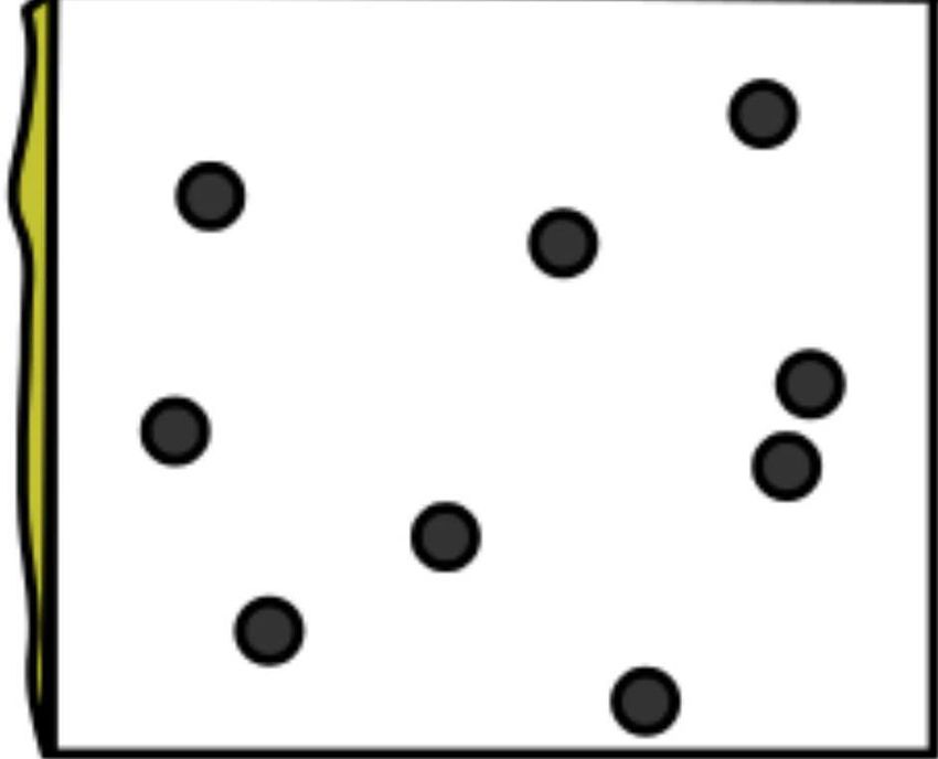
g(x1 )), we could say that f has a low effective dimension. Figure 1 illustrates how point grids
and uniformly random point sets differ in how they cope with low effective dimensionality, as in
the above example with f . A grid of points gives even coverage in the original 2-d space, but
projections onto either the x1 or x2 subspace produces an inefficient coverage of the subspace. In
contrast, random points are slightly less evenly distributed in the original space, but far more evenly
distributed in the subspaces.
If the researcher could know ahead of time which subspaces would be important, then he or she
could design an appropriate grid. However, we show the failings of this strategy in Section 2. For a
283B ERGSTRA AND B ENGIO
Grid Layout Random Layout
Unimportant parameter
Unimportant parameter
Important parameter Important parameter
Figure 1: Grid and random search of nine trials for optimizing a function f (x, y) = g(x) + h(y) ≈
g(x) with low effective dimensionality. Above each square g(x) is shown in green, and
left of each square h(y) is shown in yellow. With grid search, nine trials only test g(x)
in three distinct places. With random search, all nine trials explore distinct values of
g. This failure of grid search is the rule rather than the exception in high dimensional
hyper-parameter optimization.
given learning algorithm, looking at several relatively similar data sets (from different distributions)
reveals that on different data sets, different subspaces are important, and to different degrees. A grid
with sufficient granularity to optimizing hyper-parameters for all data sets must consequently be
inefficient for each individual data set because of the curse of dimensionality: the number of wasted
grid search trials is exponential in the number of search dimensions that turn out to be irrelevant for
a particular data set. In contrast, random search thrives on low effective dimensionality. Random
search has the same efficiency in the relevant subspace as if it had been used to search only the
relevant dimensions.
This paper is organized as follows. Section 2 looks at the efficiency of random search in practice
vs. grid search as a method for optimizing neural network hyper-parameters. We take the grid search
experiments of Larochelle et al. (2007) as a point of comparison, and repeat similar experiments
using random search. Section 3 uses Gaussian process regression (GPR) to analyze the results of
the neural network trials. The GPR lets us characterize what Ψ looks like for various data sets,
and establish an empirical link between the low effective dimensionality of Ψ and the efficiency
of random search. Section 4 compares random search and grid search with more sophisticated
point sets developed for Quasi Monte-Carlo numerical integration, and argues that in the regime of
interest for hyper-parameter selection grid search is inappropriate and more sophisticated methods
bring little advantage over random search. Section 5 compares random search with the expert-
guided manual sequential optimization employed in Larochelle et al. (2007) to optimize Deep Belief
Networks. Section 6 comments on the role of global optimization algorithms in future work. We
conclude in Section 7 that random search is generally superior to grid search for optimizing hyper-
parameters.
284R ANDOM S EARCH FOR H YPER -PARAMETER O PTIMIZATION
2. Random vs. Grid for Optimizing Neural Networks
In this section we take a second look at several of the experiments of Larochelle et al. (2007) us-
ing random search, to compare with the grid searches done in that work. We begin with a look
at hyper-parameter optimization in neural networks, and then move on to hyper-parameter opti-
mization in Deep Belief Networks (DBNs). To characterize the efficiency of random search, we
present two techniques in preliminary sections: Section 2.1 explains how we estimate the general-
ization performance of the best model from a set of candidates, taking into account our uncertainty
in which model is actually best; Section 2.2 explains the random experiment efficiency curve that
we use to characterize the performance of random search experiments. With these preliminaries
out of the way, Section 2.3 describes the data sets from Larochelle et al. (2007) that we use in our
work. Section 2.4 presents our results optimizing neural networks, and Section 5 presents our results
optimizing DBNs.
2.1 Estimating Generalization
Because of finite data sets, test error is not monotone in validation error, and depending on the set
of particular hyper-parameter values λ evaluated, the test error of the best-validation error configu-
ration may vary. When reporting performance of learning algorithms, it can be useful to take into
account the uncertainty due to the choice of hyper-parameters values. This section describes our
procedure for estimating test set accuracy, which takes into account any uncertainty in the choice
of which trial is actually the best-performing one. To explain this procedure, we must distinguish
between estimates of performance Ψ(valid) = Ψ and Ψ(test) based on the validation and test sets
respectively:
Ψ(valid) (λ) = meanx∈X (valid) L x; Aλ (X (train) ) ,
Ψ(test) (λ) = meanx∈X (test) L x; Aλ (X (train) ) .
Likewise, we must define the estimated variance V about these means on the validation and test sets,
for example, for the zero-one loss (Bernoulli variance):
Ψ(valid) (λ) 1 − Ψ(valid) (λ)
(valid)
V (λ) = , and
|X (valid) | − 1
Ψ(test) (λ) 1 − Ψ(test) (λ)
(test)
V (λ) = .
|X (test) | − 1
With other loss functions the estimator of variance will generally be different.
The standard practice for evaluating a model found by cross-validation is to report Ψ(test) (λ(s) )
for the λ(s) that minimizes Ψ(valid) (λ(s) ). However, when different trials have nearly optimal val-
idation means, then it is not clear which test score to report, and a slightly different choice of λ
could have yielded a different test error. To resolve the difficulty of choosing a winner, we report a
weighted average of all the test set scores, in which each one is weighted by the probability that its
particular λ(s) is in fact the best. In this view, the uncertainty arising from X (valid) being a finite sam-
ple of Gx makes the test-set score of the best model among λ(1) , ..., λ(S) a random variable, z. This
score z is modeled by a Gaussian mixture model whose S components have means µs = Ψ(test) (λ(s) ),
285B ERGSTRA AND B ENGIO
variances σ2s = V(test) (λ(s) ), and weights ws defined by
′
ws = P Z (s) < Z (s ) , ∀s′ 6= s , where
Z ∼N Ψ
(i) (valid) (i)
(λ ), V (valid) (i)
(λ ) .
To summarize, the performance z of the best model in an experiment of S trials has mean µz and
standard error σ2z ,
S
µz = ∑ ws µs , and (5)
s=1
S
σ2z = ∑ ws µ2s + σ2s − µ2z .
(6)
s=1
It is simple and practical to estimate weights ws by simulation. The procedure for doing so is to
repeatedly draw hypothetical validation scores Z (s) from Normal distributions whose means are the
Ψ(valid) (λ(s) ) and whose variances are the squared standard errors V(valid) (λ(s) ), and to count how
often each trial generates a winning score. Since the test scores of the best validation scores are
typically relatively close, ws need not be estimated very precisely and a few tens of hypothetical
draws suffice.
In expectation, this technique for estimating generalization gives a higher estimate than the
traditional technique of reporting the test set error of the best model in validation. The difference is
related to the variance Ψ(valid) and the density of validation set scores Ψ(λ(i) ) near the best value. To
the extent that Ψ(valid) casts doubt on which model was best, this technique averages the performance
of the best model together with the performance of models which were not the best. The next section
(Random Experiment Efficieny Curve) illustrates this phenomenon and discusses it in more detail.
2.2 Random Experiment Efficiency Curve
Figure 2 illustrates the results of a random experiment: an experiment of 256 trials training neural
networks to classify the rectangles data set. Since the trials of a random experiment are indepen-
dently identically distributed (i.i.d.), a random search experiment involving S i.i.d. trials can also
be interpreted as N independent experiments of s trials, as long as sN ≤ S. This interpretation al-
lows us to estimate statistics such as the minimum, maximum, median, and quantiles of any random
experiment of size s, where s is a divisor of S.
There are two general trends in random experiment efficiency curves, such as the one in Figure 2:
a sharp upward slope of the lower extremes as experiments grow, and a gentle downward slope of
the upper extremes. The sharp upward slope occurs because when we take the maximum over
larger subsets of the S trials, trials with poor performance are rarely the best within their subset. It
is natural that larger experiments find trials with better scores. The shape of this curve indicates
the frequency of good models under random search, and quantifies the relative volumes (in search
space) of the various levels of performance.
The gentle downward slope occurs because as we take the maximum over larger subsets of trials
(in Equation 6), we are less sure about which trial is actually the best. Large experiments average
together good validation trials with unusually high test scores with other good validation trials with
unusually low test scores to arrive at a more accurate estimate of generalization. For example,
286R ANDOM S EARCH FOR H YPER -PARAMETER O PTIMIZATION
rectangles images
0.80
0.75
0.70
accuracy
0.65
0.60
0.55
0.50
0.45
1 2 4 8 16 32 64 128
experiment size (# trials)
Figure 2: A random experiment efficiency curve. The trials of a random experiment are i.i.d, so
an experiment of many trials (here, 256 trials optimizing a neural network to classify the
rectangles basic data set, Section 2.3) can be interpreted as several independent smaller
experiments. For example, at horizontal axis position 8, we consider our 256 trials to
be 32 experiments of 8 trials each. The vertical axis shows the test accuracy of the best
trial(s) from experiments of a given size, as determined by Equation 5. When there are
sufficiently many experiments of a given size (i.e., 10), the distribution of performance
is illustrated by a box plot whose boxed section spans the lower and upper quartiles and
includes a line at the median. The whiskers above and below each boxed section show
the position of the most extreme data point within 1.5 times the inter-quartile range of the
nearest quartile. Data points beyond the whiskers are plotted with ’+’ symbols. When
there are not enough experiments to support a box plot, as occurs here for experiments of
32 trials or more, the best generalization score of each experiment is shown by a scatter
plot. The two thin black lines across the top of the figure mark the upper and lower
boundaries of a 95% confidence interval on the generalization of the best trial overall
(Equation 6).
consider what Figure 2 would look like if the experiment had included lucky trial whose validation
score were around 77% as usual, but whose test score were 80%. In the bar plot for trials of size
1, we would see the top performer scoring 80%. In larger experiments, we would average that 80%
performance together with other test set performances because 77% is not clearly the best validation
score; this averaging would make the upper envelope of the efficiency curve slope downward from
80% to a point very close to the current test set estimate of 76%.
Figure 2 characterizes the range of performance that is to be expected from experiments of vari-
ous sizes, which is valuable information to anyone trying to reproduce these results. For example, if
we try to repeat the experiment and our first four random trials fail to find a score better than 70%,
then the problem is likely not in hyper-parameter selection.
287B ERGSTRA AND B ENGIO
Figure 3: From top to bottom, samples from the mnist rotated, mnist background random, mnist
background images, mnist rotated background images data sets. In all data sets the
task is to identify the digit (0 - 9) and ignore the various distracting factors of variation.
2.3 Data Sets
Following the work of Larochelle et al. (2007) and Vincent et al. (2008), we use a variety of classi-
fication data sets that include many factors of variation.2
The mnist basic data set is a subset of the well-known MNIST handwritten digit data set (LeCun
et al., 1998a). This data set has 28x28 pixel grey-scale images of digits, each belonging to one of ten
classes. We chose a different train/test/validation splitting in order to have faster experiments and see
learning performance differences more clearly. We shuffled the original splits randomly, and used
10 000 training examples, 2000 validation examples, and 50 000 testing examples. These images
are presented as white (1.0-valued) foreground digits against a black (0.0-valued) background.
The mnist background images data set is a variation on mnist basic in which the white fore-
ground digit has been composited on top of a 28x28 natural image patch. Technically this was done
by taking the maximum of the original MNIST image and the patch. Natural image patches with
very low pixel variance were rejected. As with mnist basic there are 10 classes, 10 000 training
examples, 2000 validation examples, and 50 000 test examples.
The mnist background random data set is a similar variation on mnist basic in which the
white foreground digit has been composited on top of random uniform (0,1) pixel values. As with
mnist basic there are 10 classes, 10 000 training examples, 2000 validation examples, and 50 000
test examples.
The mnist rotated data set is a variation on mnist basic in which the images have been rotated
by an amount chosen randomly between 0 and 2π radians. This data set included 10000 training
examples, 2000 validation examples, 50 000 test examples.
2. Data sets can be found at http://www.iro.umontreal.ca/˜lisa/twiki/bin/view.cgi/Public/
DeepVsShallowComparisonICML2007.
288R ANDOM S EARCH FOR H YPER -PARAMETER O PTIMIZATION
Figure 4: Top: Samples from the rectangles data set. Middle: Samples from the rectangles images
data set. Bottom: Samples from the convex data set. In rectangles data sets, the image is
formed by overlaying a small rectangle on a background. The task is to label the small
rectangle as being either tall or wide. In convex, the task is to identify whether the set of
white pixels is convex (images 1 and 4) or not convex (images 2 and 3).
The mnist rotated background images data set is a variation on mnist rotated in which the
images have been rotated by an amount chosen randomly between 0 and 2π radians, and then sub-
sequently composited onto natural image patch backgrounds. This data set included 10000 training
examples, 2000 validation examples, 50 000 test examples.
The rectangles data set (Figure 4, top) is a simple synthetic data set of outlines of rectangles.
The images are 28x28, the outlines are white (1-valued) and the backgrounds are black (0-valued).
The height and width of the rectangles were sampled uniformly, but when their difference was
smaller than 3 pixels the samples were rejected. The top left corner of the rectangles was also
sampled uniformly, with the constraint that the whole rectangle fits in the image. Each image is
labelled as one of two classes: tall or wide. This task was easier than the MNIST digit classification,
so we only used 1000 training examples, and 200 validation examples, but we still used 50 000
testing examples.
The rectangles images data set (Figure 4, middle) is a variation on rectangles in which the
foreground rectangles were filled with one natural image patch, and composited on top of a different
background natural image patch. The process for sampling rectangle shapes was similar to the one
used for rectangles, except a) the area covered by the rectangles was constrained to be between
25% and 75% of the total image, b) the length and width of the rectangles were forced to be of at
least 10 pixels, and c) their difference was forced to be of at least 5 pixels. This task was harder
than rectangles, so we used 10000 training examples, 2000 validation examples, and 50 000 testing
examples.
The convex data set (Figure 4, bottom) is a binary image classification task. Each 28x28 image
consists entirely of 1-valued and 0-valued pixels. If the 1-valued pixels form a convex region in
image space, then the image is labelled as being convex, otherwise it is labelled as non-convex. The
convex sets consist of a single convex region with pixels of value 1.0. Candidate convex images
were constructed by taking the intersection of a number of half-planes whose location and orienta-
289B ERGSTRA AND B ENGIO
tion were chosen uniformly at random. The number of intersecting half-planes was also sampled
randomly according to a geometric distribution with parameter 0.195. A candidate convex image
was rejected if there were less than 19 pixels in the convex region. Candidate non-convex images
were constructed by taking the union of a random number of convex sets generated as above, but
with the number of half-planes sampled from a geometric distribution with parameter 0.07 and with
a minimum number of 10 pixels. The number of convex sets was sampled uniformly from 2 to
4. The candidate non-convex images were then tested by checking a convexity condition for every
pair of pixels in the non-convex set. Those sets that failed the convexity test were added to the data
set. The parameters for generating the convex and non-convex sets were balanced to ensure that the
conditional overall pixel mean is the same for both classes.
2.4 Case Study: Neural Networks
In Larochelle et al. (2007), the hyper-parameters of the neural network were optimized by search
over a grid of trials. We describe the hyper-parameter configuration space of our neural network
learning algorithm in terms of the distribution that we will use to randomly sample from that con-
figuration space. The first hyper-parameter in our configuration is the type of data preprocessing:
with equal probability, one of (a) none, (b) normalize (center each feature dimension and divide by
its standard deviation), or (c) PCA (after removing dimension-wise means, examples are projected
onto principle components of the data whose norms have been divided by their eigenvalues). Part
of PCA preprocessing is choosing how many components to keep. We choose a fraction of variance
to keep with a uniform distribution between 0.5 and 1.0. There have been several suggestions for
how the random weights of a neural network should be initialized (we will look at unsupervised
learning pretraining algorithms later in Section 5). We experimented with two distributions and two
scaling heuristics. The possible distributions were (a) uniform on (−1, 1), and (b) unit normal. The
two scaling heuristics were (a) a hyper-parameter multiplier between 0.1 and 10.0 divided by the
square root of the number of inputs (LeCun et al., 1998b), and (b) the square root of 6 divided by
the square root of the number of inputs plus hidden units (Bengio and Glorot, 2010). The weights
themselves were chosen using one of three random seeds to the Mersenne Twister pseudo-random
number generator. In the case of the first heuristic, we chose a multiplier uniformly from the range
(0.2, 2.0). The number of hidden units was drawn geometrically3 from 18 to 1024. We selected
either a sigmoidal or tanh nonlinearity with equal probability. The output weights from hidden units
to prediction units were initialized to zero. The cost function was the mean error over minibatches
of either 20 or 100 (with equal probability) examples at a time: in expectation these give the same
gradient directions, but with more or less variance. The optimization algorithm was stochastic gra-
dient descent with [initial] learning rate ε0 drawn geometrically from 0.001 to 10.0. We offered the
possibility of an annealed learning rate via a time point t0 drawn geometrically from 300 to 30000.
The effective learning rate εt after t minibatch iterations was
t0 ε0
εt = . (7)
max(t,t0 )
We permitted a minimum of 100 and a maximum of 1000 iterations over the training data, stopping
if ever, at iteration t, the best validation performance was observed before iteration t/2. With 50%
3. We will use the phrase drawn geometrically from A to B for 0 < A < B to mean drawing uniformly in the log domain
between log(A) and log(B), exponentiating to get a number between A and B, and then rounding to the nearest integer.
The phrase drawn exponentially means the same thing but without rounding.
290R ANDOM S EARCH FOR H YPER -PARAMETER O PTIMIZATION
probability, an ℓ2 regularization penalty was applied, whose strength was drawn exponentially from
3.1 × 10⁻⁷ to 3.1 × 10⁻⁵ . This sampling process covers roughly the same domain with the same
density as the grid used in Larochelle et al. (2007), except for the optional preprocessing steps. The
grid optimization of Larochelle et al. (2007) did not consider normalizing or keeping only leading
PCA dimensions of the inputs; we compare to random sampling with and without these restrictions.4
We formed experiments for each data set by drawing S = 256 trials from this distribution. The
results of these experiments are illustrated in Figures 5 and 6. Random sampling of trials is surpris-
ingly effective in these settings. Figure 5 shows that even among the fraction of jobs (71/256) that
used no preprocessing, the random search with 8 trials is better than the grid search employed in
Larochelle et al. (2007).
Typically, the extent of a grid search is determined by a computational budget. Figure 6 shows
what is possible if we use random search in a larger space that requires more trials to explore. The
larger search space includes the possibility of normalizing the input or applying PCA preprocessing.
In the larger space, 32 trials were necessary to consistently outperform grid search rather than 8,
indicating that there are many harmful ways to preprocess the data. However, when we allowed
larger experiments of 64 trials or more, random search found superior results to those found more
quickly within the more restricted search. This tradeoff between exploration and exploitation is
central to the design of an effective random search.
The efficiency curves in Figures 5 and 6 reveal that different data sets give rise to functions Ψ
with different shapes. The mnist basic results converge very rapidly toward what appears to be a
global maximum. The fact that experiments of just 4 or 8 trials often have the same maximum as
much larger experiments indicates that the region of Λ that gives rise to the best performance is
approximately a quarter or an eighth respectively of the entire configuration space. Assuming that
the random search has not missed a tiny region of significantly better performance, we can say that
random search has solved this problem in 4 or 8 guesses. It is hard to imagine any optimization
algorithm doing much better on a non-trivial 7-dimensional function. In contrast the mnist rotated
background images and convex curves show that even with 16 or 32 random trials, there is consid-
erable variation in the generalization of the reportedly best model. This indicates that the Ψ function
in these cases is more peaked, with small regions of good performance.
3. The Low Effective Dimension of Ψ
Section 2 showed that random sampling is more efficient than grid sampling for optimizing func-
tions Ψ corresponding to several neural network families and classification tasks. In this section
we show that indeed Ψ has a low effective dimension, which explains why randomly sampled trials
found better values. One simple way to characterize the shape of a high-dimensional function is
to look at how much it varies in each dimension. Gaussian process regression gives us the statis-
tical machinery to look at Ψ and measure its effective dimensionality (Neal, 1998; Rasmussen and
Williams, 2006).
We estimated the sensitivity of Ψ to each hyper-parameter by fitting a Gaussian process (GP)
with squared exponential kernels to predict Ψ(λ) from λ. The squared exponential kernel (or
Gaussian kernel) measures similarity between two real-valued hyper-parameter values a and b by
2
exp(− a−b l ). The positive-valued l governs the sensitivity of the GP to change in this hyper-
4. Source code for the simulations is available at https://github.com/jaberg/hyperopt.
291B ERGSTRA AND B ENGIO
mnist basic mnist background images mnist background random
1.0 1.0 1.0
0.9 0.9 0.9
0.8 0.8 0.8
accuracy
accuracy
accuracy
0.7 0.7 0.7
0.6 0.6 0.6
0.5 0.5 0.5
0.4 0.4 0.4
0.3 0.3 0.3
1 2 4 8 16 32 1 2 4 8 16 32 1 2 4 8 16 32
experiment size (# trials) experiment size (# trials) experiment size (# trials)
mnist rotated mnist rotated background images convex
1.0 1.0 1.0
0.9 0.9 0.9
0.8 0.8 0.8
accuracy
accuracy
accuracy
0.7 0.7 0.7
0.6 0.6 0.6
0.5 0.5 0.5
0.4 0.4 0.4
0.3 0.3 0.3
1 2 4 8 16 32 1 2 4 8 16 32 1 2 4 8 16 32
experiment size (# trials) experiment size (# trials) experiment size (# trials)
rectangles rectangles images
1.0 1.0
0.9 0.9
0.8 0.8
accuracy
accuracy
0.7 0.7
0.6 0.6
0.5 0.5
0.4 0.4
0.3 0.3
1 2 4 8 16 32 1 2 4 8 16 32
experiment size (# trials) experiment size (# trials)
Figure 5: Neural network performance without preprocessing. Random experiment efficiency
curves of a single-layer neural network for eight of the data sets used in Larochelle et al.
(2007), looking only at trials with no preprocessing (7 hyper-parameters to optimize).
The vertical axis is test-set accuracy of the best model by cross-validation, the horizontal
axis is the experiment size (the number of models compared in cross-validation). The
dashed blue line represents grid search accuracy for neural network models based on a
selection by grids averaging 100 trials (Larochelle et al., 2007). Random searches of 8
trials match or outperform grid searches of (on average) 100 trials.
parameter. The kernels defined for each hyper-parameter were combined by multiplication (joint
Gaussian kernel). We fit a GP to samples of Ψ by finding the length scale (l) for each hyper-
parameter that maximized the marginal likelihood. To ensure relevance could be compared between
hyper-parameters, we shifted and scaled each one to the unit interval. For hyper-parameters that
were drawn geometrically or exponentially (e.g., learning rate, number of hidden units), kernel
calculations were based on the logarithm of the effective value.
292R ANDOM S EARCH FOR H YPER -PARAMETER O PTIMIZATION
mnist basic mnist background images mnist background random
1.0 1.0 1.0
0.9 0.9 0.9
0.8 0.8 0.8
accuracy
accuracy
accuracy
0.7 0.7 0.7
0.6 0.6 0.6
0.5 0.5 0.5
0.4 0.4 0.4
0.3 0.3 0.3
1 2 4 8 16 32 64 1 2 4 8 16 32 64 1 2 4 8 16 32 64
experiment size (# trials) experiment size (# trials) experiment size (# trials)
mnist rotated mnist rotated background images convex
1.0 1.0 1.0
0.9 0.9 0.9
0.8 0.8 0.8
accuracy
accuracy
accuracy
0.7 0.7 0.7
0.6 0.6 0.6
0.5 0.5 0.5
0.4 0.4 0.4
0.3 0.3 0.3
1 2 4 8 16 32 64 1 2 4 8 16 32 64 1 2 4 8 16 32 64
experiment size (# trials) experiment size (# trials) experiment size (# trials)
rectangles rectangles images
1.0 1.0
0.9 0.9
0.8 0.8
accuracy
accuracy
0.7 0.7
0.6 0.6
0.5 0.5
0.4 0.4
0.3 0.3
1 2 4 8 16 32 64 1 2 4 8 16 32 64
experiment size (# trials) experiment size (# trials)
Figure 6: Neural network performance when standard preprocessing algorithms are considered (9
hyper-parameters). Dashed blue line represents grid search accuracy using (on average)
100 trials (Larochelle et al., 2007), in which no preprocessing was done. Often the extent
of a search is determined by a computational budget, and with random search 64 trials are
enough to find better models in a larger less promising space. Exploring just four PCA
variance levels by grid search would have required 5 times as many (average 500) trials
per data set.
Figure 7 shows the relevance of each component of Λ in modelling Ψ(λ). Finding the length
scales that maximize marginal likelihood is not a convex problem and many local minima exist. To
get a sense of what length scales were supported by the data, we fit each set of samples from Ψ
50 times, resampling different subsets of 80% of the observations every time, and reinitializing the
length scale estimates randomly between 0.1 and 2. Figure 7 reveals two important properties of Ψ
for neural networks that suggest why grid search performs so poorly relative to random experiments:
1. a small fraction of hyper-parameters matter for any one data set, but
293B ERGSTRA AND B ENGIO
mnist basic mnist background images mnist background random
h.u.
a.f.
w.a.
w.n.
w.p.
l.r.
l.a.
relevance (1 / length scale) relevance (1 / length scale) relevance (1 / length scale)
mnist rotated mnist rotated back. images convex
h.u.
a.f.
w.a.
w.n.
w.p.
l.r.
l.a.
relevance (1 / length scale) relevance (1 / length scale) relevance (1 / length scale)
Legend rectangles rectangles images
n. hidden units h.u.
activation . a.f.
initial W algo. w.a.
initial W norm w.n.
weight penalty w.p.
learning rate l.r.
learn rate anneal. l.a.
relevance (1 / length scale) relevance (1 / length scale)
Figure 7: Automatic Relevance Determination (ARD) applied to hyper-parameters of neural net-
work experiments (with raw preprocessing). For each data set, a small number of hyper-
parameters dominate performance, but the relative importance of each hyper-parameter
varies from each data set to the next. Section 2.4 describes the seven hyper-parameters in
each panel. Boxplots are obtained by randomizing the subset of data used to fit the length
scales, and randomizing the length scale initialization. (Best viewed in color.)
294R ANDOM S EARCH FOR H YPER -PARAMETER O PTIMIZATION
2. different hyper-parameters matter on different data sets.
Even in this simple 7-d problem, Ψ has a much lower effective dimension of between 1 and 4,
depending on the data set. It would be impossible to cover just these few dimensions with a reli-
able grid however, because different data sets call for grids on different dimensions. The learning
rate is always important, but sometimes the learning rate annealing rate was important (rectangles
images), sometimes the ℓ2 -penalty was important (convex, mnist rotated), sometimes the number
of hidden units was important (rectangles), and so on. While random search optimized these Ψ
functions with 8 to 16 trials, a grid with, say, four values in each of these axes would already require
256 trials, and yet provide no guarantee that Ψ for a new data set would be well optimized.
Figure 7 also allows us to establish a correlation between effective dimensionality and ease of
optimization. The data sets for which the effective dimensionality was lowest (1 or 2) were mnist
basic, mnist background images, mnist background random, and rectangles images. Looking
back at the corresponding efficiency curves (Figure 5) we find that these are also the data sets
whose curves plateau most sharply, indicating that these functions are the easiest to optimize. They
are often optimized reasonably well by just 2 random trials. Looking to Figure 7 at the data sets with
largest effective dimensionality (3 or 4), we identify convex, mnist rotated, rectangles. Looking
at their efficiency curves in Figure 5 reveals that they consistently required at least 8 random trials.
This correlation offers another piece of evidence that the effective dimensionality of Ψ is playing a
strong role in determining the difficulty of hyper-parameter optimization.
4. Grid Search and Sets with Low Effective Dimensionality
It is an interesting mathematical challenge to choose a set of trials for sampling functions of un-
known, but low effective dimensionality. We would like it to be true that no matter which dimen-
sions turn out to be important, our trials sample the important dimensions evenly. Sets of points with
this property are well studied in the literature of Quasi-Random methods for numerical integration,
where they are known as low-discrepancy sets because they try to match (minimize discrepancy
with) the uniform distribution. Although there are several formal definitions of low discrepancy,
they all capture the intuition that the points should be roughly equidistant from one another, in order
that there be no “clumps” or “holes” in the point set.
Several procedures for constructing low-discrepancy point sets in multiple dimensions also try
to ensure as much as possible that subspace projections remain low-discrepancy sets in the subspace.
For example, the Sobol (Antonov and Saleev, 1979), Halton (Halton, 1960), and Niederreiter (Brat-
ley et al., 1992) sequences, as well as latin hypercube sampling (McKay et al., 1979) are all more
or less deterministic schemes for getting point sets that are more representative of random uniform
draws than actual random uniform draws. In Quasi Monte-Carlo integration, such point sets are
shown to asymptotically minimize the variance of finite integrals faster than true random uniform
samples, but in this section, we will look at these point sets in the setting of relatively small sample
sizes, to see if they can be used for more efficient search than random draws.
Rather than repeat the very computationally expensive experiments conducted in Section 2,
we used an artificial simulation to compare the efficiency of grids, random draws, and the four
low-discrepancy point sets mentioned in the previous paragraph. The artificial search problem was
to find a uniformly randomly placed multi-dimensional target interval, which occupies 1% of the
volume of the unit hyper-cube. We looked at four variants of the search problem, in which the target
was
295B ERGSTRA AND B ENGIO
1. a cube in a 3-dimensional space,
2. a hyper-rectangle in a 3-dimensional space,
3. a hyper-cube in a 5-dimensional space,
4. a hyper-rectangle in a 5-dimensional space.
The shape of the target rectangle in variants (2) and (4) was determined by sampling side lengths
uniformly from the unit interval, and then scaling the rectangle to have a volume of 1%. This
process gave the rectangles a shape that was often wide or tall - much longer along some axes than
others. The position of the target was drawn uniformly among the positions totally inside the unit
hyper-cube. In the case of tall or wide targets (2) and (4), the indicator function [of the target] had
a lower effective dimension than the dimensionality of the overall space because the dimensions in
which the target is elongated can be almost ignored.
The simulation experiment began with the generation of 100 random search problems. Then for
each experiment design method (random, Sobol, latin hypercube, grid) we created experiments of
1, 2, 3, and so on up to 512 trials.5 The Sobol, Niederreiter, and Halton sequences yielded similar
results, so we used the Sobol sequence to represent the performance of these low-discepancy set
construction methods. There are many possible grid experiments of any size in multiple dimensions
(at least for non-prime experiment sizes). We did not test every possible grid, instead we tested
every grid with a monotonic resolution. For example, for experiments of size 16 in 5 dimensions
we tried the five grids with resolutions (1, 1, 1, 1, 16), (1, 1, 1, 2, 8), (1, 1, 2, 2, 4), (1, 1, 1, 4,
4), (1, 2, 2, 2, 2); for experiments of some prime size P in 3 dimensions we tried one grid with
resolution (1, 1, P). Since the target intervals were generated in such a way that rectangles identical
up to a permutation of side lengths have equal probability, grids with monotonic resolution are
representative of all grids. The score of an experiment design method for each experiment size was
the fraction of the 100 targets that it found.
To characterize the performance of random search, we used the analytic form of the expectation.
The expected probability of finding the target is 1.0 minus the probability of missing the target
with every single one of T trials in the experiment. If the volume of the target relative to the unit
hypercube is (v/V = 0.01) and there are T trials, then this probability of finding the target is
v T
1 − (1 − ) = 1 − 0.99T .
V
Figure 8 illustrates the efficiency of each kind of point set at finding the multidimensional in-
tervals. There were some grids that were best at finding cubes and hyper-cubes in 3-d and 5-d, but
most grids were the worst performers. No grid was competitive with the other methods at finding
the rectangular-shaped intervals, which had low effective dimension (cases 2 and 4; Figure 8, right
panels). Latin hypercubes, commonly used to initialize experiments in Bayesian optimization, were
no more efficient than the expected performance of random search. Interestingly, the Sobol se-
quence was consistently best by a few percentage points. The low-discrepancy property that makes
the Sobol useful in integration helps here, where it has the effect of minimizing the size of holes
where the target might pass undetected. The advantage of the Sobol sequence is most pronounced in
experiments of 100-300 trials, where there are sufficiently many trials for the structure in the Sobol
5. Samples from the Sobol sequence were provided by the GNU Scientific Library (M. Galassi et al., 2009).
296R ANDOM S EARCH FOR H YPER -PARAMETER O PTIMIZATION
Figure 8: The efficiency in simulation of low-discrepancy sequences relative to grid and pseudo-
random experiments. The simulation tested how reliably various experiment design meth-
ods locate a multidimensional interval occupying 1% of a unit hyper-cube. There is one
grey dot in each sub-plot for every grid of every experiment size that has at least two ticks
in each dimension. The black dots indicate near-perfect grids whose finest and coarsest
dimensional resolutions differ by either 0 or 1. Hyper-parameter search is most typi-
cally like the bottom-right scenario. Grid search experiments are inefficient for finding
axis-aligned elongated regions in high dimensions (i.e., bottom-right). Pseudo-random
samples are as efficient as latin hypercube samples, and slightly less efficient than the
Sobol sequence.
depart significantly from i.i.d points, but not sufficiently many trials for random search to succeed
with high probability.
A thought experiment gives some intuition for why grid search fails in the case of rectangles.
Long thin rectangles tend to intersect with several points if they intersect with any, reducing the
effective sample size of the search. If the rectangles had been rotated away from the axes used to
build the grid, then depending on the angle the efficiency of grid could approach the efficiency of
random or low-discrepancy trials. More generally, if the target manifold were not systematically
aligned with subsets of trial points, then grid search would be as efficient as the random and quasi-
random searches.
297B ERGSTRA AND B ENGIO
5. Random Search vs. Sequential Manual Optimization
To see how random search compares with a careful combination of grid search and hand-tuning
in the context of a model with many hyper-parameters, we performed experiments with the Deep
Belief Network (DBN) model (Hinton et al., 2006). A DBN is a multi-layer graphical model with
directed and undirected components. It is parameterized similarly to a multilayer neural network for
classification, and it has been argued that pretraining a multilayer neural network by unsupervised
learning as a DBN acts both to regularize the neural network toward better generalization, and to
ease the optimization associated with finetuning the neural network for a classification task (Erhan
et al., 2010).
A DBN classifier has many more hyper-parameters than a neural network. Firstly, there is the
number of units and the parameters of random initialization for each layer. Secondly, there are
hyper-parameters governing the unsupervised pretraining algorithm for each layer. Finally, there
are hyper-parameters governing the global finetuning of the whole model for classification. For the
details of how DBN models are trained (stacking restricted Boltzmann machines trained by con-
trastive divergence), the reader is referred to Larochelle et al. (2007), Hinton et al. (2006) or Bengio
(2009). We evaluated random search by training 1-layer, 2-layer and 3-layer DBNs, sampling from
the following distribution:
• We chose 1, 2, or 3 layers with equal probability.
• For each layer, we chose:
– a number of hidden units (log-uniformly between 128 and 4000),
– a weight initialization heuristic that followed from a distribution (uniform or normal),
a multiplier (uniformly between 0.2 and 2), a decision to divide by the fan-out (true or
false),
– a number of iterations of contrastive divergence to perform for pretraining (log-uniformly
from 1 to 10000),
– whether to treat the real-valued examples used for unsupervised pretraining as Bernoulli
means (from which to draw binary-valued training samples) or as a samples themselves
(even though they are not binary),
– an initial learning rate for contrastive divergence (log-uniformly between 0.0001 and
1.0),
– a time point at which to start annealing the contrastive divergence learning rate as in
Equation 7 (log-uniformly from 10 to 10 000).
• There was also the choice of how to preprocess the data. Either we used the raw pixels or
we removed some of the variance using a ZCA transform (in which examples are projected
onto principle components, and then multiplied by the transpose of the principle components
to place them back in the inputs space).
• If using ZCA preprocessing, we kept an amount of variance drawn uniformly from 0.5 to 1.0.
• We chose to seed our random number generator with one of 2, 3, or 4.
• We chose a learning rate for finetuning of the final classifier log-uniformly from 0.001 to 10.
298R ANDOM S EARCH FOR H YPER -PARAMETER O PTIMIZATION
• We chose an anneal start time for finetuning log-uniformly from 100 to 10000.
• We chose ℓ2 regularization of the weight matrices at each layer during finetuning to be either
0 (with probability 0.5), or log-uniformly from 10−7 to 10−4 .
This hyper-parameter space includes 8 global hyper-parameters and 8 hyper-parameters for each
layer, for a total of 32 hyper-parameters for 3-layer models.
A grid search is not practical for the 32-dimensional search problem of DBN model selection,
because even just 2 possible values for each of 32 hyper-parameters would yield more trials than
we could conduct (232 > 109 trials and each can take hours). For many of the hyper-parameters,
especially real valued ones, we would really like to try more than two values. The approach taken
in Larochelle et al. (2007) was a combination of manual search, multi-resolution grid search and
coordinate descent. The algorithm (including manual steps) is somewhat elaborate, but sensible,
and we believe that it is representative of how model search is typically done in several research
groups, if not the community at large. Larochelle et al. (2007) describe it as follows:
“The hyper-parameter search procedure we used alternates between fixing a neural net-
work architecture and searching for good optimization hyper-parameters similarly to
coordinate descent. More time would usually be spent on finding good optimization
parameters, given some empirical evidence that we found indicating that the choice of
the optimization hyper-parameters (mostly the learning rates) has much more influence
on the obtained performance than the size of the network. We used the same procedure
to find the hyper-parameters for DBN-1, which are the same as those of DBN-3 except
the second hidden layer and third hidden layer sizes. We also allowed ourselves to
test for much larger first-hidden layer sizes, in order to make the comparison between
DBN-1 and DBN-3 fairer.
“We usually started by testing a relatively small architecture (between 500 and 700
units in the first and second hidden layer, and between 1000 and 2000 hidden units
in the last layer). Given the results obtained on the validation set (compared to those
of NNet for instance) after selecting appropriate optimization parameters, we would
then consider growing the number of units in all layers simultaneously. The biggest
networks we eventually tested had up to 3000, 4000 and 6000 hidden units in the first,
second and third hidden layers respectively.
“As for the optimization hyper-parameters, we would proceed by first trying a few com-
binations of values for the stochastic gradient descent learning rate of the supervised
and unsupervised phases (usually between 0.1 and 0.0001). We then refine the choice of
tested values for these hyper-parameters. The first trials would simply give us a trend on
the validation set error for these parameters (is a change in the hyper-parameter making
things worse of better) and we would then consider that information in selecting ap-
propriate additional trials. One could choose to use learning rate adaptation techniques
(e.g., slowly decreasing the learning rate or using momentum) but we did not find these
techniques to be crucial.
There was large variation in the number of trials used in Larochelle et al. (2007) to optimize the
DBN-3. One data set (mnist background images) benefited from 102 trials, while another (mnist
background random) only 13 because a good result was found more quickly. The average number
299B ERGSTRA AND B ENGIO
mnist basic mnist background images mnist background random
mnist rotated mnist rotated back. images convex
accuracy
accuracy
experiment size (# trials) experiment size (# trials)
rectangles rectangles images
accuracy
accuracy
experiment size (# trials) experiment size (# trials)
Figure 9: Deep Belief Network (DBN) performance according to random search. Here random
search is used to explore up to 32 hyper-parameters. Results obtained by grid-assisted
manual search using an average of 41 trials are marked in finely-dashed green (1-layer
DBN) and coarsely-dashed red (3-layer DBN). Random experiments of 128 random trials
found an inferior best model for three data sets, a competitive model in four, and superior
model in one (convex). (Best viewed in color.)
of trials across data sets for the DBN-3 model was 41. In considering the number of trials per data
set, it is important to bear in mind that the experiments on different data sets were not performed
independently. Rather, later experiments benefited from the experience the authors had drawn from
earlier ones. Although grid search was part of the optimization loop, the manual intervention turns
the overall optimization process into something with more resemblance to an adaptive sequential
algorithm.
Random search versions of the DBN experiments from Larochelle et al. (2007) are shown in
Figure 9. In this more challenging optimization problem random search is still effective, but not
300You can also read