Stay at home policy is a case of exception fallacy: an internet based ecological study - Nature
←
→
Page content transcription
If your browser does not render page correctly, please read the page content below
www.nature.com/scientificreports
OPEN Stay‑at‑home policy
is a case of exception fallacy:
an internet‑based ecological study
R. F. Savaris1,4,5*, G. Pumi2, J. Dalzochio3 & R. Kunst3
A recent mathematical model has suggested that staying at home did not play a dominant role in
reducing COVID-19 transmission. The second wave of cases in Europe, in regions that were considered
as COVID-19 controlled, may raise some concerns. Our objective was to assess the association
between staying at home (%) and the reduction/increase in the number of deaths due to COVID-
19 in several regions in the world. In this ecological study, data from www.google.com/covid19/
mobility/, ourworldindata.org and covid.saude.gov.br were combined. Countries with > 100 deaths
and with a Healthcare Access and Quality Index of ≥ 67 were included. Data were preprocessed and
analyzed using the difference between number of deaths/million between 2 regions and the difference
between the percentage of staying at home. The analysis was performed using linear regression
with special attention to residual analysis. After preprocessing the data, 87 regions around the world
were included, yielding 3741 pairwise comparisons for linear regression analysis. Only 63 (1.6%)
comparisons were significant. With our results, we were not able to explain if COVID-19 mortality is
reduced by staying at home in ~ 98% of the comparisons after epidemiological weeks 9 to 34.
By late January, 2021, approximately 2.1 million people worldwide had died from the new coronavirus (COVID-
19)1. Wearing masks, taking personal precautions, testing for COVID-19 and social distancing have been advo-
cated for controlling the pandemic2–4. To achieve source control and stop transmission, social distancing has
been interpreted by many as staying at home. Such policies across multiple jurisdictions were suggested by some
experts5. These measures were supported by the World Health O rganization6,7, local a uthorities8–10, and encour-
aged on social media platforms11–13.
Some mathematical models and meta-analyses have shown a marked reduction in COVID-19 cases14–19 and
deaths20,21 associated with lockdown policies. Brazilian researchers have published mathematical models of
spreading patterns22 and suggested implementing social distancing measures and protection policies to control
virus transmission23. By May 5th, 2020, an early report, using the number of curfew days in 49 countries, found
evidence that lockdown could be used to suppress the spread of COVID-1924. Measures to address the COVID-19
pandemic with Non-Pharmacological Interventions (NPIs) were adopted after Brazil enacted Law No. 1 397925,
and this was followed by many states such as Rio de Janeiro26, the Federal District of Brasília (Decree No. 40520,
dated March 14th, 2020)27, the city of São Paulo (Decree No. 59.283, dated March 16th, 2020)28, and the State of
Rio Grande do Sul (Decree No. 55240/2020, dated May 10th, 2020)29. It was expected that, with these actions,
the number of deaths by COVID-19 would be reduced. Of note, the country’s most populous state, São Paulo,
adopted rigorous quarantine measures and put them into effect on March 24th, 2 02028. Internationally, Peru
adopted the world’s strictest l ockdown30.
Recently, Google LLC published datasets indicating changes in mobility (compared to an average baseline
before the COVID-19 pandemic). These reports were created with aggregated, anonymized sets of daily and
dynamic data at country and sub-regional levels drawn from users who had enabled the Location History setting
on their cell phones. These data reflect real-world changes in social behavior and provide information on mobility
trends for places like grocery stores, pharmacies, parks, public transit stations, retail and recreation locations,
1
School of Medicine, Department of Obstetrics and Gynecology, Universidade Federal do Rio Grande do Sul, Rua
Ramiro Barcelos 2400, Porto Alegre, RS CEP 90035‑003, Brazil. 2Mathematics and Statistics Institute and Programa
de Pós‑Graduação em Estatística, Universidade Federal do Rio Grande do Sul, 9500, Bento Gonçalves Avenue,
Porto Alegre, RS 91509‑900, Brazil. 3Applied Computing Graduate Program, University of Vale do Rio dos Sinos
(UNISINOS), Av. Unisinos, 950, São Leopoldo, RS 93022‑750, Brazil. 4Serv. Ginecologia e Obstetrícia, Hospital
de Clínicas de Porto Alegre, Rua Ramiro Barcelos 2350, Porto Alegre, RS CEP 90035‑903, Brazil. 5Postgraduate
of BigData, Data Science and Machine Learning Course, Unisinos, Porto Alegre, RS, Brazil. *email: rsavaris@
hcpa.edu.br
Scientific Reports | (2021) 11:5313 | https://doi.org/10.1038/s41598-021-84092-1 1
Vol.:(0123456789)www.nature.com/scientificreports/
residences, and workplaces, when compared to the baseline period prior to the pandemic31. Mobility in places
of residence provides information about the “time spent in residences”, which we will hereafter call “staying at
home” and use as a surrogate for measuring adherence to stay-at-home policies.
Studies using Google COVID-19 Community Mobility Reports and the daily number of new COVID-19
cases have shown that over 7 weeks a strong correlation between staying at home and the reduction of COVID-19
cases in 20 counties in the United S tates32; COVID-19 cases decreased by 49% after 2 weeks of staying at h ome33;
34
the incidence of new cases/100,000 people was also reduced ; social distancing policies were associated with
reduction in COVID-19 spread in the US35; as well as in 49 countries around the world24. A recent report using
Brazilian and European data has shown a correlation between NPI stringency and the spread of COVID-1936,37;
these analyses are debatable, however, due to their short time span and the type of time series b ehavior38, or for
35
their use of Pearson’s correlation in the context of non-stationary time series . The same statistical tools cannot
be applied to stationary and non-stationary time series a like39, and the latter is the case with this COVID-19
data. A 2020 Cochrane systematic review of this topic reported that they were not completely certain about this
evidence for several reasons. The COVID-19 studies based their models on limited data and made different
assumptions about the virus17; the stay-at-home variable was analyzed as a binary i ndicator40; and the number
of new cases could have been substantially undocumented41; all which may have biased the results. A sophis-
ticated mathematical model based on a high-dimensional system of partial differential equations to represent
disease spread has been p roposed42. According to this model, staying at home did not play a dominant role in
disease transmission, but the combination of these, together with the use of face masks, hand washing, early-
case detection (PCR test), and the use of hand sanitizers for at least 50 days could have reduced the number of
new cases. Finally, after 2 months, the simulations that drove the world to lockdown have been questioned43.
These studies applied relatively complex epidemiological models with unrealistic assumptions or parameters
that were either user-chosen or not deemed to work properly. Furthermore, the effects in the death rates were
directly inferred from the aftermath of a given intervention without a control group. Finally, the temporal delay
between the introduction of a certain intervention and the actual measurable variation in death rates was not
properly taken into account44,45.
The rationale we are looking for is the association between two variables: deaths/million and the percentage
of people who remained in their residences. Comparison, however, is difficult due to the non-stationary nature of
the data. To overcome these problems, we proposed a novel approach to assess the association between staying at
home values and the reduction/increase in the number of deaths due to COVID-19 in several regions around the
world. If the variation in the difference between the number of deaths/million in two countries, say A and B, and
the variation in the difference of the staying at home values between A and B present similar patterns, this is due
to an association between the two variables. In contrast, if these patterns are very different, this is evidence that
staying at home values and the number of deaths/million are not related (unless, of course, other unaccounted
for factors are at play). In view of this, the proposed approach avoids altogether the problems enumerated above,
allowing a new approach to the problem.
After more than 25 epidemiological weeks of this pandemic, verifying if staying at home had an impact on
mortality rates is of particular interest. A PUBMED search with the terms “COVID-19” AND (Mobility) (search
made on September 8th, 2020) yielded 246 articles; of these, 35 were relevant to mobility measures and COVID-
19, but none compared mobility reduction to mortality rates.
Results
A flowchart of the data manipulation is depicted in Fig. 1. Briefly, Google COVID-19 Community Mobility
Report data between February 16th and August 21st, 2020, yielded 138 separate countries and their regions.
The website Our World in Data provided data on 212 countries (between December 31st, 2019, and August
26th, 2020), and the Brazilian Health Ministry website provided data on all states (n = 27) and cities (n = 5,570)
in Brazil (February 25th to August 26th, 2020).
After data compilation, a total of 87 regions and countries were selected: 51 countries, 27 States in Brazil, six
major Brazilian State capitals [Manaus, Amazonas (AM), Fortaleza, Ceará (CE), Belo Horizonte, Minas Gerais
(MG), Rio de Janeiro, Rio de Janeiro (RJ), São Paulo, São Paulo (SP) and Porto Alegre, Rio Grande do Sul (RS)],
and three major cities throughout the world (Tokyo, Berlin and New York) (Fig. 1).
Characteristics of these 87 regions are presented in Table 1 (further details are in Supplemental Material—
Characteristics of Regions).
Comparisons. The restrictive analysis between controlled and not controlled areas yielded 33 appropriate
comparisons, as shown in Table 2. Only one comparison out of 33 (3%)—state of Roraima (Brazil) versus state
of Rondonia (Brazil)—was significant (p-value = 0.04). After correction for residual analysis, it did not pass the
autocorrelation test (Lagrange Multiplier test = 0.04). (Further details are in Supplemental Material—Restrictive
Analysis).
The global comparison yielded 3,741 combinations; from these, 184 (4.9%) had a p-value < 0.05, after cor-
recting for False Discovery Rate (Table S1). After performing the residual analysis, by testing for cointegration
between response and covariate, normality of the residuals, presence of residual autocorrelation, homoscedastic-
ity, and functional specification, only 63 (1.6%) of models passed all tests (Table S2). Closer inspection of several
cases where the model did not pass all the tests revealed a common factor: the presence of outliers, mostly due
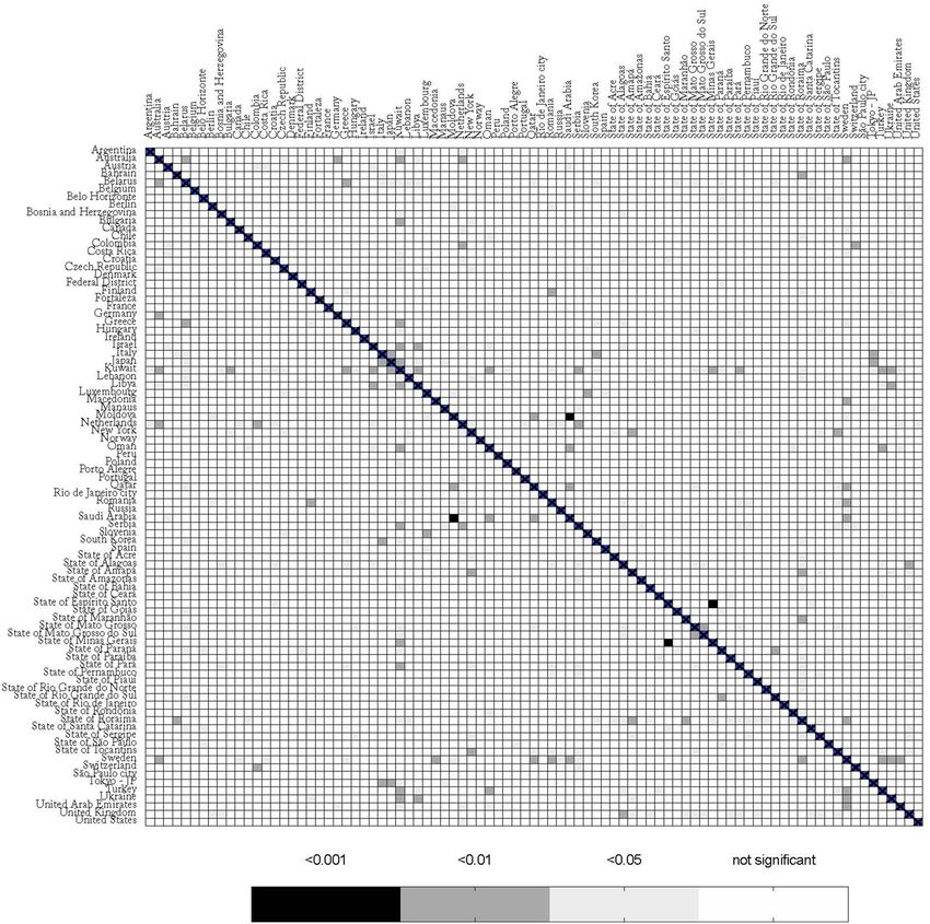
to differences in the epidemiological week in which deaths started to be reported. A heat map showing the com-
parison between the 87 regions is presented in Fig. 2.
Characteristics of these 87 regions are presented in Table 1 (further details are in Auxiliary Supplementary
Material—Characteristics of Regions) .
Scientific Reports | (2021) 11:5313 | https://doi.org/10.1038/s41598-021-84092-1 2
Vol:.(1234567890)www.nature.com/scientificreports/
Figure 1. Flow chart of the data setup (further details are in Auxiliary Supplementary Material—Flow chart).
Scientific Reports | (2021) 11:5313 | https://doi.org/10.1038/s41598-021-84092-1 3
Vol.:(0123456789)www.nature.com/scientificreports/
Region/Country Density people/km2 Urban Pop (%) HDI Population Land area ( km2)
Controlled areas
Austria 109 57 0.914 9,014,380 82,409
Bahrain 2,239 89 0.838 1,709,919 760
Belgium 383 98 0.919 11,597,489 30,280
Berlin 4,118 100 0.950 3,669,491 891
Canada 4 81 0.922 37,793,085 9,093,510
Czech Republic 139 74 0.891 10,712,102 78,866
Denmark 137 88 0.930 5,795,391 42,430
Finland 18 86 0.925 5,542,073 303,890
City of Fortaleza, Ceará, Brazil 7,786 100 0.754 2,686,612 312
France 119 82 0.891 65,296,176 547,557
Germany 240 76 0.939 83,825,861 348,560
Greece 81 85 0.870 10,414,904 128,900
Hungary 107 72 0.845 9,656,450 90,530
Ireland 72 63 0.942 4,946,213 68,890
Italy 206 69 0.883 60,447,728 294,140
Japan 347 92 0.915 126,414,795 364,555
Kuwait 240 100 0.808 4,280,111 17,820
Macedonia 83 59 0.759 2,083,360 25,220
City of Manaus, Amazonas, Brazil 158 100 0.737 2,219,580 11,401
Netherlands 508 92 0.934 17,140,821 33,720
New York City 10,194 100 0.941 8,336,817 784
Norway 15 83 0.954 5,427,784 365,268
Portugal 111 66 0.850 10,191,976 91,590
City of Rio de Janeiro, RJ, Brazil 5,266 100 0.799 6,747,815 1,200
Russia 9 74 0.824 145,944,331 16,376,870
Slovenia 103 55 0.902 2,078,983 20,140
South Korea 527 82 0.906 51,276,136 97,230
Spain 94 80 0.893 46,757,635 498,800
State of Acre 4 73 0.663 894,470 164,124
State of Amazonas 2 79 0.674 4,207,714 1,559,169
State of Pará 6 68 0.646 8,602,865 1,245,871
State of Roraima 2 76 0.707 631,181 223,645
Sweden 25 88 0.937 10,109,031 410,340
Switzerland 219 74 0.946 8,664,406 39,516
Tokyo, Japan 6,158 100 0.941 13,491,000 2,191
United Kingdom 279 83 0.920 67,886,011 241,930
Not controlled areas
Argentina 17 93 0.83 45,259,525 2,736,690
Australia 3 86 0.938 25,545,026 7,682,300
Belarus 47 79 0.817 9,448,832 202,910
City of Belo Horizonte, MG, Brazil 7167 100 0.81 2,521,564 331
Bosnia and Herzegovina 64 52 0.769 3,277,541 51,000
Bulgaria 64 76 0.861 6,940,012 108,560
Chile 26 85 0.847 19,141,470 743,532
Colombia 46 80 0.761 50,965,881 1,109,500
Costa Rica 100 80 0.794 5,101,269 51,060
Croatia 73 58 0.837 4,101,200 55,960
Brasília, FD Brazil 444.66 96.62 0.824 3,055,149 5,761
Israel 400 93 0.906 9,197,590 21,640
Lebanon 667 78 0.73 6,820,558 10,230
Libya 4 78 0.708 6,885,460 1,759,540
Luxembourg 242 88 0.909 627,509 2,590
Moldova 105 43 0.711 4,032,473 32,850
Oman 16 87 0.834 5,125,566 309,500
Peru 26 79 0.759 33,041,424 1,280,000
Continued
Scientific Reports | (2021) 11:5313 | https://doi.org/10.1038/s41598-021-84092-1 4
Vol:.(1234567890)www.nature.com/scientificreports/
Region/Country Density people/km2 Urban Pop (%) HDI Population Land area ( km2)
Poland 124 60 0.872 37,840,045 306,230
City of Porto Alegre, RS, Brazil 2837.53 100 0.805 1,488,252 495
Qatar 248 96 0.848 2,807,805 11,610
Romania 84 55 0.816 19,217,049 230,170
City of São Paulo, SP, Brazil 7398.26 100 0.805 12,325,232 1,521
Saudi Arabia 16 84 0.857 34,895,566 2,149,690
Serbia 100 56 0.799 8,731,751 87,460
State of Alagoas 112.23 73.64 0.631 3,351,543 27,843
State of Amapá 4.69 89.81 0.708 861,773 142,471
State of Bahia 24.82 72.07 0.66 14,930,634 564,760
State of Ceará 56.76 75.09 0.682 9,187,103 148,894
State of Espírito Santo 76.25 85.29 0.74 4,064,052 46,074
State of Goiás 17.65 90.29 0.735 7,113,540 340,203
State of Maranhão 19.81 63.07 0.639 7,114,598 329,642
State of Mato Grosso 3.36 81.9 0.725 3,526,220 903,207
State of Mato Grosso do Sul 6.86 85.64 0.729 2,809,394 357,146
State of Minas Gerais 33.41 83.38 0.731 21,292,666 586,521
State of Paraíba 66.7 75.37 0.658 4,039,277 56,467
State of Paraná 52.4 85.31 0.749 11,516,840 199,299
State of Pernambuco 89.63 80.15 0.673 9,616,621 98,068
State of Piauí 12.4 65.77 0.646 3,281,480 251,757
State of Rio de Janeiro 365.23 96.71 0.761 17,264,943 43,750
State of Rio Grande do Norte 59.99 77.82 0.684 3,534,165 52,810
State of Rio Grande do Sul 37.96 85.1 0.746 11,422,973 281,707
State of Rondônia 6.58 73.22 0.69 1,796,460 237,765
State of Santa Catarina 65.27 83.99 0.774 7,252,502 95,731
State of São Paulo 166.23 95.88 0.783 46,289,333 248,219
State of Sergipe 94.35 73.51 0.665 2,318,822 21,925
State of Tocantins 4.98 78.81 0.699 1,590,248 277,467
Turkey 110 76 0.807 84,477,895 769,630
Ukraine 75 69 0.75 43,691,576 579,320
United Arab Emirates 118 86 0.866 9,908,607 83,600
United States of America 36 82 0.92 331,303,997 9,834,000
Table 1. Characteristics of the 87 regions and countries used for comparison in the study. HDI = Human
Development Index (the higher, the better).
Comparisons. The restrictive analysis between controlled and not controlled areas yielded 33 appropriate com-
parisons, as shown in Table 2. Only one comparison out of 33 (3%)—State of Roraima (Brazil) versus State of
Rondonia (Brazil)—was significant (p-value = 0.04). After correction for residual analysis, it did not pass the
autocorrelation test (p-value of the Lagrange Multiplier test = 0.04). (Further details are in Auxiliary Supplemen-
tary Material—Restrictive Analysis).
The global comparison yielded 3,741 combinations; from these, 184 (4.9%) had a p-value < 0.05, after correct-
ing for False Discovery Rate (Table S1 suppl). After performing the residual analysis, by testing for cointegration
between response and covariate, normality of the residuals, presence of residual autocorrelation, homoscedastic-
ity, and functional specification, only 63 (1.6%) of models passed all tests (Table S2—suppl). Closer inspection of
several cases where the model did not pass all the tests revealed a common factor: the presence of outliers, mostly
due to differences in the epidemiological week in which deaths started to be reported. A heat map showing the
comparison between the 87 regions is presented in Fig. 2.
Discussion
We were not able to explain the variation of deaths/million in different regions in the world by social isolation,
herein analyzed as differences in staying at home, compared to baseline. In the restrictive and global comparisons,
only 3% and 1.6% of the comparisons were significantly different, respectively. These findings are in accordance
with those found by Klein et al.46 These authors explain why lockdown was the least probable cause for Sweden’s
high death rate from COVID-1946. Likewise, Chaudry et al. made a country-level exploratory analysis, using a
variety of socioeconomic and health-related characteristics, similar to what we have done here, and reported that
full lockdowns and wide-spread testing were not associated with COVID-19 mortality per million p eople47. Dif-
ferent from Chaudry et al., in our dataset, after 25 epidemiological weeks, (counting from the 9th epidemiological
Scientific Reports | (2021) 11:5313 | https://doi.org/10.1038/s41598-021-84092-1 5
Vol.:(0123456789)www.nature.com/scientificreports/
Region/country (controlled) Region/country (not controlled) Comparability p Value*
Austria Serbia 4–4 0.055
Bahrain City of Porto Alegre, RS, Brazil 4–4 0.911
Belgium Israel 4–4 0.114
Canada Australia 4–4 0.965
Czech Republic State of Alagoas 3–4 0.3501
Denmark Turkey 3–4 0.911
Finland State of Goiás 4–4 0.268
City of Fortaleza, CE, Brazil City of Belo Horizonte, MG, Brazil 4–4 0.301
France Ukraine 3–4 0.623
Germany Qatar 3–4 0.892
Greece Bulgaria 4–4 0.275
Ireland Croatia 4–4 0.711
Italy State of São Paulo 3–4 0.928
Japan Israel 3–4 0.102
Kuwait Luxembourg 3–4 0.060
City of Manaus, AM, Brazil Qatar 3–4 0.524
Macedonia Romania 3–4 0.6169
Netherlands City of Brasília, Brazil 3–4 0.459
New York City City of São Paulo, SP, Brazil 3–4 0.645
Norway Saudi Arabia 3–4 0.379
Portugal United Arab Emirates 3–4 0.248
Russia United States of America 3–4 0.557
Slovenia Poland 4–4 0.875
South Korea Lebanon 3–4 0.645
Spain State of Minas Gerais 3–4 0.853
State of Acre State of Amapá 4–4 0.803
State of Amazonas Colombia 3–4 0.638
State of Pará Libya 3–4 0.681
State of Roraima State of Rondônia 3–4 0.042
Sweden State of Bahia 4–4 0.131
Switzerland State of Espírito Santo 3–4 0.745
Tokyo, Japan City of São Paulo, SP, Brazil 4–4 0.731
United Kingdom State of Rio Grande do Sul 3–4 0.084
Table 2. Comparisons using the 4-point criteria. Comparability was considered if at least 3 out of 4 of the
following conditions were similar: a) population density, b) percentage of the urban population, c) Human
Development Index and d) total area of the region. Similarity was considered adequate when a variation in
conditions a), b) and c) was within 30%, while, for condition d), a variation of 50% was considered adequate
(Further details are in Auxiliary Supplementary Material—4 point criteria). *Linear regression.
week onwards in 2020) we included regions and countries with a "plateau" and a downslope phase in their
epidemiological curves. Our findings are in accordance with the dataset of daily confirmed COVID-19 deaths/
million in the UK. Pubs, restaurants, and barbershops were open in Ireland on June 29th and masks were not
mandatory48; after more than 2 months, no spike was observed; indeed, death rates kept falling49. Peru has been
considered to be the most strict lockdown country in the w orld30, nevertheless, by September 20th, it had the
highest number of deaths/million50. Of note, differences were also observed between regions that were considered
to be COVID-19 controlled, e.g., Sweden versus Macedonia. Possible explanations for these significant differences
may be related to the magnitude of deaths in these countries. After October 2020, when our study was published
in a preprint server for Health Sciences, new articles were published with similar r esults51–54.
Our results are different from those published by Flaxman et al. The authors applied a very complex calcula-
tion that NPIs would prevent 3.1 million deaths across 11 European c ountries44. The discrepant results can be
explained by different approaches to the data. While Flaxman et al. assumed a constant reproduction number
(Rt) to calculate the total number of deaths, which eventually did not occur, we calculated the difference between
the actual number of deaths between 2 countries/regions. The projections published by Flaxman et al.44 have
been disputed by other authors. Kuhbandner and Homburg described the circular logic that this study involved.
Flaxman et al. estimated the Rt from daily deaths associated with SARS-CoV-2 using an a priori restriction that Rt
may only change on those dates when interventions become effective. However, in the case of a finite population,
the effective reproduction number falls automatically and necessarily over time since the number of infections
would otherwise d iverge55. A recent preprint report from Chin et al.56 explored the two models proposed by
the Imperial College44 by expanding the scope to 14 European countries from the 11 countries studied in the
Scientific Reports | (2021) 11:5313 | https://doi.org/10.1038/s41598-021-84092-1 6
Vol:.(1234567890)www.nature.com/scientificreports/
Figure 2. Heat map comparing different regions with COVID-19. The bar below represents p-values for the
linear regression.
original paper. They added a third model that considered banning public events as the only covariate. The authors
concluded that the claimed benefits of lockdown appear grossly exaggerated since inferences drawn from effects
of NPIs are non-robust and highly sensitive to model s pecification56.
The same explanation for the discrepancy can be applied to other publications where mathematical models
were created to predict o utcomes14–18. Most of these studies dealt with COVID-19 cases 33,34 and not observed
deaths. Despite its limitations, reported deaths are likely to be more reliable than new case data. Further explana-
tions for different results in the literature, besides methodological aspects, could be justified by the complexity of
the virus dynamic, by its interaction with the environment, or they may be related to a seasonal pattern that was,
by coincidence, established at the same time when infection rates started to decrease due to seasonal d ynamics57.
It is unwise to try to explain a complex and multifactorial condition, with the inherent constant changes, using
a single variable. An initial approach would employ a linear regression to verify the influence of one factor over
an outcome. Herein we were not able to identify this association. Our study was not designed to explain why the
stay-at-home measures do not contain the spread of the virus SARS-CoV-2. However, possible explanations that
need further analysis may involve genetic f actors58, the increment of viral load, and transmission in households
and in close quarters where ventilation is reduced.
This study has a few limitations. Different from the established paradigm of randomized clinical trial, this is
an ecological study. An ecological study observes findings at the population level and generates hypotheses59.
Population-level studies play an essential part in defining the most important public health problems to be
tackled59, which is the case here. Another limitation was the use of Google Community Mobility Reports as a
surrogate marker for staying at home. This may underestimate the real value: for instance, if a user´s cell phone
is switched off while at home, the observation will be absent from the database. Furthermore, the sample does
not represent 100% of the population. This tool, nevertheless, has been used by other authors to demonstrate
the efficacy in reducing the number of new cases after N PI60,61. Using different methodologies for measuring
mobility may introduce bias and would prevent comparisons between different countries. The number of deaths
may be another issue. Death figures may be underestimated, however, reported deaths may be more relevant than
new case data. The arbitrary criteria used for including countries and regions, the restrictive comparisons, and
our definition of an area as COVID-19 controlled are open for criticism. Nonetheless, these arbitrary criteria
were created a priori to the selection of the countries. With these criteria, we expected to obtain representative
regions of the world, compare similar regions, and obtain accurate data. By using a HAQI of ≥ 67, we assumed
Scientific Reports | (2021) 11:5313 | https://doi.org/10.1038/s41598-021-84092-1 7
Vol.:(0123456789)www.nature.com/scientificreports/
that data from these countries would be accurate, reliable, and health conditions were generally good. Neverthe-
less, the global analysis of the regions (n = 3741 comparisons) overcame any issue of the restrictive comparison.
Indeed, the global comparison confirmed the results found in the restrictive one; only 1.6% of the death rates
could be explained by staying at home. Also, our effective sample size in all studies is only 25 epidemiological
weeks, which is a very small sample size for a time series regression. The small sample size and the non-stationary
nature of COVID-19 data are challenges for statistical models, but our analysis, with 25 epidemiological weeks,
is relatively larger than previous publications which used only 7 weeks62. A short interval of observation between
the introduction of an NPI and the observed effect on death rates yields no sound conclusion, and is a case
where the follow-up period is not long enough to capture the outcome, as seen in previous publications44,45. The
effects of small samples in this case are related to possible large type II errors and also affect the consistency of
the ordinary least square estimates. Nevertheless, given the importance of social isolation promoted by world
authorities63, we expected a higher incidence of significant comparisons, even though it could be an ecological
fallacy. The low number of significant associations between regions for mortality rate and the percentage of stay-
ing at home may be a case of exception fallacy, which is a generalization of individual characteristics applied at
the group-level characteristics64.
There are strengths to highlight. Inclusion criteria and the Healthcare Access and Quality Index were incor-
porated. We obtained representative regions throughout the world, including major cities from 4 different con-
tinents. Special attention was given to compiling and analyzing the dataset. We also devised a tailored approach
to deal with challenges presented by the data. To our knowledge, our modeling approach is unique in pooling
information from multiple countries all at once using up-to-date data. Some criteria, such as population density,
percentage of urban population, HDI, and HAQI, were established to compare similar regions. Finally, we gave
special attention to the residual analysis in the linear regression, an absolutely essential aspect of studies using
small samples.
In conclusion, using this methodology and current data, in ~ 98% of the comparisons using 87 different
regions of the world we found no evidence that the number of deaths/million is reduced by staying at home.
Regional differences in treatment methods and the natural course of the virus may also be major factors in this
pandemic, and further studies are necessary to better understand it.
Methods
Rationale and approach for analyzing the time series data. The proposed approach was tailored to
present a way to evaluate the influence of time spent at home and the number of deaths between two countries/
regions while avoiding common problems of other models presented in the literature. We focused on detect-
ing the variation of the differences between the number of deaths and how much people followed stay-at-home
orders in two regions in each epidemiological week.
For instance, let us consider two similar regions we shall call ‘Stay In county’ and ‘Go Out county’. Both
regions started with the same number of cases. After the first 1000 cases were recorded, Stay In county declared
that all people should stay at home, while Go Out county allowed people to circulate freely. After a few epide-
miological weeks, we examine the data collected on the number of deaths in both counties and how much time
people stayed at home by using geolocation software. If the difference between the number of deaths in Stay
In county and Go Out county (variable A) is affected by the difference of the percentage of time people stayed
at home in these two areas (variable B), then we can consider that the difference in the number of deaths by
COVID-19 is influenced by the difference in the percentage of time people stayed at home. Both effects can be
detected using linear regression and careful examination of the problem.
Time series on COVID-19 mortality (deaths/millions) display a non-stationary pattern. The daily data present
a very distinct seasonal behavior on the weekends, with valleys on Saturdays and Sundays followed by peaks on
Mondays (Figure S1). To account for seasonality, one may introduce dummy variables for Saturdays, Sundays,
and Mondays, regress the number of deaths in these dummy variables, and then analyze the residuals. How-
ever, in most cases, the residuals are still non-stationary, and special treatment would be required in each case.
Although this approach may be feasible for a few series, we are interested in analyzing hundreds of time series
from different countries and regions. Hence, we need a more efficient way to deal with this amount of data. The
covariates present another issue in regressing the daily time series of deaths/staying at home. The covariates are
typically correlated with error terms due to public policies adopted by regions/countries. Mechanisms control-
ling social isolation are intrinsically related to the number of deaths/cases in each location. An increase in the
death rate may cause more stringent policies to be adopted, which increases the percentage of people staying
at home. This change causes an imbalance between the observed number of deaths and staying at home levels.
In a regression model, this discrepancy is accounted for in the error term. Hence, the error term will change in
accordance with staying at home levels.
Data aggregation by epidemiological week is a plausible alternative (Figure S2). In this way, artificial seasonal-
ity, imposed by work scheduled during weekends and the effect of governmental control over social interaction,
in a regression framework, are mitigated. The drawback is that the sample size is significantly reduced from
187 days (Figure S1) to 26 epidemiological weeks (Figure S2).
Aggregation by epidemiological week, however, still yields non-stationary time series in most cases. To
overcome this problem, we differentiated each time series. Recall that if Ztdenotes the number of deaths in the
t-th epidemiological week, we define the first difference of Zt as
Zt = Zt − Zt−1
Intuitively, Zt denotes the variation of deaths between weeks t and t-1, also known as the flux of deaths.
The same is valid for the staying at home time series. This simple operation yielded, in most cases, stationary
Scientific Reports | (2021) 11:5313 | https://doi.org/10.1038/s41598-021-84092-1 8
Vol:.(1234567890)www.nature.com/scientificreports/
time series, verified with the so-called Phillips-Perron stationarity t est65. In the few cases where the resulting
time series did not reject the null hypothesis of non-stationarity (technically, the existence of a unitary root, in
the time series characteristic polynomial), this was due to the presence of one or two outliers combined with the
small sample size. These outliers were usually related to the very low incidence of COVID-19 deaths by the 9th
epidemiological week when paired with countries with a significant number of deaths in that same week, thus
resulting in an outlier which cannot be accounted for by linear regression.
To investigate pairwise behavior, we propose a method to assess the relationship between deaths and stay-
ing at home data between various countries and regions. For two countries/regions, say A and B, let YtA and YtB
denote the number of deaths per million at epidemiological week t for country A and B respectively, while XtA
and XtB denote the staying at home at epidemiological week t for
A and B,
respectively. The idea is to regress the
difference YtA − YtB = YtA − YtB on XtA − XtB = XtA − XtB . Formally, we perform the regression
� YtA − YtB = β0 + β1 � XtA − XtB + εt ,
where β0 and β1 are unknown coefficients and εt denotes an error term. Estimation of β0 and β1 is carried out
through ordinary least squares. The interpretation of the model is important. We are regressing the difference in
the variation of deaths between locations A and B into the difference in the variation of staying at home values
between the same location.
If the number of deaths in locations
A and B have a similar functional behavior over time, then
Yt − Yt
tends
A B
to be near-constant, and YtA − YtB tends to oscillate around zero. If the same applies to XtA − XtB , then
we expect β1 = 0; consequently, we conclude that the behavior, between A and B, is similar and the number of
deaths and the percentage of staying at home are associated in these regions. The other non-spurious situation
implying β1 = 0 occurs when the variation in the number of deaths in locations A and B increases/decreases over
time following a certain pattern, while the variation in the percentage of “staying at home” values also increases/
decreases following the same pattern (apart from the direction). In this situation, we found different epidemio-
logical patterns as in the variation in the number of deaths, and in the staying at home values, in locations A and
B were on opposite trends. However, if these patterns were similar (proportional), this would be captured in the
difference and, as a consequence, in the regression. This means that the different trends were near proportional
and, hence, the variation in staying at home is associated with the variation in deaths.
In the section below “Definition of areas with and without controlled cases of COVID-19”, each country/
region was classified into a binary class: either controlled or not controlled areas for COVID-19. The proposed
method allows for insights regarding the association of the number of deaths and staying at home levels between
countries/regions with similar/different degrees of COVID-19 control. Assumptions related to consistency, effi-
ciency, and asymptotic normality of the ordinary least squares, in the context of time series regression, can
be found in66. Since we are comparing many time series, to avoid any problem with spurious regression, we
performed a cointegration test between the response and covariates. In this context, this is equivalent to test-
ing the stationarity of εt , which was done by performing the Phillips-Perron test. Residual analysis is of utmost
importance in linear regression, especially in the context of small samples. The steps and tests performed in the
residual analysis are described in the statistical analysis section.
Study design. This is an ecological study using data available on the Internet.
Setting—data collection on mobility. Google COVID-19 Community Mobility R eports31 provided
data on mobility from 138 countries67,68 and regions between February 15th and August 21st, 2020. Data regard-
ing the average times spent at home was generated in comparison to the baseline. Baseline was considered to be
the median value from between January 3rd and February 6th, 2020. Data obtained between February 15th and
August 21th 2020 was divided into epidemiological weeks (epi-weeks) and the mean percentage of time spent
staying at home per week was obtained.
Data collection on mortality. Numbers of daily deaths from selected regions were obtained from open
databases67,68 on August 27st, 2020.
Inclusion criteria for analysis. Only regions with mobility data and with more than 100 deaths, by August
26th, 2020, were included in this study. This criteria has been chosen since the majority of epidemiological
studies start when 100 cases are reached69,70. For data quality, only countries with Healthcare Access and Qual-
ity Index (HAQI) of ≥ 6771 were included. The HAQI has been divided into 10 subgroups. The median class
is 63.4–69.7. The average in this median class is 66.55 (rounding up to 67). By choosing a HAQI of ≥ 67, we
assumed that data from these countries were reliable and healthcare was of high quality. For Brazilian regions,
a HAQI was substituted for the Human Development Index (HDI), and those with < 0.549 (low) were excluded.
Three major cities with > 100 deaths and well-established results (Tokyo, Japan; Berlin, Germany, and New
York, USA) were selected as controlled areas.
Dataset of COVID‑19 cases and associated data to reduce bias. After inclusion of the countries/
regions, further data were obtained to reduce comparison bias, including population density (people/km2),
percentage of the urban population, HDI, and the total area of the region in square kilometers. All data were
obtained from open databases72–74.
Scientific Reports | (2021) 11:5313 | https://doi.org/10.1038/s41598-021-84092-1 9
Vol.:(0123456789)www.nature.com/scientificreports/
Definition of areas with and without controlled cases of COVID‑19. Regions were classified as
controlled for cases of COVID-19 if they present at least 2 out of the 3 following conditions: a) type of transmis-
sion classified as “clusters of cases”, b) a downward curve of newly reported deaths in the last 7 days, and c) a flat
curve in the cumulative total number of deaths in the last 7 days (variation of 5%) according to the World Health
Organization75. An example is shown in Figure S3.
Data from the cities (Tokyo, Berlin, New York, Fortaleza, Belo Horizonte, Manaus, Rio de Janeiro, São Paulo,
and Porto Alegre) were obtained from official government s ites76–79. Tokyo, Berlin and New York were chosen
for having controlled the COVID-19 dissemination, for representing 3 different continents, and for similarity to
major Brazilian cities (Fortaleza, Belo Horizonte, Manaus, Rio de Janeiro, São Paulo, and Porto Alegre).
Merged database. Different databases from the sites mentioned above were merged using Microsoft Excel
Power Query (Microsoft Office 2010 for Windows Version 14.0.7232.5000) and manually inspected for consist-
ency.
Processing the data—cleaning. Data collected from multiple regions were processed using Python 3.7.3
otebook80 environment through the use of the Python Data Analysis Library in Google Colab
in the Jupyter N
Research81. Details of preprocessing are described in Python script (Supplement). Briefly, after taking the sum
of deaths/million per epi-week, and the average of the variable “staying at home” per epi-week, non-stationary
patterns were mitigated by subtracting weekt by w
eekt-1.
Time series data setup and variables. Details regarding the pre-processing and methodological details
were presented on the Approach for analyzing the time series data section. Our variables were the difference in
the variation of deaths between locations A and B (dependent variable—outcome), and the difference in the
variation of staying at home values between the same location (independent variable).
Comparison between areas. Direct comparison, between regions with and without controlled COVID-
19 cases, was considered in two scenarios: 1) Restrictive if, at least 3 out of 4 of the following conditions were
similar: a) population density, b) percentage of the urban population, c) HDI and d) total area of the region. Sim-
ilarity was considered adequate when a variation in conditions a), b), and c) was within 30%, while, for condition
d), a variation of 50% was considered adequate. 2) Global: all regions and countries were compared to each other.
The restrictive comparison used parameters related to how close people may have made physical contact. The
major route of transmission for COVID-19 is from person-to-person via respiratory droplets and direct personal
and physical contact within a community setting82,83.
Statistical analysis. After data preprocessing, the association between the number of deaths and staying at
home was verified using a linear regression approach. Data were analyzed using the Python model statsmodels.
api v0.12.0 (statsmodels.regression.linear_model.OLS; statsmodels.org), and double-checked using R version
3.6.184. False Discovery Rate proposed by Benjamini-Hochberg (FDR-BH) was used for multiple t esting85.
We checked the residuals for heteroskedasticity using White’s t est86; for the presence of autocorrelation using
the Lagrange Multiplier test87; for normality using the Shapiro–Wilk’s normality test88; and for functional speci-
fication using the Ramsey’s RESET t est89. All tests were performed with a 5% significance level and the analysis
was performed with R version 3.6.184.
Data from 30 restrictive comparisons were manually inspected and checked a third time using Microsoft Excel
(Microsoft). A heat map was designed using GraphPad Prism version 8.4.3 for Mac (GraphPad Software, San
Diego, California, USA). Graphs plotting the number of deaths/million and staying at home over epidemiological
weeks were obtained from Google Sheets90.
Data Availability
The Python and R scripts are available at https://gist.github.com/rsavaris66/eccfc6caf4c9578d676c134fac74d3fe.
Auxiliary Supplementary Material data is available at this link. (https://docs.google.com/spreadsheets/d/1itCP
JLWCXORYDTxBY0M21VJf7PEyS4B0K00lOoNpqrA/edit?usp=sharing).
Received: 17 November 2020; Accepted: 1 February 2021
References
1. COVID-19 Virus Pandemic - Worldometer. Worldometers https://www.worldometers.info/coronavirus/#countries.
2. Huang, W.-T. & Chen, Y.-Y. The war against the coronavirus disease (COVID-2019): keys to successfully defending Taiwan. Hu
Li Za Zhi 67, 75–83 (2020).
3. Wu, E. & Qi, D. Masks and thermometers: paramount measures to stop the rapid spread of SARS-CoV-2 in the United States.
Genes Dis https://doi.org/10.1016/j.gendis.2020.04.011 (2020).
4. Lin, C. et al. Policy decisions and use of information technology to fight COVID-19 Taiwan. Emerg. Infect. Dis. 26, 1506–1512
(2020).
5. Guest, J. L., Del Rio, C. & Sanchez, T. The three steps needed to end the COVID-19 pandemic: bold public health leadership, rapid
innovations, and courageous political will. JMIR Public Health Surveill 6, e19043 (2020).
6. WHO Director-General’s opening remarks at the media briefing on COVID-19 - 13 April 2020. https://www.who.int/dg/speec
hes/detail/who-director-general-s-opening-remarks-at-the-media-briefi ng-on-covid-19--13-april-2020.
7. Coronavirus disease (COVID-19): Herd immunity, lockdowns and COVID-19. https: //www.who.int/news-room/q-a-detail /herd-
immunity-lockdowns-and-covid-19.
Scientific Reports | (2021) 11:5313 | https://doi.org/10.1038/s41598-021-84092-1 10
Vol:.(1234567890)www.nature.com/scientificreports/
8. Mucientes, E. & Carrasco, A. Covid-19|Un juez de Lleida avala ahora las medidas de confinamiento en Segrià. ELMUNDO https
://www.elmundo.es/ciencia-y-salud/salud/2020/07/14/5f0d542cfdddff7d0a8b460c.html (2020).
9. Governor Cuomo Signs the ‘New York State on PAUSE’ Executive Order. Governor Andrew M. Cuomo https://www.governor.
ny.gov/news/governor-cuomo-signs-new-york-state-pause-executive-order (2020).
10. Ministry of Housing, Communities & Local Government. Government advice on home moving during the coronavirus (COVID-
19) outbreak. (2020).
11. Criativo, A. #stayathome. #stayathome https://www.stayathome.world/.
12. A Movement to Stop the COVID-19 Pandemic | #StayTheFuckHome. #StayTheFuckHome https://staythefuckhome.com/.
13. #[stayathome] (Brazilian twitter). Twitter https://twitter.com/hashtag/ficaemcasa.
14. Ibarra-Vega, D. Lockdown, one, two, none, or smart. Modeling containing covid-19 infection. A conceptual model. Sci. Total
Environ. 730, 138917 (2020).
15. Ambikapathy, B. & Krishnamurthy, K. Mathematical modelling to assess the impact of lockdown on COVID-19 transmission in
India: model development and validation. JMIR Public Health Surveill 6, e19368 (2020).
16. Sjödin, H., Wilder-Smith, A., Osman, S., Farooq, Z. & Rocklöv, J. Only strict quarantine measures can curb the coronavirus disease
(COVID-19) outbreak in Italy, 2020. Euro Surveill. 25, (2020).
17. Nussbaumer-Streit, B. et al. Quarantine alone or in combination with other public health measures to control COVID-19: a rapid
review. Cochrane Database Syst. Rev. 4, CD013574 (2020).
18. Liu, Z. et al. Modeling the trend of coronavirus disease 2019 and restoration of operational capability of metropolitan medical
service in China: a machine learning and mathematical model-based analysis. Glob Health Res Policy 5, 20 (2020).
19. Espinoza, B., Castillo-Chavez, C. & Perrings, C. Mobility restrictions for the control of epidemics: when do they work?. PLoS ONE
15, e0235731 (2020).
20. Ferguson, N., Nedjati Gilani, G. & Laydon, D. COVID-19 CovidSim microsimulation model. www.imperial.ac.uk. https://spira
l.imperial.ac.uk/handle/10044/1/79647 (2020).
21. Semenova, Y. et al. Epidemiological characteristics and forecast of COVID-19 outbreak in the Republic of Kazakhstan. J. Korean
Med. Sci. 35, e227 (2020).
22. Peixoto, P. S., Marcondes, D., Peixoto, C. & Oliva, S. M. Modeling future spread of infections via mobile geolocation data and
population dynamics. An application to COVID-19 in Brazil. PLoS One 15, e0235732 (2020).
23. Aquino, E. M. L. et al. Social distancing measures to control the COVID-19 pandemic: potential impacts and challenges in Brazil.
Cien. Saude Colet. 25, 2423–2446 (2020).
24. Atalan, A. Is the lockdown important to prevent the COVID-9 pandemic? Effects on psychology, environment and economy-
perspective. Ann. Med. Surg. (Lond) 56, 38–42 (2020).
25. Imprensa Nacional. LEI N o 13.979, DE 6 DE FEVEREIRO DE 2020 - LEI N o 13.979, DE 6 DE FEVEREIRO DE 2020 - DOU -
Imprensa Nacional. https://www.in.gov.br/en/web/dou/-/lei-n-13.979-de-6-de-fevereiro-de-2020-242078735.
26. Decreto 46970. www.fazenda.rj.gov.br http://www.fazenda.rj.gov.br/sefaz/content/conn/UCMSer ver/path/Contribution%20Fol
ders/site_fazenda/Subportais/PortalGestaoPessoas/Legisla%C3%A7%C3%B5es%20SILEP/Legisla%C3%A7%C3%B5es/2020/
Decret os/DECRET O%20N%C2%BA%2046.970%20DE%2013%20DE%20MAR% C3%87O%20DE%202020 _MEDIDA S%20TEM
POR%C3%81RIAS%20PREVEN%C3%87%C3%83O%20CORONAV%C3%8DRUS.pdf?lve.
27. Decreto 40520 de 14/03/2020. http://www.sinj.df.gov.br/sinj/Norma/ed3d931f353d4503bd35b9b34fe747f2/Decreto_40520
_14_03_2020.html.
28. Decreto 59283 2020 de São Paulo SP. https://leismunicipais.com.br/a/sp/s/sao-paulo/decreto/2020/5929/59283/decreto-n-59283
-2020-declara-situacao-de-emergencia-no-municipio-de-sao-paulo-e-defineoutras-medidas-para-o-enfrentamento-da-pande
mia-decorrente-do-coronavirus.
29. Decreto 55240 de 10 de maio de 2020. https://www.pge.rs.gov.br/upload/arquivos/202009/02110103-decreto-55240.pdf.
30. Tegel, S. The country with the world’s strictest lockdown is now the worst for excess deaths. The Telegraph https://www.telegraph.
co.uk/travel/destinations/south-america/peru/articles/peru-strict-lockdown-excess-deaths/ (2020).
31. Google LLC. Google COVID-19 Community Mobility Reports.
32. Badr, H. S. et al. Association between mobility patterns and COVID-19 transmission in the USA: a mathematical modelling study.
Lancet Infect. Dis. https://doi.org/10.1016/S1473-3099(20)30553-3 (2020).
33. Banerjee, T. & Nayak, A. U. S. U. S. County level analysis to determine If social distancing slowed the spread of COVID-19. Rev.
Panam. Salud Publica 44, e90 (2020).
34. Wang, Y., Liu, Y., Struthers, J. & Lian, M. Spatiotemporal characteristics of COVID-19 epidemic in the United States. Clin. Infect.
Dis. https://doi.org/10.1093/cid/ciaa934 (2020).
35. Gao, S. et al. Association of mobile phone location data indications of travel and stay-at-home mandates with COVID-19 infection
rates in the US. JAMA Netw Open 3, e2020485 (2020).
36. Candido, D. S. et al. Evolution and epidemic spread of SARS-CoV-2 in Brazil. Science https://doi.org/10.1126/science.abd2161
(2020).
37. Islam, N. et al. Physical distancing interventions and incidence of coronavirus disease 2019: natural experiment in 149 countries.
BMJ 370, (2020).
38. Bernal, J. L., Cummins, S. & Gasparrini, A. Interrupted time series regression for the evaluation of public health interventions: a
tutorial. Int. J. Epidemiol. 46, 348–355 (2017).
39. Nason, G. P. Stationary and non-stationary time series. in Statistics in Volcanology (eds. Mader, H. M., Coles, S. G., Connor, C.
B. & Connor, L. J.) 129–142 (The Geological Society of London on behalf of The International Association of Volcanology and
Chemistry of the Earth’s Interior, 2006).
40. Sen, B. P., Padalabalanarayanan, S. & Hanumanthu, V. S. Stay-at-home orders, African American population, poverty and state-
level Covid-19 infections: are there associations? Public and Global Health (2020).
41. Li, R. et al. Substantial undocumented infection facilitates the rapid dissemination of novel coronavirus (COVID-19). medRxiv
(2020) doi:https://doi.org/10.1101/2020.02.14.20023127.
42. Zamir, M. et al. Non pharmaceutical interventions for optimal control of COVID-19. Comput. Methods Programs Biomed. 196,
105642 (2020).
43. Boretti, A. After less than 2 months, the simulations that drove the world to strict lockdown appear to be wrong, the same of the
policies they generated. Health Serv. Res. Manag. Epidemiol. 7, 2333392820932324 (2020).
44. Flaxman, S. et al. Estimating the effects of non-pharmaceutical interventions on COVID-19 in Europe. Nature 584, 257–261 (2020).
45. Dehning, J. et al. Inferring change points in the spread of COVID-19 reveals the effectiveness of interventions. Science 369, (2020).
46. Klein, D. B., Book, J. & Bjørnskov, C. 16 Possible factors for Sweden’s High COVID death rate among the nordics. SSRN Electron.
J. doi:https://doi.org/10.2139/ssrn.3674138.
47. Chaudhry, R., Dranitsaris, G., Mubashir, T., Bartoszko, J. & Riazi, S. A country level analysis measuring the impact of government
actions, country preparedness and socioeconomic factors on COVID-19 mortality and related health outcomes. EClinicalMedicine
25, 100464 (2020).
48. Therese, M. M. Government confirms that it is safe to proceed to Phase 3 of the Roadmap for Reopening Business and Society.
(2020).
Scientific Reports | (2021) 11:5313 | https://doi.org/10.1038/s41598-021-84092-1 11
Vol.:(0123456789)www.nature.com/scientificreports/
49. Daily confirmed COVID-19 deaths per million, rolling 7-day average. https: //ourwor ldind ata.org/graphe r/daily- covid- deaths -per-
million-7-day-average.
50. Coronavirus Update (Live): 31,036,957 Cases and 962,339 Deaths from COVID-19 Virus Pandemic - Worldometer. https://www.
worldometers.info/coronavirus/#countries.
51. De Larochelambert, Q., Marc, A., Antero, J., Le Bourg, E. & Toussaint, J.-F. Covid-19 mortality: a matter of vulnerability among
nations facing limited margins of adaptation. Front Public Health 8, 604339 (2020).
52. Leffler, C. T. et al. Association of country-wide coronavirus mortality with demographics, testing, lockdowns, and public wearing
of masks. Am. J. Trop. Med. Hyg. 103, 2400–2411 (2020).
53. Wieland, T. A phenomenological approach to assessing the effectiveness of COVID-19 related nonpharmaceutical interventions
in Germany. Saf. Sci. 131, 104924 (2020).
54. Kepp, K. P. & Bjørnskov, C. Lockdown Effects on Sars-CoV-2 Transmission – The evidence from Northern Jutland. medRxiv
2020.12.28.20248936 (2021).
55. Kuhbandner, C. & Homburg, S. Commentary: estimating the effects of non-pharmaceutical interventions on COVID-19 in Europe.
Front. Med. 7, (2020).
56. Chin, V., Ioannidis, J. P. A., Tanner, M. A. & Cripps, S. Effects of non-pharmaceutical interventions on COVID-19: a tale of three
models. medRxiv 2020.07.22.20160341 (2020).
57. Park, S., Lee, Y., Michelow, I. C. & Choe, Y. J. Global seasonality of human coronaviruses: a systematic review. Open Forum Infect
Dis 7, (2020).
58. Trougakos, I. P. et al. Insights to SARS-CoV-2 life cycle, pathophysiology, and rationalized treatments that target COVID-19 clinical
complications. J. Biomed. Sci. 28, 9 (2021).
59. Pearce, N. The ecological fallacy strikes back. J. Epidemiol. Community Health 54, 326–327 (2000).
60. Delen, D., Eryarsoy, E. & Davazdahemami, B. No place like home: cross-national data analysis of the efficacy of social distancing
during the COVID-19 pandemic. JMIR Public Health Surveill 6, e19862 (2020).
61. Vokó, Z. & Pitter, J. G. The effect of social distance measures on COVID-19 epidemics in Europe: an interrupted time series analysis.
Geroscience 42, 1075–1082 (2020).
62. Ghosal, S., Bhattacharyya, R. & Majumder, M. Impact of complete lockdown on total infection and death rates: a hierarchical
cluster analysis. Diabetes Metab. Syndr. 14, 707–711 (2020).
63. COVID-19 advice - Physical distancing. https://www.who.int/westernpacific/emergencies/covid-19/information/physical-dista
ncing.
64. Miller, R. L. & Brewer, J. D. The A-Z of social research: a dictionary of key social science research concepts. (SAGE, 2003).
65. Perron, P. Trends and random walks in macroeconomic time series. J. Econ. Dyn. Control 12, 297–332 (1988).
66. Greene, W. H. Econometric Analysis. (2012).
67. Coronavírus Brasil. https://covid.saude.gov.br/.
68. Coronavirus Source Data. Our World in Data https://ourworldindata.org/coronavirus-source-data.
69. Lai, C. K. C. et al. Epidemiological characteristics of the first 100 cases of coronavirus disease 2019 (COVID-19) in Hong Kong
Special Administrative Region, China, a city with a stringent containment policy. Int. J. Epidemiol. 49, 1096–1105 (2020).
70. Tsou, T.-P., Chen, W.-C., Huang, A. S.-E., Chang, S.-C. & Taiwan COVID-19 outbreak investigation team. Epidemiology of the
first 100 cases of COVID-19 in Taiwan and its implications on outbreak control. J. Formos. Med. Assoc. 119, 1601–1607 (2020).
71. Barber, R. M. et al. Healthcare access and quality index based on mortality from causes amenable to personal health care in 195
countries and territories, 1990–2015: a novel analysis from the Global Burden of Disease Study 2015. Lancet 390, 231–266 (2017).
72. 2019 Human Development Index Ranking. http://hdr.undp.org/en/content/2019-human-development-index-ranking.
73. [Cities and States Statistics]. Instituto Brasileiro de Geografia e Estatística https://www.ibge.gov.br/cidades-e-estados.
74. Population by Country (2020) - Worldometer. https://www.worldometers.info/world-population/population-by-countr y/.
75. WHO Coronavirus Disease (COVID-19) Dashboard. World Health Organization https://covid19.who.int/table.
76. Population of Tokyo - Tokyo Metropolitan Government. https: //www.metro. tokyo. lg.jp/ENGLIS H/ABOUT/ HISTOR Y/histor y03.
htm#:~:text=With%20a%20population%20density%20of,average%201.94%20persons%20per%20household.
77. Berlin. https://www.citypopulation.de/en/germany/berlin/berlin/11000000__berlin/.
78. COVID-19:Data. nychealth/coronavirus-data https://github.com/nychealth/coronavirus-data.
79. Planning-Population-Census 2010-DCP. https://www1.nyc.gov/site/planning/planning-level/nyc-population/census-2010.page.
80. Project Jupyter. https://www.jupyter.org.
81. Bisong, E. Google Colaboratory. in Building Machine Learning and Deep Learning Models on Google Cloud Platform (ed. Bisong,
E.) 59–64 (Apress, 2019).
82. Transmission of SARS-CoV-2: implications for infection prevention precautions. https://www.who.int/news-room/commentari
es/detail/transmission-of-sars-cov-2-implications-for-infection-prevention-precautions#:~:text=Current%20evidence%20sug
gests%20that%20transmission,%2C%20talks%20or%20sings.
83. Severe acute respiratory syndrome coronavirus 2 (SARS-CoV-2) and coronavirus disease-2019 (COVID-19): The epidemic and
the challenges. Int. J. Antimicrob. Agents 55, 105924 (2020).
84. The R Foundation for Statistical Computing, Vienna, Austria. The R Project for Statistical Computing. The R Foundation https://
www.R-project.org/.
85. Benjamini, Y. & Hochberg, Y. On the adaptive control of the false discovery rate in multiple testing with independent statistics. J.
Educ. Behav. Stat. 25, 60 (2000).
86. White, H. A heteroskedasticity-consistent covariance matrix estimator and a direct test for heteroskedasticity. Econometrica 48,
817 (1980).
87. Evans, G. & Patterson, K. D. The lagrange multiplier test for autocorrelation in the presence of linear restrictions. Econ. Lett. 17,
237–241 (1985).
88. Shapiro, S. S. & Wilk, M. B. An analysis of variance test for normality (complete samples). Biometrika 52, 591–611 (1965).
89. Ramsey, J. B. Tests for specification errors in classical linear least-squares regression analysis. J. Roy. Stat. Soc.: Ser. B (Methodol.)
31, 350–371 (1969).
90. Google LLC. Google Google LLC . G Suite [Internet]. 2020. Available from: https://gsuite.google.com.
Acknowledgements
We are grateful to Dr. Jair Ferreira, from the Epidemiology Department of the Universidade Federal do Rio
Grande do Sul, for his critical feedback.
Author contributions
R.F.S. was responsible for the conception of the study, designed the methodology, tested code components in
Python and R, verified reproducibility, made formal analysis, data collection, provided other analysis tools, was
responsible for data curation, wrote the initial draft, interpreted the data, reviewed the manuscript, created the
data presentation, oversight execution, coordinate execution of the project. G.P. conceived the project, designed
Scientific Reports | (2021) 11:5313 | https://doi.org/10.1038/s41598-021-84092-1 12
Vol:.(1234567890)You can also read