Towards Indirect Top-Down Road Transport Emissions Estimation
←
→
Page content transcription
If your browser does not render page correctly, please read the page content below
Towards Indirect Top-Down Road Transport Emissions Estimation

                                                        Ryan Mukherjee     Derek Rollend     Gordon Christie      Armin Hadzic
                                                                 Sally Matson     Anshu Saksena       Marisa Hughes
                                                                 Johns Hopkins University Applied Physics Laboratory
                                                                                  {firstname}.{lastname}@jhuapl.edu
arXiv:2103.08829v1 [cs.CV] 16 Mar 2021

                                                                  Abstract                                ing transportation sector emissions is essential to maintain-
                                                                                                          ing global warming within 1.5◦ or 2◦ C [39]. Quantifying
                                             Road transportation is one of the largest sectors of         the distribution of on-road transportation emissions is vital
                                         greenhouse gas (GHG) emissions affecting climate change.         to this reduction effort as inventories help identify trends,
                                         Tackling climate change as a global community will require       track mitigation efforts, and inform policy decisions.
                                         new capabilities to measure and inventory road transport            Multiple efforts are developing detailed bottom-up on-
                                         emissions. However, the large scale and distributed nature       road emission inventories for the U.S. [17, 22]. These
                                         of vehicle emissions make this sector especially challeng-       projects are limited from expanding globally due to the re-
                                         ing for existing inventory methods. In this work, we develop     liance on vehicle traffic and road data that is not readily
                                         machine learning models that use satellite imagery to per-       available on a global scale. EDGAR sought to improve on
                                         form indirect top-down estimation of road transport emis-        the scope of emissions data by providing a global inven-
                                         sions. Our initial experiments focus on the United States,       tory for transportation that uses road density as a proxy to
                                         where a bottom-up inventory was available for training our       downscale emissions geographically [31]. However, some
                                         models. We achieved a mean absolute error (MAE) of 39.5          emission estimates for urban centers in EDGAR deviated
                                         kg CO2 of annual road transport emissions, calculated on a       from other bottom-up inventories [17] by 500%, indicating
                                         pixel-by-pixel (100 m2 ) basis in Sentinel-2 imagery. We also    that road density is not a sufficient proxy for global high-
                                         discuss key model assumptions and challenges that need to        resolution inventories.
                                         be addressed to develop models capable of generalizing to           Our work seeks to build upon these previous on-road
                                         global geography. We believe this work is the first pub-         emissions inventory methods. Our approach leverages deep
                                         lished approach for automated indirect top-down estimation       learning methods for indirect estimation of on-road emis-
                                         of road transport sector emissions using visual imagery and      sions, at a global scale, with minimal region-specific tuning
                                         represents a critical step towards scalable, global, near-       effort. Our models leverage satellite imagery as their pri-
                                         real-time road transportation emissions inventories that are     mary input, enabling them to support increased spatial res-
                                         measured both independently and objectively.                     olution and temporal frequency of on-road GHG estimates.

                                                                                                          2. Related Work
                                         1. Introduction
                                                                                                              We provide an overview of the bottom-up measurement
                                            Transportation contributed 28% of anthropogenic GHG           methodologies of road transport emissions inventories and
                                         emissions in the U.S. for 2018, higher than any other sec-       emissions estimation using top-down remote sensing tech-
                                         tor (electricity generation, the second highest, contributed     nologies. The UNFCCC requires Annex I countries to pro-
                                         27%) [3, 27]. The primary source of transportation sec-          vide yearly bottom-up GHG emission inventories [1] us-
                                         tor emissions are vehicles, which account for 82% of emis-       ing standardized methodology from the IPCC [15]. These
                                         sions. Globally, road transport is also a significant contrib-   bottom-up inventories are generated using activity data
                                         utor as it accounted for approximately 12% of GHG emis-          (e.g., amount of fuel purchased) and emission factors (quan-
                                         sions in 2016 [29]. Addressing GHG emissions at a global         tity of GHGs emitted per activity unit). Transportation
                                         scale will require reductions in emissions across many sec-      emissions are calculated considering vehicle types and uses
                                         tors, and perhaps most significantly to road transport.          in order to provide robust and proper estimates.
                                            Mitigating the impact of global warming will require              EDGAR is a global-scale inventory that follows the
                                         transportation emissions to be taken into account. Accord-       IPCC methodology and thus acts as independent validation
                                         ing to the goals established by the Paris Agreement, reduc-      against self-reported figures, as well as a uniform compar-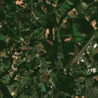
Inputs                                                                                          Ground Truth

                                                                                      …
                 Sentinel                     Road                        OCO-2                                         DARTE
                 Imagery                    Networks                       Data                                        Estimates

                                                                                            Random Crops

                                                       MA-Net

             Channel Stack                                                                     Emissions Prediction

Figure 1: An overview of our process for learning to regress road transport GHG emissions. Primary inputs to our model
include Sentinel-2 satellite imagery (RGB bands only) and road networks from map data, but we also perform experiments
using Orbiting Carbon Observatory-2 (OCO-2) data at 1◦ x 1◦ resolution (≈100 x 100 km), NOAA CarbonTracker (CT)
data, and LandScan population estimates. The ground truth for our experiments is derived from the Database of Road
Transportation Emissions (DARTE) [17], which provides annual bottom-up CO2 estimates at a spatial resolution of 1 km2 .
We crop and interpolate all inputs and ground truth to the resolution of the Sentinel-2 input imagery (10 m ground sample
distance). We train a MA-Net that learns to regress per-pixel CO2 values. This process enables us to improve the spatial
resolution of DARTE estimates, and provide estimates for the specific point in time that the Sentinel-2 imagery was collected.

ison between countries [31, 35]. EDGAR data is available            sector. For example, spectral measurements are commonly
on monthly timescales on a country and sectoral basis [9] or        used to directly measure the presence of GHGs by calcu-
as a 1◦ gridded global annual product. For the road trans-          lating atmospheric absorption features. This can be accom-
portation sector, country or sub-country sectoral emissions         plished readily using ground-based sensors [38, 45], which
are downscaled spatially according to road density.                 are incorporated in some of the aforementioned bottom-
   Recent works, primarily focused the U.S., investigate on-        up approaches. However, more recently, the availability
road GHG emissions. Gately et al. [17], for example, use re-        of spectral-based satellite observations has been increas-
ported vehicular traffic (VHT) data combined with Census            ing [10, 11, 5]. While these systems have been used for
TIGER [34] road network information to estimate regional            direct GHG assessment as early as 1987 [6], only recently
on-road emissions and disaggregate them among mapped                have technological advancements increased the appeal and
road networks.                                                      accessibility of these systems. However, spectral-based
   The “Vulcan Product” is a national-scale, multi-sectoral,        satellite observations still remain fairly coarse in their spa-
hourly inventory from 2010-2015 with a resolution of                tial resolution and temporal frequency. We investigate us-
1 km2 [22]. In this work, transportation emissions are based        ing these observations as model inputs, but they may also
on EPA county-level on-road emissions estimates, which              be beneficial for validating finely-gridded sectoral estimates
are further downscaled using data from the Federal High-            after some spatial aggregation.
way Administration. Gurney et al. also introduced HES-                 Satellite imagery has also been used to estimate GHG
TIA [23], a city-scale produce that uses additional city-           emissions indirectly. Oda et al. [36, 37] demonstrate that vi-
specific data sources to improve inventory accuracy.                sual features, in this case night lights, can be used to disag-
   While these road transportation inventories use bottom-          gregate national emissions and create high-resolution emis-
up methods, there are methods of measuring emissions that           sions estimates grid. Couture et al. [8] present initial works
can be utilized to create inventories of the transportation         towards using visible steam plumes to estimate the oper-

                                                                2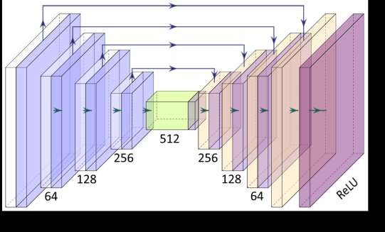
0.45 DARTE Distributions 2017
0.40
0.35
Normalized Frequency
0.30
0.25
0.20
0.15
0.10
0.05
0.00 0 25000 50000 75000 100000 125000 150000 175000 200000
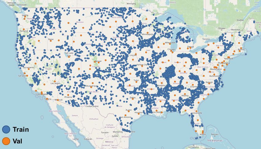
Figure 2: Plot showing city locations sampled from the con- CO2 Concentration (kg CO2/km2)
terminous United States (CONUS) for training (blue) and
validation (orange). Figure 3: Histogram of DARTE road transport CO2 emis-
sions estimates for 2017
ational state of power plants, leading to plant emissions.
Zheng et al. [49] also show that convolutional neural net- data sources and how we use them in our models are de-
works (CNNs) can learn to estimate ground-level PM2.5 , a scribed in the following subsections.
measure of mostly invisible air pollution, from 3-5m res-
olution visible-spectrum PlanetScope imagery [28]. With 3.1.1 Road Transport Emissions
some additional metadata, including weather information,
they show that their model can achieve MAE on the order of Our models learn to regress road transportation CO2 emis-
20%. We take inspiration from these recent efforts in order sions using supervised training with the Database of Road
to create the first global, near-real-time road transportation Transportation Emissions (DARTE) [17]. DARTE provides
emissions inventory. annual (1980-2017) bottom-up CO2 estimates at a spa-
tial resolution of 1 km2 covering the conterminous United
3. Methods States. DARTE leverages the Highway Performance Moni-
toring System, which provides road segments with the fol-
3.1. Data
lowing properties: annual average daily traffic (AADT),
Data is perhaps the most critical component to develop- functional class, urban/rural context, and county. Road seg-
ing a successful approach for top-down road transport emis- ment lengths were combined with AADT to calculate the
sions estimation. Vehicles are small, abundant, and fre- annual vehicle miles travelled (VMT) per segment, which
quently on the move, which makes them especially chal- was partitioned into five vehicle types (passenger cars, pas-
lenging to directly observe. Direct measurement of road senger trucks, buses, single-unit trucks, and combination
transport emissions in a top-down manner would require trucks). A calibrated fuel economy and VMT by vehi-
substantial infrastructure and technological development to cle type were used to calculate motor gasoline and diesel
monitor and track all vehicles. For example, accomplish- fuel consumption, which was smoothed and scaled so that
ing this with Earth observation satellites would require new intra-state values summed to the reported state totals. These
technological advancements addressing spatial resolution, motor gasoline and diesel fuel consumption estimates were
night-time capability, and scalability for continuous moni- then converted to CO2 emissions on an annual basis. For
toring. Currently, many relevant Earth observation systems this initial work we only use DARTE data for 2017, the dis-
are incapable of directly observing periods of peak vehicu- tribution of which is shown in Figure 3.
lar activity (i.e., early morning or late afternoon commutes)
because they operate in sun-synchronous orbits, such as 3.1.2 Visual Imagery
NASA’s Afternoon Constellation [42]. Additionally, many
of these systems do not have sufficient spatial resolution to Visible-spectrum satellite imagery is the primary input for
resolve vehicles. PlanetScope imagery [28], at 3-5 m res- our models. We use Sentinel-2 Level-2A products [14, 18]
olution, seems to be near the limit of what can be used for at 10 x 10 m (100 m2 ) spatial resolution. Level-2A cap-
monitoring vehicles [13, 7]. tures bottom-of-atmosphere reflectance and incorporates
To address these limitations, we investigate leveraging radiometric calibration and orthorectification corrections
various alternative data sources that we hypothesize can be from previous product stages. Sentinel-2 collects 13 spec-
used to indirectly estimate road transport emissions. These tral bands with band centers ranging from approximately
3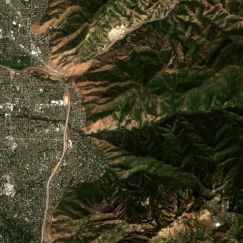
RMSLE: 0.334, MAE: 6.819, MAPE: 0.322

          Image                            Roads                              Ground Truth Emissions                     Predicted Emissions
                                                                                                                                                     700
                                                                                                              250
                                                                                                                                                     600
                                                                                                              200
                                                                                                                                                     500

                                                                                                              150                                    400

                                                                                                                                                     300
                                                                                                              100
                                                                                                                                                     200
                                                                                                              50
                                                                                                                                                     100

Figure 4: Sample results generated by the EN-B3 MA-Net model trained on Sentinel-2 and road data. Colorbars are in units
of kg CO2 per 100 m2 . Roads are colored according to their category: primary road and ramp (red), secondary (green), and
local (blue).

443 nm to 2190 nm. We only use bands 4, 3, and 2 from                        Once Sentinel-2 tiles have been sampled, and before they
each Sentinel-2 image, which roughly correspond to visible                are input into our models, we apply standard ImageNet nor-
red, green, and blue channels, respectively. These bands are              malization and float conversion (intensity ∈ [0, 1]). Auxil-
stacked to form a single 3-channel RGB image, which is                    iary inputs, if any, are then concatenated as additional chan-
also referred to as a true color composite.                               nels in these tile images1 .
   As satellite imagery is the primary input to our model,
we maintain the coordinate reference system (CRS) used                    3.1.3       Roads
by Sentinel-2 Level-2A products and map all auxiliary in-
puts and ground-truth measurements to this CRS. With the                  Road network data is used as an input to our model for three
exception of road data, which is mapped to each swath, all                reasons: 1) it is used to generate bottom-up road trans-
other auxiliary inputs and ground-truth measurements are                  port emissions estimates, 2) their presence should be cor-
mapped to Sentinel-2 imagery on a tile-by-tile basis. In                  related with road transport emissions, and 3) it should be
other words, during training we dynamically extract a more                possible to obtain road network data globally either by us-
manageable subset of each Sentinel-2 swath, which we re-                  ing segmentation models applied to satellite data [46] or by
fer to as a tile, and simultaneously extract all correspond-              sourcing it from governments or open-source databases like
ing auxiliary inputs and ground-truth measurements that fall              OSM [25].
within the bounds of this tile. To account for potential blank               To incorporate road network data, we use Rasterio [19]
regions in each tile, a blank-region mask is created and used             to create GeoTIFFs co-registered with our Sentinel-2
to zero out the corresponding regions from all auxiliary in-              swaths. These GeoTIFFs use road network data extracted
puts and ground truth.                                                    from shapefiles provided by the Census TIGER system [34].
                                                                          Several road categories are provided by Census TIGER, but
    Swaths of Sentinel-2 imagery consist of 10800 x 10800                 we only use data with MAF/TIGER Feature Class Codes
pixels covering approximately 11,664 km2 . A maximum                      (MTFCC) S1100 (primary road), S1630 (ramp), S1200
of 5 Sentinel-2 swaths for each location in our dataset are               (secondary road), and S1400 (local road). Primary road
temporally sampled from the summer (June 1st through                      and ramp categories are merged to form the red channel of
September 30th) of 2017 to minimize the impact of sea-                    each GeoTIFF, while secondary roads and local roads form
sonal changes and occlusion due to weather. To spatially                  the green and blue channels, respectively. These road im-
tile the data, we use a systematic unaligned sampling pro-                ages match the CRS used by our Sentinel-2 swaths and are
cess [12]. The Sentinel-2 swaths are first equally divided                computationally inexpensive to dynamically sample dur-
into an 11x11 grid and then we use this grid as a starting                ing training as Sentinel-2 imagery is tiled. Sample input
point from which a random sub-tile-sized offset is calcu-                 Sentinel-2 and road imagery can be seen in Figure 4.
lated. The combination of a grid intersection and random
offset determine the 1024 x 1024 pixel tile (approximately
105 km2 ) of a Sentinel-2 swath that will be extracted for                3.1.4       CO2
training. The advantage of using this systematic unaligned                The benefits of using additional satellite and ground-based
sampling during the training process is that it maintains an              measurements of CO2 concentrations were also examined
even sampling of tiles from each swath while also introduc-               in this work. The Orbiting Carbon Observatory-2 (OCO-2)
ing a form of data augmentation by not continually sam-
pling identical images.                                                        1 We   do not mask clouds, but intend to explore it in future work.

                                                                     4
satellite from NASA measures column-averaged CO2 dry                population distribution GeoTIFFs from 2000 through 2019.
air mole fraction (XCO2 ) in a sun-synchronous orbit with a         For this effort, we use their 2017 product.
16 day revisit period [11]. To reduce the level of effort in           Each LandScan GeoTIFF contains ambient (24-hour av-
integrating this data into our model, and to address spatial,       erage) population distribution estimates at a roughly 1 km2
temporal, and data quality deficiencies in the OCO-2 Level          spatial resolution. We incorporate these population esti-
2 product [20], we focus on the interpolated OCO-2 Level            mates by extracting tiles co-registered with our Sentinel-2
3 dataset from the University of Wollongong [48]. To cre-           imagery and then concatenating them as an additional chan-
ate the Level 3 product, fixed-rank Kriging is applied with         nel input to our model. Bilinear interpolation is used during
a 16 day moving window in order to create global, daily,            both the CRS resampling process and for any upsampling
CO2 concentration estimates. Tabulated Level 3 products             needed to match the Sentinel-2 tile resolution. To ensure
were first converted to global, annually-averaged GeoTIFFs          population consistency before and after this processing pro-
for easier integration into the data processing pipeline. Due       cedure, we normalize the resampled population tile to en-
to the lower 1◦ x 1◦ (≈100 x 100 km, depending on lati-             sure that its total population matches the population total of
tude) spatial resolution of the OCO-2 Level 3 product, typ-         the same region before resampling. Sample population data
ically only a single OCO-2 measurement covers an entire             can be seen in Figure 5.
Sentinel-2/DARTE tile (≈10 x 10 km). Thus, this value is
used for all input image pixels in the form of an additional
input channel.                                                      3.1.6   Dataset Partitioning
    Ground-based CO2 measurements were also explored                The dataset we created for this work was constructed from
in order to determine whether measurements taken closer             data (e.g., satellite imagery, roads, etc.) depicting 3753
to road-level offered any measurable improvement in                 cities for training and 118 cities for validation, as visualized
emissions estimation accuracy. NOAA’s CarbonTracker                 in Figure 2. These cities are isolated to the conterminous
project [38] offers monthly-averaged CO2 mole fraction es-          United States (covering over 8 Mkm2 ).
timations at 1◦ x 1◦ spatial resolution over North America,             Since the U.S. is vast and contains many sparsely popu-
and at varying levels of the atmosphere [30]. These concen-         lated regions, we construct our dataset by targeting regions
trations are derived from their optimized surface flux prod-        that are most likely to have roads. We accomplish this by
uct that incorporates 460 observation datasets from across          first creating a list of cities from the United States Cities
the globe, recorded on the ground, in aircraft, and on-             Database [33], which is an aggregation of data collected by
board ships. Concentrations are available at 26 geopoten-           the U.S. Geological Survey and U.S. Census Bureau. Next,
tial heights, but we use values closest to the ground with an       we designate cities for the validation split by identifying the
average altitude of 445 m. Similar to OCO-2, an annual av-          nearest neighboring city to 108 airports across the U.S. [44],
erage GeoTIFF is created and a single CarbonTracker value           where at least one city is selected for each state. Since air-
is used as an additional channel for each input tile.               ports tend to be spatially dispersed across the U.S., the cities
                                                                    set aside for the validation set reflect many of the diverse
3.1.5   Population                                                  geographies across the U.S.
                                                                        With validation cities identified, we construct the train-
Population is likely to be correlated with road transport           ing split by removing all cities within a 120 km radius of
emissions, as vehicles are still primarily operated by peo-         the centerpoint of any validation city. This process prevents
ple and there were 1.88 vehicles per household as of 2001-          potential overlap in imagery across dataset splits. We then
2007 [2]. As such, we investigated incorporating population         down-select from this filtered list, iterating over each state
data into our model as an additional channel input. There           and omitting all cities not included in the 35 most popu-
are several sources of population data, with the most accu-         lated cities, the 35 least populated cities, and 30 randomly-
rate source likely coming from a governmental censuses.             selected remaining cities. Should a state not have 100 cities
However, our eventual goal for this work is to estimate             in total, all cities are selected.
road transport emissions globally, in a top-down manner,                After partitioning the cities, we can begin to load tile
and without reliance on extensive data collection from local        tuples (i.e., co-registered data across our various sources)
governments.                                                        for training our models. However, as we load tiles we can
   It is possible to achieve reasonable accuracy by estimat-        encounter conditions that are not ideal for training machine
ing population from overhead imagery [24]. For this effort,         learning models. If 50% or more of a DARTE tile contains
we require annual (or sub-annual) gridded population esti-          invalid data then we filter the tuple. Similarly, if more than
mates that can be paired with Sentinel-2 and DARTE data.            20% of a Sentinel-2 tile is empty then we filter the tuple.
LandScan estimates [41] provided by Oak Ridge National              We also filter out any tiles associated with data read errors.
Laboratory meet this need. LandScan offers annual global                After these filtering processes, we are left with 297,296

                                                                5
Method RMSLE MAE MAPE Method RMSLE MAE MAPE
RN-34 U-Net 0.661 38.9 50% S2 1.03 55.9 65%
EN-B3 U-Net 0.71 51.2 47% R 0.73 43.3 64%
EN-B3 Reduced U-Net 0.836 2669 214% S2+R 0.616 39.5 55%
EN-B3 MA-Net 0.616 39.5 55% S2+OCO2 1.05 55.1 88%
S2+R+LS 0.739 49.9 47%
Table 1: Comparison of results across varying neural net- S2+R+OCO2 0.709 49.3 46%
work architectures trained on Sentinel-2 and road network S2+R+OCO2+CT 0.817 52.6 46%
data, including ResNet-34 (RN-34) and EfficientNet-B3
(EN-B3) backbone U-Nets, a Reduced U-Net architecture, Table 2: Comparison of MA-Net results for models trained
and an MA-Net architecture. MAE is in units of kg CO2 with varying inputs, including Sentinel-2 visual imagery
per 100 m2 . (S2), road imagery (R), LandScan (LS) population esti-
mates, Orbiting Carbon Observatory-2 (OCO2) Level 3
data, and CarbonTracker data (CT). MAE is in units of kg
tiles (over 31 Mkm2 ) for training and 45,224 tiles (over CO2 per 100 m2 .
4.7 Mkm2 ) for validation. We further split our validation
tiles into a random subset of 1000 tiles that are used to val-
idate each epoch during model training and select optimal tion, etc.) along with different loss functions. We found the
model weights, as well as 44,224 testing tiles that are used normalization approaches offered little benefit, while root
to generate the results in Tables 1 and 2. mean square logarithmic error (RMSLE) and mean absolute
percentage error (MAPE) loss functions were more promis-
3.2. Architecture ing. We believe this is likely due to large variations and
The two base architectures we used in our experiments outliers in road transport emissions across varying geogra-
were U-Net [40] and MA-Net [16]. U-Nets have been a phies, as illustrated in the histogram of DARTE emissions
popular choice for the winning solutions of several pub- data in Figure 3. For example, many rural areas have few
lic challenges and datasets focused on per-pixel classifica- roads and relatively little road transport emissions. Con-
tion and regression in both medical imaging (where they versely, dense cities have high road densities and road trans-
were conceived) and satellite imagery [4, 46, 21]. Both port emissions. Furthermore, city emissions can vary dra-
ResNet-34 [26] and EfficientNet-B3 [43] backbones were matically depending on factors such as public transit usage.
tested. Given that DARTE data has a lower resolution than RMSLE is commonly used for regression tasks where
Sentinel-2 imagery (1 km2 vs 100 m2 ), we also decided to the underlying ground truth data distribution is exponential
modify the standard U-Net to perform reduced upsampling or has many outliers, expressed as follows:
within the network. Given that inputs to the network had a
1024 x 1024 resolution, we only kept enough upsampling v
u n
layers to result in an output size of 128 x 128, which is u1 X
RM SLE = t (log(Pi + 1) − log(GTi + 1))2 .
closer to the native DARTE resolution for a crop of the same n i=1
geographic region. We refer to this architecture as the “Re- (1)
duced U-Net”. Given the shared success of U-Nets in both Our mean absolute percentage error (MAPE) metric is
the medical imaging and satellite imagery domains, we also slightly modified from the typical MAPE equation to im-
decided to test the MA-Net architecture due to its recent prove numerical stability as the ground truth (GT ) ap-
success in tumor segmentation applications. proaches 0, which is defined as:
All model architecture and backbone implementations
n
used in this work were built upon the implementations of 100 X |(GTi + 1) − (Pi + 1)|
[47]. With each model using a ReLU activation for its final M AP E = . (2)
n i=1 GTi + 1
layer to regress positive per-pixel CO2 values. Additionally,
RAdam [32] was used as the optimizer of choice for our ex- In each equation, n represents the number of pixels in
periments with a learning rate of 1e-3, betas of (0.9, 0.999), each tile, i represents the pixel index, P represents the pre-
and eps of 1e-8. dicted emissions output from our model, and GT represents
the upsampled ground-truth emissions from DARTE.
3.3. Loss functions
In our experiments, we achieved the best performance
We experimented with different procedures for normal- by training using an RMSLE loss function. One added ben-
izing the DARTE data (e.g., 0-1 normalization, mean-std efit to using RMSLE in the context of emissions estima-
normalization, quantile transformation, K-bins discretiza- tion is that RMSLE is biased towards overestimating. In
6other words, underestimates incur a larger cost than over- of these input data sources. Sample results from these mod-
estimates. In the context of mitigating climate change, it is els can be seen in Figure 5. The best performing model
safer to overestimate emissions and take more drastic ac- was trained using Sentinel-2 imagery and road network
tion than necessary as opposed to underestimating emis- data. This model outperformed both the Sentinel-2 only and
sions and not taking sufficient action. Roads-only models, as we expected. However, results from
models trained with additional inputs from OCO-2, Land-
4. Results & Discussion Scan, and CarbonTracker all underperform compared to the
model using only Sentinel-2 and road data. We hypothe-
We evaluate multiple segmentation architectures and size that this may also be related to the spatial resolution
backbones against our reduced Sentinel-2 and roads dataset mismatch, except in this instance not only is there a mis-
to obtain the results shown in Table 1. An MA-Net ar- match between the inputs and our ground truth but there is
chitecture with EfficientNet-B3 backbone achieves the best a mismatch between different input data sources. Road data
results with an RMSLE of 0.616, while ResNet-34 and is actually rasterized to match the spatial resolution of the
EfficientNet-B3 backboned U-Nets achieve slightly better input Sentinel-2 data, whereas all other input data sources
MAE and MAPE. have different underlying resolutions. It is possible that this
We believe one of the biggest challenges associated with spatial resolution mismatch between input data sources in-
training these models comes from the spatial resolution mis- troduces an additional challenge by implying certain image
match between our predictions and the ground truth. Fig- regions are more similar than the higher-resolution data in-
ures 4 and 5 qualitatively illustrate that our EfficientNet-B3 dicates. Late fusion or other techniques that account for this
backbone MA-Net model is capable of learning that road mismatch may need to be investigated to improve exploita-
transport emissions are highest on roads. Taking notice of tion of these inputs.
the the bright yellow region near the bottom-center of the Another aspect to consider in reviewing our model re-
“Predicted Emissions” image. Instead of reproducing the sults is the overall difficulty of our dataset. The included
blurry yellow region of emissions located at the same region cities and neighboring regions contain diverse geographies
in the “Ground Truth Emissions” image, this model can pre- and 5 of the 6 Köppen-Geiger climate zone types, which can
dict large emissions with fine-grained structure matching be visually representative of many regions across the globe.
the roads present in the scene. However, by calculating error This visual diversity adds challenge, but also helps inform
in a pixel-wise fashion, the model is penalized for learning the ability of the model to generalize globally.
this fine-grained structure. In other words, if the model cor- Additionally, as shown in Figure 2, our validation split
rectly estimates low emissions from nearby farmland, it will sequesters many of the largest east and west-coast cities
be penalized due to the fact that our ground truth contains from training. Many of these cities represent significant
large emissions values in that area. outliers, both visually and in terms of their emissions, com-
We believe that one potential solution for this spatial res- pared to most other U.S. cities. However, the challenge
olution mismatch is to compare model predictions at the of this split may also offer insight towards global gener-
same resolution as the ground truth. Our Reduced U-Net alizability. Road transport emissions estimation methods
architecture represents a first attempt to accomplish this. must learn to generalize not only across diverse visual back-
Rather than outputting 1024 x 1024 pixel predictions that grounds, as discussed previously, but also across diverse ar-
matches the spatial resolution of its input, our Reduced U- chitectures, population densities, and transport systems lo-
Net outputs a 128 x 128 prediction to more closely match cated across small, medium, and large cities.
the spatial resolution of our ground truth. Unfortunately, A similar point can also be made concerning our data
as can be seen in Table 1, this approach does not perform sampling procedure. The population density or urbaniza-
well, resulting in significantly higher RMSLE, MAE, and tion distribution of tiles in our dataset is likely skewed,
MAPE. We hypothesize that the poor performance of this matching the real world distribution. However, for the
model is due, at least in part, to the reduction of skip con- purposes of training a model that can estimate urban road
nections, especially from high-resolution layers, which may transport emissions as accurately as rural road transport
be necessary to exploit the small and subtle visual features emissions, it may be necessary to oversample the less-
(e.g., roads, buildings, etc.) in our imagery. We suspect frequently-occuring urban areas, especially as estimating
that simply adding additional downsampling layers after the urban road transport emissions is likely to be a more chal-
segmentation architecture may perform better, but leave this lenging task.
experiment for future work.
In Section 3, we outline several data sources that we 5. Conclusion
believe may improve our model’s accuracy and ability to
generalize. As shown in Table 2, we trained multiple We present the first published automated approach for
EfficientNet-B3 MA-Net models on varying permutations estimating road transport sector emissions in a top-down
7Sentinel-2 Roads Population
0.8
0.6
0.4
0.2
0.0
S2 R S2 + R
DARTE Ground Truth MAE: 312.008 MAE: 226.710 MAE: 190.016
2000 100 600
500 1250
1500 80
400 1000
60 750
1000 300
40 200 500
500 20 100 250
0 0 0 0
S2 + OCO2 S2 + R + LS S2 + R + OCO2 S2 + R + OCO2 + CT
MAE: 311.561 MAE: 253.414 MAE: 266.012 MAE: 280.997 300
800 600
120 250
100 500
600 200
80 400
400 300 150
60
40 200 100
200
20 100 50
0 0 0 0
Figure 5: Example results from the seven models listed in Table 2. Emissions colorbars are in units of kg CO2 per 100 m2 ,
and LandScan population is in units of people per 100 m2 .
fashion using visual satellite imagery. Using primarily time road transportation emissions inventories that can pro-
Sentinel-2 imagery and road network data over the conter- vide independent and objective feedback as the global com-
minous United States, we train an MA-Net segmentation munity tackles climate change.
model to regress road transport emissions on a pixel-by-
pixel basis using an RMSLE loss. Our model achieves an 6. Acknowledgements
MAE of 39.5 kg CO2 per 100 m2 .
This research was conducted as part of the Climate
Significant challenges remain to operationalize this tech- TRACE initiative to track global GHG emissions and make
nology. Model accuracy must be improved and estima- the data publicly available. Financial support was provided
tion uncertainty quantified to provide actionable informa- by a grant from Generation Investment Management. We
tion for regional governments and municipalities. The lim- would also like to thank Gabriela Volpato and Aaron Davitt
ited availability of accurate and global road transportation from WattTime, as well as Mathieu Carlier, Bénédicte De
emissions data must be overcome, including concerns of Gelder, and Alain Retière from Everimpact for their sup-
model transfer and regional bias. It remains to be seen if port identifying data sources and discussing methodology.
changes in government policy and human behavior over an-
nual timescales will be captured by our models, although References
this hypothesis will be testable as data from 2020 emerges. [1] Revision of the UNFCCC reporting guidelines on annual in-
Despite these challenges, we believe this work represents ventories for Parties included in Annex I to the Convention.
a critical step towards building scalable, global, near-real- UNFCCC, 2013. 1
8[2] 2017 national household travel survey: Summary of travel et al. Sentinel-2: ESA’s optical high-resolution mission for
trends. Technical report, U.S. Department of Transportation: GMES operational services. Remote sensing of Environment,
Federal Highway Administration, 2017. 5 2012. 3
[3] Inventory of U.S. Greenhouse Gas Emissions and Sinks: [15] HS Eggleston, Leandro Buendia, Kyoko Miwa, Todd Ngara,
1990-2018. Technical report, U.S. Environmental Protection and Kiyoto Tanabe. 2006 IPCC guidelines for national
Agency, 2020. 1 greenhouse gas inventories. 2006. 1
[4] Marc Bosch, Kevin Foster, Gordon Christie, Sean Wang, [16] Tongle Fan, Guanglei Wang, Yan Li, and Hongrui Wang.
Gregory D Hager, and Myron Brown. Semantic stereo for Ma-net: A multi-scale attention network for liver and tumor
incidental satellite images. In WACV, 2019. 6 segmentation. IEEE Access, 2020. 6
[5] Michael Buchwitz, Markus Reuter, O Schneising, Hartmut [17] Conor K Gately, Lucy R Hutyra, and Ian Sue Wing. Cities,
Boesch, Sandrine Guerlet, B Dils, Ilse Aben, R Armante, P traffic, and co2 : A multidecadal assessment of trends,
Bergamaschi, Thomas Blumenstock, et al. The Greenhouse drivers, and scaling relationships. Proceedings of the Na-
Gas Climate Change Initiative (GHG-CCI): Comparison and tional Academy of Sciences, 2015. 1, 2, 3
quality assessment of near-surface-sensitive satellite-derived [18] A Gatti and A Bertolini. Sentinel-2 products specification
CO2 and CH4 global data sets. Remote Sensing of Environ- document, 2015. 3
ment, 2015. 2 [19] Sean Gillies et al. Rasterio: geospatial raster i/o for Python
[6] Alain Chédin, Anthony Hollingsworth, Noelle A Scott, programmers, 2013–. 4
Soumia Serrar, Cyril Crevoisier, and Raymond Armante. An- [20] OCO-2 Science Team/Michael Gunson and Annmarie Elder-
nual and seasonal variations of atmospheric CO2, N2O and ing. OCO-2 Level 2 bias-corrected XCO2 and other select
CO concentrations retrieved from NOAA/TOVS satellite ob- fields from the full-physics retrieval aggregated as daily files,
servations. Geophysical research letters, 2002. 2 Retrospective processing V9r, 2018. 5
[7] Yulu Chen, Rongjun Qin, Guixiang Zhang, and Hessah Al- [21] Ritwik Gupta, Bryce Goodman, Nirav Patel, Ricky Hosfelt,
banwan. Spatial Temporal Analysis of Traffic Patterns dur- Sandra Sajeev, Eric Heim, Jigar Doshi, Keane Lucas, Howie
ing the COVID-19 Epidemic by Vehicle Detection Using Choset, and Matthew Gaston. Creating xbd: A dataset for as-
Planet Remote-Sensing Satellite Images. Remote Sensing, sessing building damage from satellite imagery. In CVPRW,
2021. 3 2019. 6
[8] Heather Couture, Joseph O’Connor, Grace Mitchell, Isabella [22] Kevin R Gurney, Jianming Liang, Risa Patarasuk, Yang
Söldner-Rembold, Durand D’souza, Krishna Karra, Keto Song, Jianhua Huang, and Geoffrey Roest. The Vulcan ver-
Zhang, Ali Rouzbeh Kargar, Thomas Kassel, Brian Gold- sion 3.0 high-resolution fossil fuel CO2 emissions for the
man, Daniel Tyrrell, Wanda Czerwinski, Alok Talekar, and United States. Journal of Geophysical Research: Atmo-
Colin McCormick. Towards tracking the emissions of every spheres, 2020. 1, 2
power plant on the planet. NeurIPS Workshop, 2020. 2 [23] Kevin R Gurney, Igor Razlivanov, Yang Song, Yuyu Zhou,
[9] Monica Crippa, Efisio Solazzo, Ganlin Huang, Diego Guiz- Bedrich Benes, and Michel Abdul-Massih. Quantification
zardi, Ernest Koffi, Marilena Muntean, Christian Schieberle, of fossil fuel co2 emissions on the building/street scale for a
Rainer Friedrich, and Greet Janssens-Maenhout. High reso- large us city. Environmental science & technology, 2012. 2
lution temporal profiles in the emissions database for global [24] Armin Hadzic, Gordon Christie, Jeffrey Freeman, Amber
atmospheric research. Scientific data, 7(1):1–17, 2020. 2 Dismer, Stevan Bullard, Ashley Greiner, Nathan Jacobs, and
[10] David Crisp, RM Atlas, F-M Breon, LR Brown, JP Burrows, Ryan Mukherjee. Estimating displaced populations from
P Ciais, BJ Connor, SC Doney, IY Fung, DJ Jacob, et al. overhead. arXiv preprint arXiv:2006.14547, 2020. 5
The orbiting carbon observatory (OCO) mission. Advances [25] Mordechai Haklay and Patrick Weber. Openstreetmap: User-
in Space Research, 2004. 2 generated street maps. IEEE Pervasive computing, 2008. 4
[11] David Crisp, Harold R Pollock, Robert Rosenberg, Lars [26] Kaiming He, Xiangyu Zhang, Shaoqing Ren, and Jian Sun.
Chapsky, Richard AM Lee, Fabiano A Oyafuso, Chris- Deep residual learning for image recognition. In CVPR,
tian Frankenberg, Christopher W O’Dell, Carol J Bruegge, 2016. 6
Gary B Doran, et al. The on-orbit performance of the Orbit- [27] Leif Hockstad and L Hanel. Inventory of us greenhouse
ing Carbon Observatory-2 (OCO-2) instrument and its radio- gas emissions and sinks. Technical report, Environmental
metrically calibrated products. Atmospheric Measurement System Science Data Infrastructure for a Virtual Ecosystem,
Techniques, 2017. 2, 5 2018. 1
[12] Eric Delmelle. Spatial sampling. The SAGE handbook of [28] Planet Labs Inc. Planet imagery product specifications,
spatial analysis, 2009. 4 2020. 3
[13] Sébastien Drouyer. Parking occupancy estimation on plan- [29] World Resource Institute. Climate watch historical ghg emis-
etscope satellite images. In IGARSS 2020-2020 IEEE Inter- sions. https://www.climatewatchdata.org/
national Geoscience and Remote Sensing Symposium, pages ghg-emissions, 2020. 1
1098–1101. IEEE, 2020. 3 [30] Andrew R. Jacobson et al. CarbonTracker CT2019B, 2020.
[14] Matthias Drusch, Umberto Del Bello, Sébastien Carlier, 5
Olivier Colin, Veronica Fernandez, Ferran Gascon, Bianca [31] Greet Janssens-Maenhout, Monica Crippa, Diego Guizzardi,
Hoersch, Claudia Isola, Paolo Laberinti, Philippe Martimort, Marilena Muntean, Edwin Schaaf, Frank Dentener, Peter
9Bergamaschi, Valerio Pagliari, Jos GJ Olivier, Jeroen AHW Wennberg, Brian Connor, Vanessa Sherlock, David Griffith,
Peters, et al. EDGAR v4.3.2 Global Atlas of the three major Nick Deutscher, et al. Total column carbon observing net-
Greenhouse Gas Emissions for the period 1970–2012. Earth work (tccon). In Fourier Transform Spectroscopy, 2009. 2
System Science Data Discussions, 2017. 1, 2 [46] Adam Van Etten, Dave Lindenbaum, and Todd M Bacastow.
[32] Liyuan Liu, Haoming Jiang, Pengcheng He, Weizhu Chen, Spacenet: A remote sensing dataset and challenge series.
Xiaodong Liu, Jianfeng Gao, and Jiawei Han. On the vari- arXiv preprint arXiv:1807.01232, 2018. 4, 6
ance of the adaptive learning rate and beyond. arXiv preprint [47] Pavel Yakubovskiy. Segmentation models pytorch. https:
arXiv:1908.03265, 2019. 6 //github.com/qubvel/segmentation_models.
[33] Pareto Software LLC. simplemaps: United states cities pytorch, 2020. 6
database, 2021. 5 [48] Andrew Zammit-Mangion, Noel Cressie, and Clint Shu-
[34] Robert W Marx. The TIGER system: automating the geo- mack. On statistical approaches to generate level 3 prod-
graphic structure of the United States census. Government ucts from satellite remote sensing retrievals. Remote Sensing,
publications review, 1986. 2, 4 2018. 5
[35] M Muntean, D Guizzardi, E Schaaf, M Crippa, E Solazzo, [49] Tongshu Zheng, Michael H Bergin, Shijia Hu, Joshua Miller,
J Olivier, and E Vignati. Fossil CO2 emissions of all world and David E Carlson. Estimating ground-level PM2.5 using
countries. Luxembourg: Publications Office of the European micro-satellite images by a convolutional neural network and
Union, 2018. 2 random forest approach. Atmospheric Environment, 2020. 3
[36] Tomohiro Oda and Shamil Maksyutov. A very high-
resolution (1 km× 1 km) global fossil fuel CO2 emission
inventory derived using a point source database and satellite
observations of nighttime lights. Atmospheric Chemistry and
Physics, 2011. 2
[37] Tomohiro Oda, Shamil Maksyutov, and Robert J Andres.
The Open-source Data Inventory for Anthropogenic CO2 ,
version 2016 (ODIAC2016): a global monthly fossil fuel
CO2 gridded emissions data product for tracer transport sim-
ulations and surface flux inversions. Earth System Science
Data, 2018. 2
[38] Wouter Peters, Andrew R Jacobson, Colm Sweeney, Ar-
lyn E Andrews, Thomas J Conway, Kenneth Masarie, John B
Miller, Lori MP Bruhwiler, Gabrielle Pétron, Adam I Hirsch,
et al. An atmospheric perspective on North American car-
bon dioxide exchange: CarbonTracker. Proceedings of the
National Academy of Sciences, 2007. 2, 5
[39] Sims R., R. Schaeffer, X. Cruz-Núñez F. Creutzig, M.
D’Agosto, D. Dimitriu, M.J. Figueroa Meza, L. Fulton, S.
Kobayashi, O. Lah, A. McKinnon, P. Newman, M. Ouyang,
J.J. Schauer, D. Sperling, and G. Tiwari. Transport. In Cli-
mate Change 2014: Mitigation of Climate Change. Contri-
bution of Working Group III to the Fifth Assessment Report
of the Intergovernmental Panel on Climate Change. Cam-
bridge University Press, Cambridge, United Kingdom and
New York, NY, USA, 2014. 1
[40] Olaf Ronneberger, Philipp Fischer, and Thomas Brox. U-net:
Convolutional networks for biomedical image segmentation.
In MICCAI, 2015. 6
[41] Amy N. Rose, Jacob J. McKee, Marie L. Urban, and Ed-
die A. Bright. Landscan 2017, 2018. CY 2017. 5
[42] Mark R Schoeberl. The afternoon constellation: a formation
of earth observing systems for the atmosphere and hydro-
sphere. In IGARSS, 2002. 3
[43] Mingxing Tan and Quoc Le. Efficientnet: Rethinking model
scaling for convolutional neural networks. In ICML, 2019. 6
[44] Orogo Technologies. Latitude-longitude of us cities
(www.realestate3d.com), 1997. 5
[45] Geoffrey Toon, Jean-Francois Blavier, Rebecca Washen-
felder, Debra Wunch, Gretchen Keppel-Aleks, Paul
10You can also read