1813 Do Energy Effi ciency Networks Save Energy? Evidence from German Plant-Level Data - DIW Berlin

1813
Discussion
Papers

Deutsches Institut für Wirtschaftsforschung 2019

Do Energy Efficiency Networks
Save Energy? Evidence from
German Plant-Level Data

Jan Stede

Opinions expressed in this paper are those of the author(s) and do not necessarily reflect views of the institute.

IMPRESSUM

© DIW Berlin, 2019

DIW Berlin
German Institute for Economic Research
Mohrenstr. 58
10117 Berlin

Tel. +49 (30) 897 89-0
Fax +49 (30) 897 89-200
http://www.diw.de

ISSN electronic edition 1619-4535

Papers can be downloaded free of charge from the DIW Berlin website:
http://www.diw.de/discussionpapers

Discussion Papers of DIW Berlin are indexed in RePEc and SSRN:
http://ideas.repec.org/s/diw/diwwpp.html
http://www.ssrn.com/link/DIW-Berlin-German-Inst-Econ-Res.html

Do energy efficiency networks save energy? Evidence from German plant-
 level data

 Jan Stede*

Abstract: In energy efficiency networks, groups of firms exchange experiences on energy
conservation in regular meetings over several years. The companies implement energy efficiency
measures in order to reach commonly agreed energy savings and CO2 reduction goals. Energy
efficiency networks exist in several countries, such as Germany, Sweden and China. Existing
evaluations of such voluntary regional networks in Germany claim that participants improved
energy efficiency at twice the speed of the industry average. Based on comprehensive data from the
German manufacturing census, this paper examines whether participation in energy efficiency
networks has a causal impact on energy conservation and CO2 emissions. I employ both a
difference-in-differences estimator, using companies that joined energy efficiency networks at a
later point in time as a control group, as well as a semiparametric matching estimator. I demonstrate
that for the average participant there is no evidence of a statistically significant effect on energy
productivity or CO2 emissions due to the network activities. However, there is some indication that
exporters may have benefitted from the networks by reducing their CO2 emissions.

Keywords: Business networks; voluntary agreements; energy conservation; policy evaluation
JEL codes: D22; Q40; Q51; C50

________________
* German Institute for Economic Research (DIW Berlin), Climate Policy Department,
Mohrenstr. 58, 10117 Berlin, Germany. jstede@diw.de.

1 Introduction
Energy efficiency is often seen as a cost-effective way to reduce greenhouse gas emissions in order
to contain global warming (IEA, 2018; IPCC, 2018). However, there is an “energy efficiency gap”
(Jaffe and Stavins, 1994), due to a range of market failures and investment barriers such as
behavioural anomalies (Gillingham and Palmer, 2014). Energy efficiency policies correcting for
market failures and underinvestment may therefore play a key role in meeting the 2°C target agreed
in the landmark Paris Agreement. A significant share of energy saving opportunities are in the
industrial sector, which accounts for almost 30 per cent of final energy consumption in Germany
and 26 per cent in the European Union (AGEB, 2016; Lapillonne and Sudries, 2016).

Energy efficiency networks are voluntary agreements of companies, targeted at reducing energy
consumption in industry. In such networks, 10 to 15 firms from different economic sectors
exchange experiences at regular moderated meetings over a period of 3-4 years in order to achieve
jointly agreed energy efficiency and CO2 savings targets (Jochem and Gruber, 2007; Köwener et al.,
2014; Rohde et al., 2015). The basic mechanism through which energy efficiency networks operate
is an information treatment, encouraging investment into energy efficiency by providing companies
with the knowledge and skills to effectively reduce energy consumption. Energy efficiency
networks are typically regional. They focus on efficiency improvements in cross-sectional
technologies (such as lighting or process heat), since participating companies come from different
economic sectors with different production technologies (Jochem et al., 2010). Originating from
Switzerland, energy efficiency networks now exist in several OECD and large non-OECD
countries, such as Germany, Sweden and China (Jochem et al., 2016; Paramonova and Thollander,
2016; OECD/IPEEC, 2017).

In Germany, energy efficiency networks are one of the major instruments in the national policy
mix to improve energy efficiency in industry and reach national climate targets. Together with the
main industrial associations, the German government plans to create 500 networks by 2020,
delivering savings of up to five million tonnes of CO2 through voluntary agreements (Barckhausen
et al., 2018; BMU, 2019). These savings would account for 1/5 of all measures that reduce energy
consumption set out in Germany’s “National Action Plan on Energy Efficiency” (NAPE), which
are necessary to comply with the EU Energy Efficiency Directive (Ringel et al., 2016).

Energy efficiency networks in Germany are generally considered a success in the existing literature.
Most studies have looked at the so-called German “pilot networks”, which were carried out
between 2009 and 2014, before the official adoption of the target of setting up 500 networks.
More than 360 companies have participated in 30 of these initial energy efficiency networks. The
literature on these networks has focused on bottom-up calculations of energy savings achieved
during the networking period, as well as surveys among participating companies (see, e.g.,
Wohlfarth et al., 2016; Barckhausen et al., 2018; Dütschke et al., 2018). Some of these evaluations
conclude that participating companies increased their energy efficiency at two per cent or double
the speed of the industrial sector as a whole (Jochem et al., 2010; Köwener et al., 2014; Rohde et
al., 2015). However, survey evidence also suggests that a large chunk of these energy conservation
measures may not have been additional, since the firms would have carried out these measures
anyways (e.g. Wohlfarth et al., 2016).

 1

The main contribution of this paper is that it is the first to use plant-level data in order to uncover
whether there is a causal relationship between participation in an energy efficiency network and
increased energy efficiency, as well as reduced CO2 emissions. I use two different estimation
strategies to explore this causal link. First, I employ a difference-in-differences estimator,
comparing the energy productivity and CO2 emissions of participants of the pilot phase 2009-2014
(treatment group) to a group of plants joining German energy efficiency networks that were
initiated after the pilot networks had been completed (post-2014). These latter firms also chose to
become part of an efficiency network, but did not receive the treatment until the pilot phase was
over. Relative to the average manufacturing firm, this control group is much more similar to the
participants of the pilot networks in terms of observables such as average energy consumption or
number of employees.

I find no evidence of a statistically significant effect of the energy efficiency networks on either
energy productivity or CO2 emissions for the average plant. While in some specifications there is a
statistically and economically significant effect of the networks on energy productivity and CO2
emissions, this effect is driven by a few large installations. In the most robust specifications, there is
no evidence of an effect of the networks. I provide visual support for the identifying assumption
of parallel trends of treatment and control group in the absence of the treatment. Moreover, I test
for anticipation effects and do not find evidence of either an increased energy productivity or
lower CO2 emissions prior to the uptake of a network. This lends additional credibility to the
identifying assumption.

In order to check the robustness of these results, I employ a semiparametric matching estimator in
a second step. This estimator aligns the distribution of observed variables of treatment and control
group that are relevant for energy conservation efforts by choosing appropriate comparison units
from the entire manufacturing sector. This reduces the differences between treatment and control
group in terms of observables. Moreover, by taking first differences, the estimator accounts for
selection on time-invariant plant characteristics, such as organisational structures that favour energy
efficiency investments. Results from the matching estimation support the finding of no significant
treatment effect due to the network activities. My results are in stark contrast to previous
assessments of energy efficiency networks in Germany, and highlight the importance of ex-post
policy evaluation.

Finally, I explore heterogeneous treatment effects by taking a closer look at network participants
with high exports. I find some indication that high exporters may benefit from energy efficiency
networks by reducing their CO2 emissions. This result may be explained by a better management of
exporting firms, which allows exporters to profit more from participating in energy efficiency
networks than the average industrial firm. Exporting firms have been found to be more innovative
and more productive than domestic non-exporters (Helpman et al., 2004; Yeaple, 2005; Aw et al.,
2008; Lileeva and Trefler, 2010). Moreover, exporting may improve management practices (Bloom
and Van Reenen, 2010), which in turn may have positive spillovers on energy efficiency (Bloom et
al., 2010; Martin et al., 2012; Boyd and Curtis, 2014). Exporting German manufacturers in
particular have been found to be more energy efficient than their non-exporting counterparts (Lutz
et al., 2017).

This research contributes to the literature on the impact evaluation of voluntary environmental
management programmes using firm-level data. Voluntary agreements to reduce the environmental
 2

impacts of production processes have received increasing attention (Segerson and Miceli, 1998),
with mixed results on their effectiveness. Well-studied voluntary programmes include the U.S.
Environmental Protection Agency’s 33/50 (Arora and Cason, 1995; Khanna and Damon, 1999;
Gamper-Rabindran, 2006; Vidovic and Khanna, 2007; Carrión-Flores et al., 2013), as well as the
norm for environmental management systems ISO 14001 (e.g. Arimura et al., 2011; see also the
comprehensive overview by Boiral et al., 2018). European voluntary programmes such as the EU’s
Eco Management and Audit Scheme (EMAS), on the other hand, have received considerably less
attention (e.g. Bracke et al., 2008). Recently, Kube et al. (2019) find no effect of EMAS on either
CO2 intensity, energy intensity or investments for German manufacturing firms.

The paper is structured as follows. Section 2 explains the concept of energy efficiency networks, as
well as the mechanisms through which they are thought to help energy conversation. It also
describes the pilot phase of energy efficiency networks in Germany. Section 3 outlines two
alternative identification strategies used to estimate the treatment effect of energy efficiency
networks. Section 4 portrays the panel dataset used in this study, discusses the use of energy
productivity as an indicator for energy efficiency, and provides descriptive statistics. Section 5
presents the results and discusses the identifying assumptions. Section 6 concludes.

2 Energy efficiency networks – how they work
Energy efficiency networks (EENs) are an attempt to overcome investment barriers to energy
efficiency within companies. EENs work on a voluntary basis, but are often incentivised by existing
regulatory and policy frameworks (OECD/IPEEC, 2017). The networks are typically regional,
meaning that companies from different sectors within one region may join the same network. The
cross-sectoral nature of regional energy efficiency networks addresses concerns over sharing
sensitive information with potential competitors (Jochem et al., 2010). However, other types of
networks also exist. Sectoral networks are made up of different firms from the same sector.
Internal company networks, on the other hand, comprise different manufacturing sites of a parent
company that join an organisation-wide energy efficiency network.

Figure 1 illustrates how energy efficiency networks work.1 During an initial identification phase
(phase 1), profitable energy saving opportunities are identified in an energy audit. Each network
participant then commits to a voluntary energy savings goal, as well as a CO2 reduction goal. The
individual goals add up to a joint network target. In the networking phase (phase 2), participants
meet at regular moderated meetings for three to four years. Here, they share their experience about
the implementation of energy efficiency measures. Moreover, external experts provide input on
topics such as energy efficiency technologies, organisational measures like awareness raising among
employees, or financing of energy efficiency investments. There are also yearly site visits to
monitor progress towards the energy efficiency goal and, at the same time, to allow participants to
see efficiency measures implemented in other companies.

1 Figure 1 is based on the LEEN standard (“Learning energy efficiency networks”), a voluntary quality standard on how
to establish and run energy efficiency networks, including a standardised monitoring of the energy savings achieved.
LEEN was developed during the 30 “pilot networks” in Germany (Köwener et al., 2014). Other countries have opted
for networks running a shorter time period, for example China (OECD/IPEEC, 2017).
 3

Figure 1: Phases of energy efficiency networks

 Identification phase (5-10 months) Networking phase (2-4 years)
 Identification of profitable energy efficiency Networking activities
 investments - 3-4 network meetings per year
 - Energy audit - Site inspections
 - Energy savings and CO2 reduction targets - Exchange of experiences
 - Presentations by external experts

In order to recover the costs for joining the network from their energy savings, companies
participating in energy efficiency networks should have annual energy costs of at least
EUR 500,000. The direct costs (fees) for joining a network are between EUR 35,000 and
EUR 40,000 for a four-year operating period of a network using the LEEN standard (“Learning
energy efficiency networks” – see FN 1). In addition, there are transaction costs such as staff costs
for the participation at network meetings (Köwener et al., 2014). However, costs of participation
can be much lower when a network does not use the LEEN standard (Jochem et al., 2010).2

2.1 The pilot phase and the initiative for 500 energy efficiency networks

Between 2009 and 2014, 30 regional networks with 366 participants from 50 different sectors were
carried out in Germany. 60 per cent of the networks began operating in the year 2010, the rest of
the networks started in the years 2009, 2011 and 2012 (see appendix A.2). Energy efficiency
networks were still relatively unknown in Germany when the first networks were set up, and the
decision to join a network was voluntary. Consequently, the managers of the 30 pilot networks
(energy agencies, industry associations, research institutions or utilities) typically approached
companies they knew in order to persuade them to join a network of the treatment group.

There was no direct financial incentive to participate in one of the 30 pilot networks, apart from
reduced participation costs. The networks got financial support from the National Climate
Initiative of the German environmental ministry to cover parts of the costs of setting up and
managing the networks, leading to a reduction of participation costs. Financial support included up
to 1/3 of the costs of setting up a network3, such as project management costs and the costs of
the initial energy audit 4 . However, there were no direct payments to companies in the pilot
networks, such as financial support for the investment of the implemented energy efficiency
measures.

A monitoring of the 30 pilot networks was conducted in Germany, which concluded that its
participants achieved an annual energy efficiency improvement of 2.1 per cent (Jochem et al., 2010;
Köwener et al., 2014; Rohde et al., 2015). According to these studies, this is twice the amount of

2 In energy efficiency network types not using the LEEN standard, a participation with annual energy costs above
EUR 150,000 is also possible (Jochem et al., 2010).
3 The total project volume was around EUR 9.3 million for the years 2008-2014. Each network could receive up to

EUR 8,000 per participating company.
4 The energy audits at the beginning of phase 1 of the networks were designed such that they comply with the ISO

50001 standard for energy management systems. Following ISO 50001 is voluntary in Germany, yet doing so qualifies
energy-intensive companies for exemption from certain energy taxes (Rohde et al., 2015). However, since the standard
was only published in 2011, it is not relevant regarding the selection process into energy efficiency networks.
 4

the energy efficiency improvement of the German industry as a whole, which is estimated to have
been approximately one per cent between 2000 and 2012 (Schlomann et al., 2014).

Following the perceived success of the pilot phase of energy efficiency networks, the German
economic ministry (BMWi) signed a letter of intent with several prominent industry associations in
2014 to create 500 energy efficiency networks by 2020. In September 2018, the 200th of these
energy efficiency networks was set up. At least 24 of the firms that already participated in the pilot
phase – around six per cent of firms that were in a network in the first place – chose to join a
second network post-2015. Most of these networks are again regional, but there are also some
sectoral networks (e.g. in the steel industry), as well as within-company networks. Within-company
networks unite several production sites throughout Germany of the same parent company in one
network.

2.2 How energy efficiency networks may help firms to reduce energy consumption

Energy efficiency networks typically focus on energy savings from cross-cutting technologies
such as process heat and process cooling, ventilation or lighting, since these are used in a wide
range of industrial sectors (Jochem et al., 2010; Köwener et al., 2014; Rohde et al., 2015). In
regional networks, participating companies are from different economic sectors and typically
employ very different production technologies. However, the technological focus of energy
efficiency networks varies with the network type. In sectoral or within-company networks, there is
the option to look more specifically at energy efficiency in commonly used production technologies
and hence go beyond mere energy savings from cross-cutting technologies.

Energy efficiency networks are supposed to reduce barriers to energy efficiency investments
through a number of channels. First, EENs may help to facilitate organisational change by
overcoming the little priority given to energy efficiency investments in many firms (Köwener
et al., 2014). This is especially true for SMEs (Paramonova et al., 2014). Dütschke et al. (2018) argue
that energy efficiency networks act as an “agenda setter” – through the participation in the network
energy efficiency becomes a topic of organisational decision-making. Participation in EENs may
also raise the awareness of energy conservation potentials within companies and make profitable
investment opportunities visible (OECD/IPEEC, 2017).

Moreover, EENs may also influence energy conservation through socio-psychological
mechanisms (Jochem et al., 2010; Stern, 1992): The participation of company representatives in a
group structure like an energy efficiency network can lead to a higher intrinsic motivation for
participants (Köwener et al., 2011). Setting a joint efficiency and CO2 reduction target in the
network may also help the energy managers to elevate the topic of energy-cost reduction to a
higher level of priority in the decision-making structures of their companies and to convince their
management to pursue efficiency investments (Jochem and Gruber, 2007). Jochem et al. (2007)
argue that competition and (positive) peer pressure also play a role. The argument is that setting
joint energy efficiency and CO2 reduction network targets helps to motivate participants to pursue
these targets by advancing energy efficiency investments in their companies (Köwener et al., 2011;
Rohde et al., 2015). However, evidence from surveys with consulting engineers and network
moderators suggests that the joint targets may not be a major driver for energy efficiency
improvements (Dütschke et al., 2018).

 5

One major channel through which energy efficiency networks are seen to affect energy
conservation is through a reduction of transaction costs by sharing experiences. Participants
may be able to benefit from their peers’ experiences in implementing energy efficiency measures
because of the regular meetings and site visits (Köwener et al., 2011). Since network participants
can trust each other due to the absence of a commercial interest among network peers, this sharing
of experiences may be particularly valuable (Jochem et al., 2010; Köwener et al., 2014). The
importance of the networking activities is supported by evidence from surveys among network
participants; around three-quarters of participants of the 30 German pilot networks stated that the
exchange of experience with other companies was helpful and led to decreased transaction costs
(Dütschke et al., 2018; OECD/IPEEC, 2017).

Sharing experiences and integrating the knowledge of experts invited to the network meetings may
also lead to reduced information deficits and may support capacity building. Dütschke et al.
(2018, p. 5) argue that the meetings and site visits during the networks work like an “intensive
training course” increasing participants’ knowledge of energy efficiency solutions. Surveys among
network participants confirm that EEN reduce information deficits (Wohlfarth et al., 2016). The
availability of reliable information from network peers may also help to avoid risks and hidden
costs of energy efficiency investments (Paramonova et al., 2014). By replicating energy
conservation measures that have already been implemented by their peers, network participants can
benefit from the experience others have made (Dütschke et al., 2018).

Finally, short payback times are an important barrier for energy efficiency investments in industry
(Stede, 2017). In some cases, energy managers participating in EENs have been able to change
internal investment routines (Jochem et al., 2010). Instead of solely relying on the investment
criterion of a short payback time (a measure of risk), they managed to add the investment criterion
of internal rate of return. The internal rate of return is often favourable for energy efficiency
investments in cross-sectional technologies (Jochem et al., 2014). EENs may therefore lead to a
change of decision routines within companies (Dütschke et al., 2018).

In contrast to these very positive assessments of energy efficiency networks, however, there is
survey evidence that points to a less optimistic view of the networks. Wohlfarth et al. (2016)
interview participants of the pilot networks twice, first before the start of the network, and a
second time towards the end of the networks. Participants are asked how important they perceive
different barriers to energy efficiency investments. The authors find that the only barrier where the
perception changes significantly due to the network participation is the informational barrier
“missing information or market overview”. Other barriers, such as the little priority given to
investing in energy saving opportunities, are not affected.

More significantly, 25 per cent of the companies in the energy efficiency networks report that they
would have implemented all energy efficiency measures even without having been part of a
network. The other 75 per cent state that at least “a part” of the measures would not have been
implemented without the networks (Wohlfarth et al., 2016, p. 7). In a different survey among
companies that took part in one of the networks set up under the initiative to form 500 energy
efficiency networks until 2020, 85 per cent of the firms report that they would have carried out
energy efficiency measures even without participating in a network (dena, 2017). Consequently, it is
unclear whether energy efficiency networks really lead to additional energy savings.

 6

3 Research Design
In line with the potential outcomes framework (Rubin, 1974), I estimate the causal effect of
membership in a pilot network both on energy productivity (the value of production per unit of
total energy consumed in EUR/kWh), as well as on CO2 emissions of the networking companies.
From a climate policy perspective, the question of whether ‘energy efficiency networks’ are (also)
‘CO2 reduction networks', as well as the amount of CO2 savings achieved through the networks, are
of substantial interest. The German government relies on CO2 savings generated in energy
efficiency networks in order to reach its 2020 climate targets (BMU, 2019). Moreover, there is
reason to believe that CO2 savings differ from pure energy efficiency savings, since in some of the
networks investments into fuel switching from conventional energy carriers to renewables has been
carried out (Köwener et al., 2014). Consequently, total CO2 savings may be larger than those from a
reduction in energy consumption.

The main challenge to an unbiased estimation of the average treatment effect on the treated (ATT)
is the selection mechanism. Since participation in energy efficiency networks is voluntary,
companies self-select into the networks. If the factors determining the selection process are
systematically related to energy efficiency investments, any naïve estimation of treatment effects
comparing firms in the networks to companies outside of the networks will be biased. I pursue two
different identification strategies to overcome this issue. Both estimators rely on different
identifying assumptions such as common trends, for which I provide evidence in sections 5.1.2
and 5.2.3.

3.1 Difference-in-differences with control group of future network participants

My main specification is a generalised difference-in-differences (DiD) estimation, where network
members of the pilot phase (‘treated’ plants) are compared to a ‘control’ group of installations
joining energy efficiency networks that were initiated at a later point in time. This control group is
made up of plants that are part of the initiative to form 500 energy efficiency networks until 2020.
The treatment of the two groups does not coincide, since at the time when the first networks were
conducted, the networks from the second phase had not yet started (Figure 2).

 Figure 2: Start years of the networks of treatment and control group in the DiD estimator

Comparing the treatment group with a control group that also chose to participate in an energy
efficiency network reduces bias from the unconditional DiD estimator. Since both groups
voluntarily self-selected to join an energy efficiency network, firms from the pilot networks and the
control group are comparable in terms of the (unobserved) motivation to participate in the
programme. This motivation is likely to be linked to increased energy consumption reduction
capacities at the installation level, such as management structures that favour energy efficiency

 7

improvements. Indeed, as the distribution of key (observable) variables shows, the treatment group
is much more similar to the control group than to the rest of the German manufacturing sector
(see section 4.1). Consequently, companies from the post-2014 networks make a good control
group.

I estimate three variants of the unconditional difference-in-differences estimator. In the most basic
specification, the following equation is estimated:

 = 0 + 1 + ∙ { } + + + + , (1)

where the dependent variable is either the (log of) energy productivity or the (log of) CO2
emissions of installation in year . 1 is a vector of network fixed effects, which control for
quality differences of the 30 different energy efficiency networks ω in the pilot phase. is a vector
of year fixed effects, controlling for the impact of unobserved production shocks such as the effect
of the Great Recession on energy efficiency and CO2 emissions. contains industry fixed effects
for each two-digit industry sector . are sector-year interactions that capture intra-industrial
structural change. 0 is an intercept. The indicator variable { } switches from 0 to 1 in
the year the energy efficiency network from the pilot phase of firm starts operating. This makes δ
the coefficient of interest, which measures the effect of an energy efficiency network on energy
productivity and CO2 emissions of the participating plants.

In order to increase the precision of the estimates and account for variables that affect firms from
the pilot networks and control group differently, the DiD model is augmented to specification ( 2 )
below:

 = 0 + 1 + ∙ { } + + + + + , (2)

where contains a set of time-varying control variables at the installation level and Ψ is the
corresponding vector of coefficients.

In the third specification, I introduce plant-specific fixed effects:

 ( ) = ∙ { } + + + + + , (3)

where is a plant-level fixed effect, controlling for within-plant differences in energy productivity
or CO2 emissions that are constant over time. The reasoning for introducing is that decisions for
energy efficiency investments happen at the plant level. Some of these plants may regularly be
investing more into energy efficiency than others, even in the absence of being in a network. The
plant-level fixed effects prevent the estimate of the treatment effect, , from being upward biased
due to such time-invariant unobserved factors, such as organisational structures that favour energy
efficiency investments.5

5More energy-intensive companies have a higher interest to cut back on energy consumption in order to reduce costs.
A high motivation to improve energy efficiency can be thought of as organisational structures that favour energy
efficiency investments, such as having a member of staff that dedicates part of their time to energy management. Such
organisational structures are unlikely to change within a few years and can therefore be seen as constant in the short
run.
 8

3.2 Conditional difference-in-differences (DiD) matching estimator

The assumption of parallel trends of the conventional DiD estimator may be implausible if
(observable) pre-treatment characteristics that affect the outcome variable are unbalanced between
the treated and the untreated (Abadie, 2005). More energy-intensive companies, for example, may
have a higher incentive to improve energy efficiency because expenditures for energy make up a
higher share of production costs. In order to better account for heterogeneity in covariates across
treatment and control group, I use the semiparametric matching estimator introduced by Heckman
et al. (1998b, 1998a, 1997) as a robustness check. This conditional DiD matching estimator matches
on observed company characteristics to select plants from the entire universe of the German
manufacturing sector as a control group. As shown by the descriptive statistics below, although
treatment and control group in the standard DiD are quite similar in terms of observable variables,
some differences remain. The matching estimator accounts for these differences when computing
treatment effects. Moreover, by using the time series variation of the panel data, the estimator
eliminates bias from temporally-invariant omitted variables. Consequently, it accounts for selection
on fixed unobservables (Heckman et al., 1997)

The idea of the conditional DiD matching estimator is to achieve greater overlap in the distribution
of the observed covariates in and make the assumption of parallel trends of the difference-in-
differences estimator more credible. The average treatment effect on the treated is estimated with
the regression equation

 1
 ̂ = ∑ {( (1) − ′ (0)) − ∑ 0 , 1 ( , ) ∗ ( (0) − ′ (0))} , (4)
 1
 ∈ 1 ∈ 0

where ′ and denote pre- and post-treatment periods, 1 is the set of 1 energy efficiency
network participants and 0 is the set of 0 non-participants. A nearest neighbour matching
algorithm constructs the counterfactual by forming weights 0 , 1 , which determine how strongly
an observation from the control group ( 0 ) contributes to estimating the treatment effect for the
network participants ( 1 ). Nearest neighbour matching is more suitable for causal inference than
the commonly used propensity score matching (King and Nielsen, 2019)..

The conditional DiD matching estimator has been widely used in applied econometric research.
Fowlie et al. (2012) apply the DiD matching estimator to evaluate a cap-and-trade emissions market
in southern California. Petrick and Wagner (2014) and Calel and Dechezleprêtre (2016) use it for an
evaluation of the European carbon market.

4 Data
This paper makes use of rich administrative German plant-level data, the AFiD panels6. The AFiD
panels are official microdata provided by the German research data centres of the Statistical
Offices of the Federal States, comprising observations both at the plant and enterprise level from
the German industrial sector (Petrick et al., 2011). Using installation-level data allows determining

6 AFiD is an acronym for "Amtliche Firmendaten für Deutschland" ("Official Firm-level Data for Germany“).
 9

the disaggregated effect of energy efficiency networks on individual plants. For multi-plant
companies, this is important since typically not all production sites of a given firm were part of one
specific regional network. The AFiD panels contain information on all German manufacturing
firms with at least 20 employees (around 43,000 plant-level observations per year), including
detailed information on their energy consumption by fuel. 7 Based on these energy inputs, I
calculate plant-specific CO2 emissions using annual fuel-specific emission factors from the German
Environment Agency.

I link this data with the full list of plants that took part in the 2009 to 2014 pilot phase of energy
efficiency networks. Most of these companies are manufacturers, namely around 290 out of the
366 participants (cf. appendix A.2). Since the names of these firms are publicly available, they can
be matched to the AFiD panels using identifiers like the registration number of the German trade
register (Handelsregisternummer), as well as the location of the plant. Using this approach, I
successfully match 259 companies to the AFiD panel of manufacturing sites. This corresponds to a
matching rate of almost 90 per cent. Moreover, 489 companies of the control group in models ( 1 )
to ( 3 ) (i.e. the companies that have joined networks that started from 2015 onwards) were
matched to the AFiD panel. Assuming that the same fraction of companies in the control group is
from the manufacturing sector, this means that more than half of the fimrs in the control group
was matched to the AFiD panel.

In principle, energy efficiency networks can be regional, sectoral or company networks. As
mentioned, all the networks in the pilot phase were regional. In the case of the control group, on
the other hand, several sectoral and internal company networks that comprise only of steel
companies have been set up since 2015. In order to align the distribution of sectors and the size of
the companies in terms of energy consumption between treatment and control group, these
networks were excluded from the control group.8 This reduces the size of the control group of the
DiD estimator (section 5.1) to 364 companies.

4.1 Measurement of energy efficiency and dealing with measurement error

In this paper, I use energy productivity – defined by the value of output per unit of total energy
consumed (EUR/kWh) 9 – as a measurement of energy efficiency for several reasons. Energy
productivity (the inverse of energy intensity) is a commonly used metric for measuring energy
efficiency. Some of the typical caveats associated with using energy intensity as an indicator for
energy efficiency (e.g. Patterson, 1996) are alleviated by the research design of this study. First,
comparing the development of energy efficiency within firms across time mitigates the issue that

7 CO2 emissions are calculated using yearly fuel-specific emission factors from the German Environment Agency.
8 These networks are called ESTA, EnERGY, DIHAG, WVM plus, Elektrostahl and Steel energy+. The exclusion of
these networks improves the balance of sectors between treatment and control group. Before excluding the sectoral and
company networks, 16 per cent of the production sites from the control group had been in the basic metals sector,
compared to 6.9 per cent in the final sample (Table 2). The exclusion of these networks also helps to significantly
balance the annual energy consumption between treatment and control group. Without the exclusion of the sectoral
and company networks, the mean annual energy consumption in the control group had been 110,000 MWh. This
consumption is now down to 76,800 MWh, much closer to the treatment group’s mean of 67,400 MWh (see Table 1).
9 The value of output is measured here as the value of production of the goods produced in a specific year targeted for

sale, excluding intermediary products (Absatzproduktionswert). Calculating bottom-up energy uses at the product level is
not possible with the AFiD data, since a companies’ energy consumption in the dataset cannot be attributed directly to
the products produced by the same company.
 10

energy intensities are often not comparable across industries. Second, year fixed effects and sector-
specific trends help to account for external factors such as the impact of the Great Recession on
energy efficiency in regression equations ( 1 ) to ( 3 ). Finally, a sector-specific price deflator (at the
two-digit level), derived from the German National Accounts, is used in order to eliminate time
trends from the energy productivity time series by deflating monetary values such as turnover and
value of output.

Around two per cent of the sample of companies in the manufacturing sector between 2003 and
2014 have very improbable reported values for the reported changes of energy productivity and
CO2 emissions (see Figure A-1 in the appendix). While some of the higher variation of energy
productivity observed in the data is reasonable, the scale of reported changes for some of the
observations is most likely explained by measurement error.10 Consequently, I use the Mahalanobis
distance to identify unusual observations and omit the two per cent of observations with the
highest distance from the sample. 11 Figure A-1 shows how this procedure reduces implausible
values for the variables energy productivity and CO2 emissions.

4.2 Descriptive statistics

Table 1 shows the distribution of key variables for treatment and control group, as well as for the
whole industrial sector. In terms of the overlap of variables, the firms that have joined energy
efficiency networks after the treatment period (post-2015) are much better suited as a control
group than the manufacturing sector as a whole. This is also confirmed by comparing pre-
treatment trends in the dependent variables (section 5.1.2).

Installations in the energy efficiency networks – both treatment and control group – are very large
compared to the industry average. The average production site in the manufacturing sector has a
mean annual energy consumption of 13,200 MWh, a turnover of EUR 34 million, and 1550
employees. Moreover, the share of energy costs of total costs is 3.3 per cent on average.12 Average
energy consumption, turnover and employees of treatment and control group, on the other hand,
are roughly five times larger than the average installation in the manufacturing sector, and the
energy cost share is one-third higher (around four per cent of total costs). This is consistent with
the observation that participation in efficiency networks makes sense only for companies with
elevated energy costs. Network participants are also much more energy-intensive: The energy
productivity of treatment and control group is only half as high as that of the manufacturing
sector.

10 The most extreme of the energy consumption changes reported imply a change in the level of energy productivity by
a factor of around 22,000 – this would mean, for example, producing 22,000 cars instead of one with the same amount
of energy. This is clearly unrealistic. However, some of the higher variation of energy productivity observed in the data
can be explained by an outsourcing of parts of the production chain. If a car manufacturer outsources its paint shop,
for example, energy productivity improves although no actual efficiency progress has been made.
11 The Mahalanobis distance takes into account the covariance among the variables in calculating distances, and allows

to consider several variables with different scales. Unlike the standard Euclidean distance, the problems of scale and
correlation are therefore not an issue when identifying an outlier using several variables. Here, the Mahalanobis distance
is calculated to identify outliers using the variables absolute energy productivity, change of (log) energy productivity
over 2008, as well as change of (log) CO2 emissions over 2008.
12 Information on costs are only available at the firm level in the dataset, not at the plant level. Therefore, the cost

figures are included in the descriptive statistics for illustrative purposes, but not used in the regressions.
 11

Compared to the average industrial firm, treatment and control group are very much alike.
However, there are some differences. Manufacturing sites in the treatment group are typically larger
than installations in the control group13: Treated plants have a higher turnover (mean of EUR 180
million vs. EUR 138 million) and more employees (7,300 and 5,000, respectively). In terms of
energy consumption and CO2 emissions, the median of these variables is larger for the pilot
networks, while the mean is smaller. This suggests that there are several energy-intensive
installations in the upper tail of the control group’s distribution.

 Table 1: Distribution of key variables, by treatment status

Variable Mean (standard Median Lower Upper Obs.
 deviation) quartile quartile

Energy consumption [MWh]
- Pilot networks 67,415 (164,116) 18,815 5,892 48,667 1,256
- Control group 76,799 (228,320) 12,620 3,568 44,970 1,789
- Manufacturing sector 13,229 (93,417) 971 362 3,739 214,215
Energy productivity [€/kWh]
- Pilot networks 5.32 (6.68) 3.20 1.38 6.58 1,187
- Control group 5.93 (7.55) 3.27 1.23 8.21 1,725
- Manufacturing sector 11.25 (66.33) 5.63 2.70 11.78 205,954
CO2 emissions[tonnes]
- Pilot networks 21,417 (48,356) 7,119 2,755 17,832 1,246
- Control group 25,086 (80,305) 4,775 1,480 15,421 1,786
- Manufacturing sector 4,494 (31,037) 398 140 1,523 213,683
Turnover [million €]
- Pilot networks 179.9 (477) 67.3 23.7 140.7 1,256
- Control group 137.7 (596.1) 44.8 15.9 115.7 1,789
- Manufacturing sector 34.2 (361.4) 6.3 2.7 18.6 214,075
Value of production [million €]
- Pilot networks 132.1 (224.9) 66.0 24.7 131.0 1,187
- Control group 94.4 (201.9) 41.5 16.5 106.9 1,725
- Manufacturing sector 27.7 (219.5) 5.9 2.6 17.2 205,955
Number of employees
- Pilot networks 7,283 (13,156) 3,643 1,601 6,812 1,256
- Control group 4,986 (10,702) 2,554 1,168 5,404 1,789
- Manufacturing sector 1,548 (6,167) 600 360 1,313 214,075
Energy cost share [%]
- Pilot networks 3.9 (5.4) 2.2 1.4 4.1 946
- Control group 4.3 (4.8) 2.7 1.2 5.3 1,257
- Manufacturing sector 3.3 (4.3) 1.9 1.0 3.7 99,318

Notes: The statistics are calculated over the treatment period (years 2010-2014). There are 257 manufacturing sites in the
pilot networks group, 364 installations in the control group, and an average of 42,843 plants in the manufacturing sector.
All variables are at the plant level, except the energy cost share of total costs, which is only available at the firm level, for a
subset of the firms that takes part of the Cost Structure Survey (Kostenstrukturerhebung). Source: FDZ (2014a), own
calculations.

13 Since some differences in terms of observables remain between treatment and control group in the DiD estimator, as
a robustness check I use nearest neighbour matching to identify a control group and improve the overlap of treatment
and control group (see section 5.2).
 12

The distribution of firms by sectors of economic activity in Table 2 illustrates that firms in energy
efficiency networks belong to a wide range of manufacturing sectors. Moreover, the distribution of
firms from the different groups over sectors is quite similar. Indeed, the sectoral distributions of
treatment and control group are more similar than treatment group and manufacturing sector as a
whole.14

 Table 2: Sectors of economic activities [in %]

Economic sector * Pilot Control Manufacturing
 networks group sector

5 Mining of coal and lignite 0.4 0.3 0.1
8 Other mining and quarrying 1.3 1.2 2.3
10 Manufacture of food products 11.6 10.1 11.7
11 Manufacture of beverages 4.5 2.0 1.4
12 Manufacture of tobacco products 0.4 0.6 0.1
13 Manufacture of textiles 1.8 1.0 1.8
16 Manufacture of wood and of products of wood and cork, except 1.6 1.7 2.9
furniture; manufacture of articles of straw and plaiting materials
17 Manufacture of paper and paper products 4.0 3.5 2.2
18 Printing and reproduction of recorded media 2.4 1.7 3.5
19 Manufacture of coke and refined petroleum products 0.4 1.4 0.1
20 Manufacture of chemicals and chemical products 9.3 7.9 3.5
21 Manufacture of basic pharmaceutical products and 2.5 1.8 0.7
pharmaceutical preparations
22 Manufacture of rubber and plastic products 9.9 9.0 7.1
23 Manufacture of other non-metallic mineral products 4.3 8.7 7.3
24 Manufacture of basic metals 2.4 6.9 2.4
25 Manufacture of fabricated metal products, except machinery and 10.2 12.0 16.1
equipment
26 Manufacture of computer, electronic and optical products 2.7 3.7 3.9
27 Manufacture of electrical equipment 4.7 6.7 4.9
28 Manufacture of machinery and equipment n.e.c. 11.1 14.6 13.6
29 Manufacture of motor vehicles, trailers and semi-trailers 6.0 2.8 3.0
30 Manufacture of other transport equipment 2.1 0.3 0.6
31 Manufacture of furniture 4.1 0.6 2.4
32 Other manufacturing 1.7 1.4 3.6
33 Repair and installation of machinery and equipment 0.6 0.3 3.7

* According to the German Classification of Economic Activities, Edition 2008 (WZ 2008).
Notes: The shares are calculated as averages over the years 2003-2014. The industry classification of the years 2003-2008
has been adjusted to the German standard “WZ 2008” in order to allow for a comparison of the industrial sectors over
time, using the conversion tables by Dierks et al. (2019) (details in appendix A.1). There are 257 manufacturing sites in
the pilot networks group, 364 installations in the control group, and an average of 42,843 plants in the manufacturing
sector. Source: FDZ (2014b), own calculations.

14Looking at absolute differences between sectoral shares, these differences are smaller on average between pilot
networks and control group than between pilot networks and the manufacturing sector as a whole.
 13

5 Results

5.1 DiD with future network control group

5.1.1 Setup and results

Table 3 shows the estimation results of the difference-in-differences models for energy
productivity (Panel A) and CO2 emissions (Panel B), with standard errors clustered at the network
level.15 Columns 1 to 3 correspond to the models ( 1 ) to ( 3 ) in section 3.1, with the dependent
variables in levels. Column 1 contains the most basic specification ( 1 ), i.e. not controlling for any
covariates. Column 2 adds a range of covariates, namely sales intensity (the value of production of
the goods produced in a specific year targeted for sale divided by the number of employees)16, the
share of turnover generated from exports, the share of own electricity production of total
consumption, a dummy for investment into environmental protection, as well as a dummy for the
basic materials sector. 17 Finally, in column 3 – corresponding to model ( 3 ) – plant-level fixed
effects are introduced. In columns 4 through 6, the same models are re-estimated with the
dependent variables energy productivity and CO2 emissions in logs. All specifications in Table 3
include year fixed effects, sector fixed effects (i.e. fixed effects for the German WZ industry
classification at the two-digit level)18 and sector-specific trends.

Column 6 – model ( 3 ) with the dependent variables in logs – is the preferred specification, since
the inclusion of plant-level fixed effects controls for unobserved constant factors at the plant level.
As energy efficiency changes happen at the plant level, this is the most robust specification. The log
specification leads to a percentage interpretation of the coefficients, evaluating changes in energy
productivity and CO2 emissions relative to the size of each plant. Consequently, the log
specifications dampens the effect of outliers (with large CO2 emissions, for example) on the point
estimates.

As can be seen from Table 3, the estimated treatment effects both for energy productivity and for
CO2 emissions are statistically significant in the levels specification (columns 1 to 3). The
coefficients in column 3 (specification including plant fixed effects) suggest an increase of energy
productivity of 0.3 EUR/kWh (or 5.6 per cent relative to the mean of 5.32 EUR/kWh), as well as
a reduction of CO2 emissions by almost 2500 tonnes (minus 11.5 per cent) due to the networks.

15 In the DiD regression, clustering at the network level leads to a total number of 31 clusters (30 networks and one
control group). This might potentially lead to a problem with “few” clusters. Although there is no clear-cut definition of
when the problem with “few” clusters start, the problem is less severe when clusters are balanced (Cameron and Miller,
2015). Here, clusters are relatively balanced since there is a similar number of participating installations in each network.
16 The variable sales intensity is chosen instead of including the covariates value of production and number of

employees individually because these two variables are highly collinear.
17 The sectors 5, 8, 17, 19, 20, 23, and 24 (cf. Table 2) are attributed to the basic materials sector.
18 The industry classification of the years 2003-2008 has been adjusted to the German standard “WZ 2008” in order to

allow for a comparison of the industrial sectors over time, using the conversion tables by Dierks et al. (2019). Details
are explained in appendix A.1. The sector fixed effects drop out when an installation does not change its industry
affiliation over time due to the inclusion of plant-level fixed effects in model ( 3 ).
 14

Table 3: Difference-in-differences treatment effects for energy productivity and CO2 emissions

 Dependent variable in levels Dependent variable in logs
Regressor (1) (2) (3) (4) (5) (6)

Panel A: Dependent var. energy productivity
Network 0.400* 0.457** 0.298* 0.0109 0.0224 0.0167
 (0.226) (0.207) (0.161) (0.0248) (0.0201) (0.0148)
Observations 6824 6824 6824 6824 6824 6824
R² (within-plant) 0.265 0.332 0.164 0.386 0.48 0.38

Panel B: Dependent var. CO2 emissions
Network -3921.4** -3043.5** -2466.9** -0.0329 -0.000518 -0.0101
 (1691.3) (1310.5) (935.4) (0.0342) (0.0313) (0.018)
Observations 7101 6801 6801 7101 6801 6801
R² (within-plant) 0.186 0.235 0.046 0.238 0.431 0.125

Additional controls No Yes Yes No Yes Yes
Plant-level fixed effects No No Yes No No Yes
Year fixed effects Yes Yes Yes Yes Yes Yes
Sector fixed effects Yes Yes Yes Yes Yes Yes
Sector-specific trends Yes Yes Yes Yes Yes Yes

Notes: Values shown are the coefficients of OLS regressions of the dependent variables on the covariates. Unit of
observation is plant-year. Standard errors clustered at the network level in parentheses. Energy productivity is
measured in €/kWh. CO2 emissions are measured in tonnes. Additional control variables include sales intensity
(turnover divided by the number of employees), the export share, the share of own electricity production of total
consumption, a dummy for investment into environmental protection, as well as a dummy for the basic materials
sector. There are 257 manufacturing sites in the pilot networks group, and 466 installations in the control group.
Significance: * p

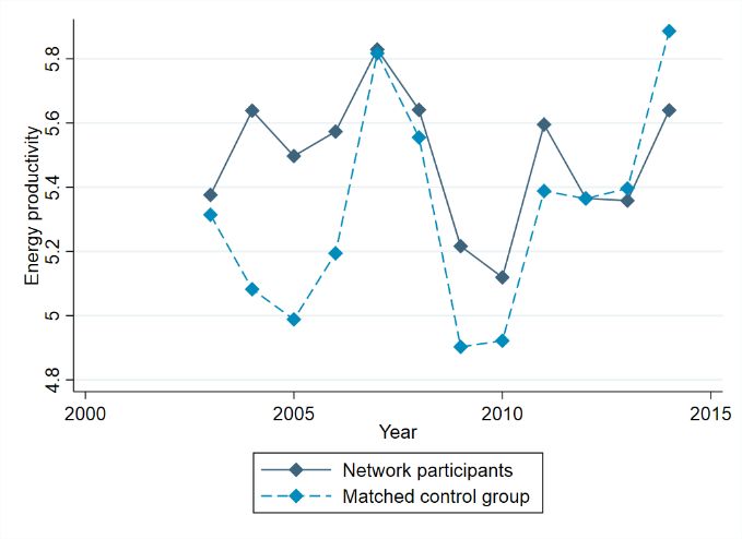
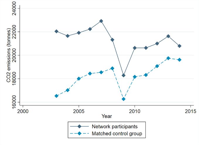
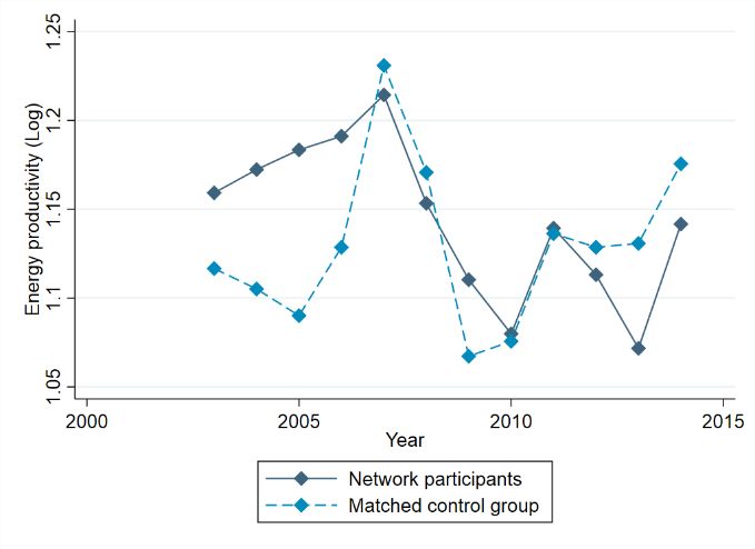
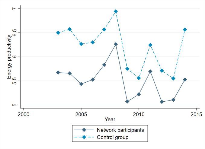
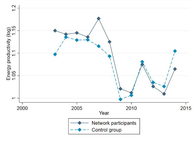
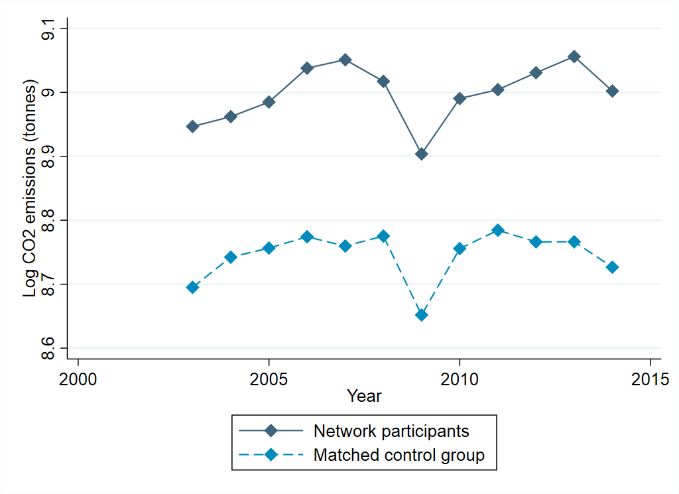
In sum, while all signs of the DiD models are in the expected direction, no robust statistically
significant effect can be found for the average network participant. The estimated treatment effects
are insignificant when energy productivity and CO2 emissions are measured in logs. The effect also
vanishes when the largest plants are excluded from the regressions. This suggests that energy
efficiency networks may have led to energy productivity improvements and CO2 savings for some
firms, but not on average.

5.1.2 Assessment of identifying assumptions

The main identifying assumption underlying ( 1 ) to ( 3 ) is that treatment and control group follow
common trends. In other words, unobserved factors affecting energy efficiency of companies that
are either part of a network or outside of a network are constant over time. Since the parallel
trends assumption of the conventional difference-in-differences estimator cannot be tested directly,
a common procedure is to look at a graph of pre-treatment trends. Figure 3 provides visual
evidence for the validity of the parallel trends assumption for the pre-treatment period (until 2008)
for the dependent variables (log) energy productivity (Panel A), as well as (log) CO2 emissions
(Panel B).19

 Figure 3: Development of energy productivity and CO2 emissions for firms in the pilot networks
 and the control group of the DiD estimator
 Panel A: Log energy productivity Panel B: Log CO2 emissions

Source: FDZ (2014b), own calculations.

In addition to a visual inspection of the pre-treatment graphs, I test for anticipation effects.20 The
idea is to test whether companies are already on an upward trajectory with respect to their energy
efficiency when they join a network. I estimate three variants of each specification shown in Table
3, with up to three pseudo-treatment dummies that indicate a treatment in the years prior to the
start of the energy efficiency networks. Of the 72 estimated pseudo-treatment effects21, only the
first lag of CO2 emissions (in levels) in the plant-level fixed effects model ( 3 ) is significant at the

19 The development of absolute energy productivity and CO2 emissions is shown in Figure A-2 in the appendix. The
parallel trends assumption seems to hold for energy productivity, but not for absolute CO2 emissions.
20 The results for the anticipation effects estimation of the plant fixed effects model ( 3 ) are shown in the appendix

(Table A-2). The results for the other models are available from the author on request.
21 For each of the four dependent variables (energy productivity, log energy productivity, CO emissions and log CO
 2 2
emissions) I estimate three different specifications (as in section 3.1), each estimated separately with one, two and three
lags.
 16

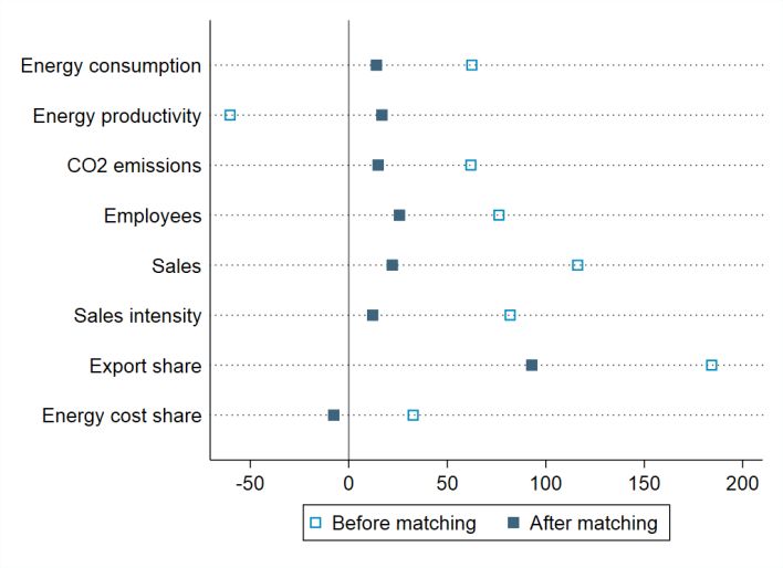
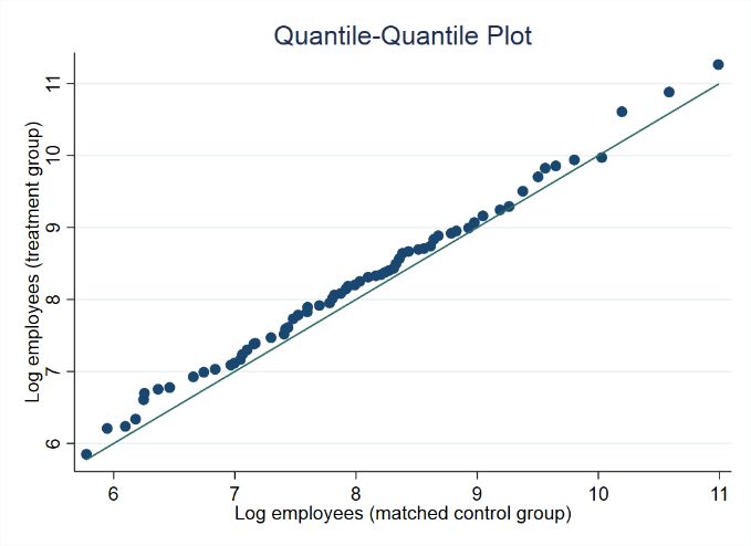
ten per cent level; all other lags are insignificant (see Table A-2 in the appendix). This adds
confidence to the validity of the common trends assumption.

A second assumption of the DiD estimator is the Stable Unit Treatment Value Assumption
(SUTVA). This assumption requires that treatment does not spill over from treated firms to
untreated firms (Imbens and Rubin, 2015). In general, it is reasonable to assume that knowledge
gained in the network meetings should not spill over to non-participating plants in the short run,
since companies do not have an interest to share the knowledge gained in energy efficiency
networks with their competitors. However, in the case that a parent company owns multiple plants,
it cannot be ruled out that non-participating installations profit from the knowledge acquired by
their peers that did participate in energy efficiency networks.22 In telephone interviews conducted
for this paper, managers of energy efficiency networks confirmed that typically all production sites
of a company participating in an EEN that are in close geographic proximity to the network also
take part in the network and are therefore identified as part of the treatment group. Additionally, in
order to rule out potential spillovers within corporations, I exclude from the control group of the
post-2015 networks those plants that belong to the same parent company as manufacturers that
took part in the pilot networks.

5.2 Conditional DiD matching estimator

5.2.1 Setup

Although the control group chosen for the difference-in-differences estimator is much more
similar to the firms participating in the pilot energy efficiency networks than the average
manufacturing firm in terms of observables, some differences between these groups remain (cf.
Table 1). In order to improve the overlap of treatment and control group, as a robustness check I
use nearest neighbour matching to identify a control group. In contrast to the previous section, for
each treated company the conditional DiD matching estimator chooses the closest match out of a
rich set of plants from the entire manufacturing sector for the estimation of treatment effects.

The nearest neighbour matching estimator constructs the counterfactual estimate for each
treatment case by selecting the nearest neighbours and setting the weights 0, 1 equal to 1/ 
for the selected neighbours, and zero for all other members of the comparison group. In the
baseline estimations, I estimate treatment effects based on one nearest neighbour matching (1:1),
and re-estimate with three nearest neighbours to demonstrate robustness of the results. To mitigate
the challenge that the energy efficiency networks start in different years (cf. appendix A.2), I only
include firms in the matching estimation that started between May 2009 and February 2011.
Consequently, there is a maximum difference of time spent in a network of 1.5 years within the
treatment group.23

Since the German manufacturing sector consists of around 43,000 firms, I have a large group of
potential nearest neighbours for each treated observation. It is therefore possible to match on
several variables without compromising too much on the matching quality. I impose the strictest

22 If different production sites of a parent company – some of which are part of an energy efficiency network, while
others are not – share the same energy manager, for example, the manager could make use of the knowledge gained in
the network for the other production sites.
23 I exclude three networks or 10 per cent of the treatment group due to this restriction.

 17