Modelling the potential impacts of the recent, unexpected increase in CFC-11 emissions on total column ozone recovery - ACP
←
→
Page content transcription
If your browser does not render page correctly, please read the page content below
Atmos. Chem. Phys., 20, 7153–7166, 2020
https://doi.org/10.5194/acp-20-7153-2020
© Author(s) 2020. This work is distributed under
the Creative Commons Attribution 4.0 License.

Modelling the potential impacts of the recent, unexpected increase
in CFC-11 emissions on total column ozone recovery
James Keeble1,2 , N. Luke Abraham1,2 , Alexander T. Archibald1,2 , Martyn P. Chipperfield3,4 , Sandip Dhomse3,4 ,
Paul T. Griffiths1,2 , and John A. Pyle1,2
1 Department  of Chemistry, University of Cambridge, Cambridge, UK
2 National Centre for Atmospheric Science (NCAS), University of Cambridge, Cambridge, UK
3 School of Earth and Environment, University of Leeds, Leeds, UK
4 National Centre for Earth Observation (NCEO), University of Leeds, Leeds, UK

Correspondence: James Keeble (james.keeble@atm.ch.cam.ac.uk)

Received: 20 August 2019 – Discussion started: 2 October 2019
Revised: 9 April 2020 – Accepted: 28 April 2020 – Published: 19 June 2020

Abstract. The temporal evolution of the abundance of long-       dicate that, if rapid action is taken to curb recently identified
lived, anthropogenic chlorofluorocarbons in the atmosphere       CFC-11 production, then no significant delay in the timing
is a major factor in determining the timing of total column      of the TCO return to the 1960–1980 mean is expected, high-
ozone (TCO) recovery. Recent observations have shown that        lighting the importance of ongoing, long-term measurement
the atmospheric mixing ratio of CFC-11 is not declining as       efforts to inform the accountability phase of the Montreal
rapidly as expected under full compliance with the Montreal      Protocol. However, if the emissions are allowed to continue
Protocol and indicate a new source of CFC-11 emissions. In       into the future and are associated with the creation of large
this study, the impact of a number of potential future CFC-      banks, then significant delays in the timing of the TCO return
11 emissions scenarios on the timing of the TCO return to        date may occur.
the 1960–1980 mean (an important milestone on the road
to recovery) is investigated using the Met Office’s Unified
Model (Hewitt et al., 2011) coupled with the United King-
dom Chemistry and Aerosol scheme (UM-UKCA). Key un-              1   Introduction
certainties related to this new CFC-11 source and their im-
pact on the timing of the TCO return date are explored, in-      The discovery of the ozone hole by Farman et al. (1985)
cluding the duration of new CFC-11 production and emis-          led quickly to the confirmation of the idea put forward by
sions; the impact of any newly created CFC-11 bank; and the      Molina and Rowland (1974) that chlorine radical species,
effects of co-production of CFC-12. Scenario-independent         the breakdown products of the chlorofluorocarbons (CFCs),
relationships are identified between cumulative CFC emis-        could deplete stratospheric ozone. In the face of the scien-
sions and the timing of the TCO return date, which can be        tific evidence, the Montreal Protocol on substances that de-
used to establish the impact of future CFC emissions path-       plete the ozone layer was agreed in 1987 and ratified in 1989.
ways on ozone recovery in the real world. It is found that,      The original controls proposed were modest, covering only
for every 200 Gg Cl ( ∼ 258 Gg CFC-11) emitted, the timing       CFCl3 (CFC-11), CF2 Cl2 (CFC-12), three further CFCs, and
of the global TCO return to 1960–1980 averaged values is         three brominated compounds (halons). However, in line with
delayed by ∼ 0.56 years. However, a marked hemispheric           the developing scientific understanding, the controls were
asymmetry in the latitudinal impacts of cumulative Cl emis-      subsequently strengthened in a series of adjustments and
sions on the timing of the TCO return date is identified, with   amendments to the Protocol. These included stronger reg-
longer delays in the Southern Hemisphere than the Northern       ulation on the phase-down schedules, the addition of many
Hemisphere for the same emission. Together, these results in-    more CFCs, CCl4 , and transitional hydrochlorofluorocarbon
                                                                 (HCFC) compounds under the London Amendment in 1990,

Published by Copernicus Publications on behalf of the European Geosciences Union.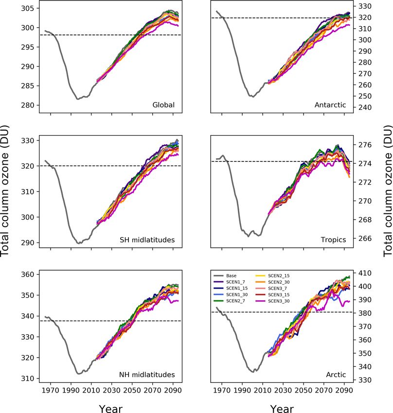
7154                                     J. Keeble et al.: Potential impacts of recent CFC-11 emissions on ozone recovery

and the inclusion of many more brominated compounds, in-         bons was also suggested by Ashfold et al. (2015) and Fang et
cluding methyl bromide under the Copenhagen Amendment            al. (2018).
of 1992. The initial replacements for the CFCs, the HCFCs,          Against this background, Montzka et al. (2018) showed
have shorter lifetimes than the CFCs (Chipperfield et al.,       that the atmospheric abundance of one of the major chlorine-
2014), and accordingly their impact on stratospheric ozone       carrying CFCs, CFC-11, is not declining as expected un-
is less. They, in turn, are being replaced by hydrofluorocar-    der full compliance with the Montreal Protocol. Using the
bons (HFCs), compounds which do not directly lead to ozone       NOAA network of ground-based observations, they demon-
depletion but some of which are strong greenhouse gases.         strated clearly that the rate of decline of CFC-11 in the atmo-
Regulations to limit the growth of many HFCs were agreed         sphere between 2015 and 2017 was about 50 % slower than
in the Kigali Amendment in 2016.                                 that observed during 2002–2012 and was also much slower
   In consequence, the atmospheric abundances of ozone-          than had been projected by WMO (2014). They inferred that
depleting chlorine and bromine species are now declining,        emissions of CFC-11 had been approximately constant at ∼
following their peaks in the late 1990s (WMO, 2018), lead-       55 Gg yr−1 between 2002 and 2012 and had then risen after
ing to the start of ozone recovery. The 2018 Scientific As-      2012 by 13 Gg yr−1 to ∼ 68 Gg yr−1 . Montzka et al. (2018)
sessment for the Montreal Protocol (WMO, 2018) reported          argued that this increase could not be explained by increased
that the Antarctic ozone hole, while continuing to occur each    release from pre-existing banks. Instead, they suggested that
year, is showing early signs of recovery (e.g. Solomon et al.,   production of CFC-11 in east Asia, which is inconsistent
2016) and that upper-stratospheric ozone has increased by        with full compliance of the Montreal Protocol, was the
up to 3 % since 2000 (e.g. LOTUS, 2019). However, there is       likely cause. Using inverse modelling, Rigby et al. (2019)
as yet no significant recovery trend in global column ozone      have since shown that the increase in CFC-11 emissions
(e.g. Ball et al., 2018; Weber et al., 2018). Furthermore,       from eastern China between 2008–2012 and 2014–2017 is ∼
because many ozone-depleting substances (ODSs) are also          7 Gg yr−1 , corresponding to approximately 40 %–60 % of the
greenhouse gases, their control has brought significant cli-     global emission increase identified by Montzka et al. (2018)
mate benefits (Velders et al., 2007, 2012; WMO, 2018). The       during that period. The increase in CFC-11 emissions af-
annual reduction in these greenhouse gas emissions is esti-      ter 2012, in conjunction with the expected decline in global
mated to be about 5 times larger than the annual emission        CFC-11 emissions which would have resulted from full com-
reduction target for the first commitment period of the Kyoto    pliance with the Montreal Protocol, has resulted in global
Protocol (WMO, 2014).                                            CFC-11 emissions being ∼ 35 Gg yr−1 greater than antici-
   The Montreal Protocol has undoubtedly been successful.        pated by the WMO (2014) A1 scenario in 2019.
Without the Protocol the abundance of ODSs would likely             The exact source of the emissions remains unknown, nor
have risen such that, for example, very large ozone de-          is it known if there is co-production of CFC-12. It is usual
pletion could have occurred in the Arctic (Chipperfield et       that the gases are produced together in an industrial plant
al., 2015). Uncontrolled growth of ODSs would also have          (e.g. Siegemund et al., 2000), with the fraction of CFC-11
severely exacerbated the impact on global warming of the         to CFC-12 production varying between 0.3 to 0.7 (UNEP,
increase in other greenhouse gases, making current climate       2018). There is currently no evidence that CFC-12 concen-
targets even more challenging to meet. However, there have       trations in the atmosphere are also declining at a slower rate
recently been questions about the completeness of the im-        than expected but some co-production of CFC-12 along with
plementation of the Protocol. The concentrations of some         CFC-11 is always expected.
short-lived anthropogenic halocarbons, which are not cov-           Compliance with the Montreal Protocol is essential for
ered by the Protocol, have increased in the atmosphere (Hos-     its continued success in reducing stratospheric Cly and ul-
saini et al., 2017; Oram et al., 2017; Fang et al. 2018), with   timately healing the ozone layer. Any non-compliance will
suggestions that they might be by-products in the produc-        inevitably prolong the period when the Antarctic ozone hole
tion of other halocarbons. Furthermore, the concentrations       will continue to occur and delay the date at which global to-
of some of the controlled ODSs have not followed pro-            tal column ozone (TCO) returns to it 1980s values, an im-
jections based on their phase-out under the Montreal Pro-        portant milestone on the road to recovery. Recent studies by
tocol. For instance, concentrations of carbon tetrachloride,     Dameris et al. (2019) and Dhomse et al. (2019) have explored
CCl4 , have not fallen as rapidly as expected based on its       a range of different future ODS loadings, enhanced above
atmospheric lifetime. A detailed reanalysis of CCl4 indi-        those expected under full compliance with the Montreal Pro-
cates that inadvertent by-product emissions from the produc-     tocol, and find substantial delays in recovery depending on
tion of chloromethanes and perchloroethylene, and fugitive       the scenario. It is essential therefore to understand the likely
emissions from the chlor-alkali process, have contributed to     impact of the current non-compliance. Here the UM-UKCA
this discrepancy (SPARC, 2016; Sherry et al., 2018; WMO,         chemistry–climate model (CCM) is used to assess the possi-
2018), and recently Lunt et al. (2018) have shown that emis-     ble implications of the change in decline of CFC-11. A num-
sions of CCl4 from east China have increased in the last         ber of possible scenarios are explored in a range of sensitivity
decade. East China as a source of other short-lived halocar-     calculations. These include emissions which cease immedi-

Atmos. Chem. Phys., 20, 7153–7166, 2020                                            https://doi.org/10.5194/acp-20-7153-2020
J. Keeble et al.: Potential impacts of recent CFC-11 emissions on ozone recovery                                         7155

ately or which persist for different periods into the future.    CH3 OOH, HCHO) alongside detailed HOx and NOx chem-
These scenarios also consider that some of the non-compliant     istry. The chemical tracers O3 , CH4 , N2 O, CFC-11, CFC-12,
production may be stored in new CFC-11 banks, for later re-      CFC-113, and HCFC-22 are all interactive with the radia-
lease, and that production of CFC-11 may be associated with      tion scheme. The halogenated source gases CFC-11, CFC-
co-production of CFC-12.                                         12, CFC-113, HCFC-22, halon-1211, halon-1301, CH3 Br,
   Until the source of the recent CFC-11 emissions is un-        CH3 Cl, CCl4 , CH2 Br2 , and CHBr3 are considered explicitly,
derstood and thoroughly quantified, model calculations can       the concentration of each prescribed at the surface as a time-
only investigate a range of possible future emissions scenar-    evolving lower boundary condition (LBC).
ios. However, models can be used to search for a relationship       The version of UM-UKCA used in this study is an
between the amount of chlorine emitted into the atmosphere       atmosphere-only configuration, with each simulation using
and the timing of TCO return dates. Here results from both       the same prescribed sea surface temperatures (SSTs) and
the UM-UKCA CCM and the TOMCAT chemistry transport               sea ice fields taken from a parent coupled atmosphere–ocean
model (CTM; recently used to study the impact of increased       HadGEM2-ES integration. The configuration of the model
CFC-11 emissions on the behaviour of the Antarctic ozone         used for this study includes the effects of the 11-year solar
hole; Dhomse et al., 2019) are used to investigate the rela-     cycle in both the radiation and photolysis schemes. The top-
tionship between increased emissions and enhanced ozone          of-the-atmosphere solar flux follows historical observations
depletion. Identification of a robust relationship would allow   from 1960 to 2009, after which a repeating solar cycle is im-
us to develop a scenario-independent understanding of the        posed which is an amplitude equivalent to the observed cycle
impact of uncontrolled CFC emissions on the TCO return           23 (as detailed in Bednarz et al., 2016). Further information
date.                                                            on the model configuration used for this study is provided in
   In Sect. 2 the UM-UKCA and CFC scenarios used in this         Keeble et al. (2018). Except for CFC-11 and CFC-12 LBCs,
study are discussed in detail. Section 3 assesses the impact     all other chemical forcings in the simulations follow the ex-
of these CFC emissions scenarios on stratospheric chlorine       perimental design of the WCRP/SPARC Chemistry Climate
loading before the impacts on the TCO return date are ex-        Model Initiative (CCMI) REF-C2 experiment (Eyring et al.,
amined in Sect. 4. Section 5 investigates the relationship be-   2013), which adopts the RCP6.0 scenario for future green-
tween cumulative CFC emissions and ozone depletion, using        house gas (GHG) and ODS emissions. A baseline experiment
both the CCM and CTM. Finally, further discussion of the         (BASE) performed using CFC-11 and CFC-12 LBCs pro-
results and a summary of our conclusions are provided in         vided by the WMO (2014) A1 scenario was run from 1960
Sect. 6.                                                         to 2099. A further nine simulations were performed, running
                                                                 from 2012 to 2099, using a range of CFC-11 and CFC-12
                                                                 LBCs, which were designed to cover a large but plausible
2   Model configuration and simulations                          range of potential future CFC emissions scenarios given the
                                                                 associated uncertainties.
To explore the impacts of potential future CFC-11 emission
scenarios on the TCO return date, a total of 10 transient        2.1   CFC-11 scenarios
simulations were performed using the UM-UKCA model,
which consists of version 7.3 of the HadGEM3-A configura-        There are a number of important details associated with the
tion of the Met Office’s Unified Model (Hewitt et al., 2011)     recently reported CFC-11 emissions from East Asia which
coupled with the United Kingdom Chemistry and Aerosol            are poorly understood. A key factor is whether the identi-
scheme. This configuration of the model has a horizontal         fied CFC-11 emissions arise from emissive or non-emissive
resolution of 2.5◦ latitude ×3.75◦ longitude, and 60 verti-      uses. If they arise from a totally emissive use, then the ob-
cal levels following a hybrid sigma-geometric height coor-       served CFC-11 changes represent the total new CFC-11 pro-
dinate, extending from the surface to a model top at 84 km.      duction, with this new source of CFC-11 being released into
The chemical scheme is an expansion of the scheme pre-           the atmosphere during either production or use. Conversely,
sented in Morgenstern et al. (2009) in which halogen source      if they arise from a non-emissive use (e.g. foam insulation),
gases are considered explicitly and the effects of the solar     then the observed changes to CFC-11 represent only a frac-
cycle are considered as described in Bednarz et al. (2016).      tion of the total production, with a large component entering
It includes 45 chemical species, 118 bimolecular reactions,      a new bank. In order to address this, two scenario types were
17 termolecular reactions, 41 photolysis, and 5 heteroge-        created, which reflect the new CFC-11 production which is in
neous reactions occurring on the surfaces of polar strato-       addition to that implied in the WMO (2014) A1 scenario. In
spheric clouds and sulfate aerosols. This chemistry scheme       SCEN1, which represents the emissive use scenario, constant
provides a detailed treatment of stratospheric chemistry in-     emissions of 35 Gg CFC-11 yr−1 (∼ 27 Gg Cl yr−1 ) were as-
cluding the Ox , ClOx , BrOx , HOx , and NOx catalytic cycles    sumed while in SCEN2 total production was assumed to
and a simplified tropospheric scheme including the oxidation     be 90 Gg CFC-11 yr−1 (∼ 70 Gg Cl yr−1 ), with 15 Gg CFC-
of a limited number of organic species (CH4 , CO, CH3 O2 ,       11 yr−1 of this total directly emitted into the atmosphere,

https://doi.org/10.5194/acp-20-7153-2020                                         Atmos. Chem. Phys., 20, 7153–7166, 2020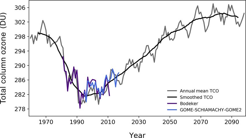
7156 J. Keeble et al.: Potential impacts of recent CFC-11 emissions on ozone recovery
while the remaining 75 Gg CFC-11 yr−1 entered a bank with
an assumed release fraction of 3.5 % yr−1 . The SCEN2 sce-
nario is designed to give an additional emission increment of
∼ 35 Gg CFC-11 yr−1 in 2019, similar to the emissions value
used in SCEN1 and consistent with the CFC-11 emissions
increment, in addition to that expected assuming only re-
lease from known banks, identified by Montzka et al. (2018.)
We emphasis that the 35 Gg CFC-11 yr−1 and 90 Gg CFC-
11 yr−1 values represent the extra emissions or production
increment assumed in addition to those of the WMO (2014)
A1 scenario.
A second key factor is the duration of the illegal produc-
tion. In order to address this question, three sets of simula-
tion were performed for both SCEN1 and SCEN2, in which
uncontrolled production either stopped in 2019 or continued
into the future until 2027 or 2042, giving total emissions
periods of 7, 15, or 30 years, respectively. All simulations
assume that uncontrolled production and emission began in
2012. Simulations are named such that the scenario name
is followed by the emission period, separated by an under-
score (i.e. SCEN1_15 uses SCEN1 emissions from 2012 for
15 years).
A third consideration is the potential co-production of
CFC-12. While there is no evidence currently that CFC-12
concentrations in the atmosphere are declining at a slower
rate than expected (Montzka et al., 2018), CFC-12 is com-
monly co-produced alongside CFC-11 at a ratio of 30:70 ei-
ther way (TEAP, 2019). Accordingly, an additional scenario
(SCEN3) was developed in which 90 Gg yr−1 of both CFC-
11 and CFC-12 is produced, i.e. a ratio of 50 : 50, towards
the middle of the expected range. The same assumptions
are made about the relative fraction entering the bank and
the subsequent bank release rate as for SCEN2. SCEN3 was
performed for the three different emissions periods used by
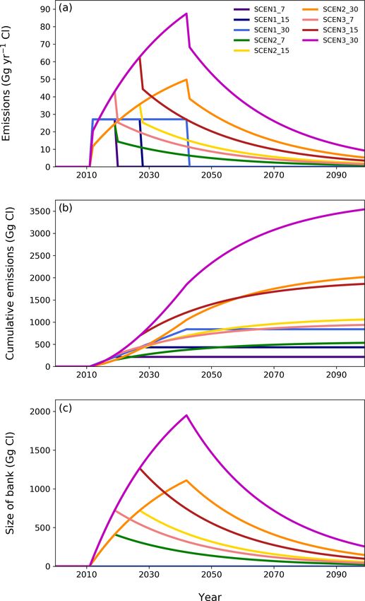
SCEN1 and SCEN2, and simulations follow the same nam- Figure 1. (a) Additional emissions (in Gg Cl yr−1 ) assumed for
ing convention. As we consider both CFC-11 and CFC-12, each of the SCEN simulations on top of those already assumed by
all future emission or production values will be given in gi- the WMO (2014) A1 scenario. For all scenarios, the additional, un-
gagrams of chlorine with 1 Gg CFC-11 equal to ∼ 0.77 Gg Cl controlled source of emissions is assumed to start in 2012. (b) Cu-
and 1 Gg CFC-12 equal to ∼ 0.59 Gg Cl. mulative additional emissions for each of the SCEN simulations.
The emissions for these various scenarios are shown (in (c) The size of the newly created bank for the SCEN2 and SCEN3
scenarios.
Gg Cl) in Fig. 1a, while Fig. 1b shows the cumulative emis-
sions and Fig. 1c shows the size of the newly created bank.
The SCEN3 scenarios include both CFC-11 and CFC-12,
both scaled to gigagrams of chlorine and summed. sions. After that point, all emissions emanate from the newly
Figure 1a highlights that the SCEN1 scenario emissions created bank. The maximum size of emissions is dictated
stop at the end of the assumed production, while for the by the duration of production. For comparison, Daniel et
SCEN2 and SCEN3 scenarios emissions continue through- al. (2007) estimate that peak CFC-11 production, before the
out the 21st century long after the cessation of production adoption of the Montreal Protocol, reached ∼ 300 Gg Cl yr−1
due to the newly created bank. For SCEN2 and SCEN3 the in 1986–1987. For SCEN1 scenarios, cumulative emissions
shapes of the emissions curves are controlled by the combi- increase only during the period of assumed production; there
nation of direct emission and newly created bank. While pro- is no newly created bank. For the SCEN2 and SCEN3 sce-
duction continues, the yearly direct emissions remain con- narios cumulative emissions grow most rapidly during the
stant, but the bank grows, leading to larger total emissions period when direct emissions occur, but they continue to in-
per year. At the moment production stops the direct emis- crease throughout the 21st century due to emissions from the
sions also stop, resulting in a marked step down in the emis- bank. The size of the newly created bank is dependent on
Atmos. Chem. Phys., 20, 7153–7166, 2020 https://doi.org/10.5194/acp-20-7153-2020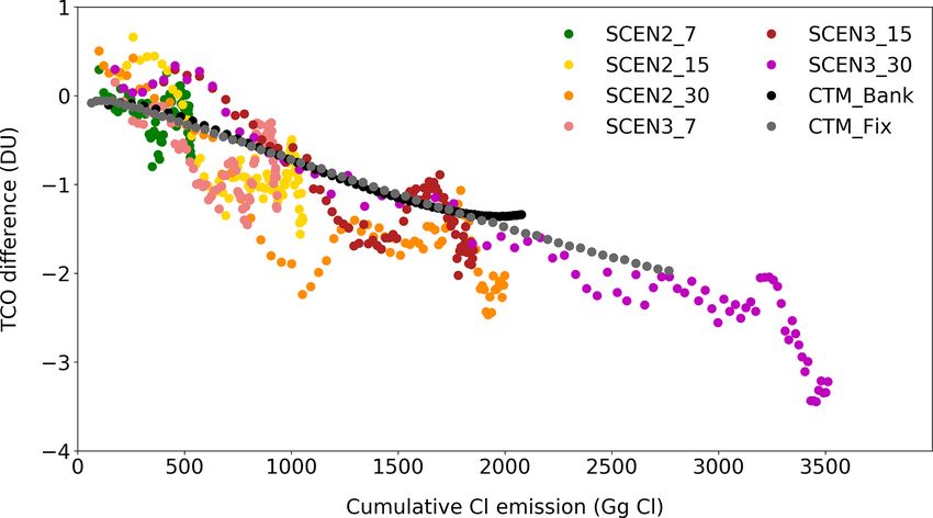
J. Keeble et al.: Potential impacts of recent CFC-11 emissions on ozone recovery 7157
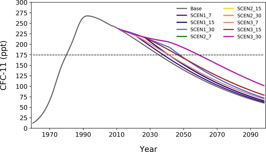
Figure 2. Prescribed global mean, annual mean surface lower Figure 3. Modelled annual mean 40 km inorganic chlorine (Cly )
boundary mixing ratio of CFC-11 used for the BASE and SCEN mixing ratios, averaged from 10◦ S–10◦ N, for the BASE and SCEN
simulations. The dashed line represents the 1980 CFC-11 surface simulations. The dashed line represents the 1980 Cly mixing ratio
mixing ratio in the BASE simulation. Note that the SCEN2 and at 40 km in the BASE simulation, used as the value for calculating
SCEN3 simulations have the same CFC-11 lower boundary con- the Cly return date.
ditions.
lays in the stratospheric chlorine return date are modelled in
the duration of production and the release rate from the bank the SCEN2 simulations, which assume a large bank is also
(Fig. 1c), which was assumed to be 3.5 % yr−1 . being produced alongside the direct atmospheric emissions
As discussed above, the UM-UKCA uses prescribed LBC (see Fig. 1). In the SCEN2_7 scenario, which assumes CFC-
mixing ratios of CFCs. As a result, each of the emissions 11 production stops in 2019, the stratospheric Cly return date
scenarios described above was converted into LBC mixing is delayed by 2 years, and for SCEN2_30, which assumes
ratios using a simplified box model which uses only the emis- CFC-11 production continues until 2042, the stratospheric
sions flux and a CFC-11 lifetime of 55 years. This model Cly return date is delayed by 8 years. The delays highlight
reproduces to within good agreement the observed 1994– the potential importance for ozone depletion of any bank pro-
2017 CFC-11 surface mixing ratio when initialized with the duced and its subsequent emission into the atmosphere. The
1994 values and using the emission estimates of Montzka et delay in the stratospheric Cly return date is larger still if co-
al. (2018). The time variation of CFC-11 at the surface is production of CFC-12 is considered, with the stratospheric
shown in Fig. 2 for the different scenarios. Cly return date being delayed by 14 years in the SCEN3_30
scenario considered here.
3 Stratospheric chlorine
4 Modelled total column ozone response
Increases in stratospheric chlorine will lead to ozone deple-
tion, and so uncontrolled production of CFCs could obvi- Figure 4 shows the annual mean TCO data from the BASE
ously pose a serious threat to the continued success of the simulation (grey line) from 1960 to 2100, averaged over
Montreal Protocol. Modelled 40 km stratospheric inorganic 60◦ S–60◦ N. Consistent with previous studies, TCO values
chlorine (Cly ) mixing ratios, averaged from 10◦ S–10◦ N, are decrease sharply from 1980 to the late 1990s as a result of in-
shown in Fig. 3, and stratospheric Cly return dates (the date creasing stratospheric chlorine loadings, before gradually in-
at which Cly mixing ratios, averaged from 10◦ S–10◦ N at creasing throughout the 21st century. Superimposed on these
40 km, return to the BASE 1980 value) are given in Table 1. long-term trends is an 11-year oscillation resulting from the
We chose the 10◦ S–10◦ N latitude range for calculating Cly solar cycle. Observed annual mean TCO values from ver-
return dates as this is within the tropical pipe in which air is sion 2.8 of the Bodeker Scientific total column ozone dataset
predominantly moved vertically with limited horizontal mix- (Bodeker et al., 2005) are shown in purple. There is gener-
ing (e.g. Waugh, 1996; Neu and Plumb, 1999), a necessary ally good agreement between modelled TCO values and the
consideration as Cly varies latitudinally with age of air. In the Bodeker dataset; decadal total column ozone changes, the
BASE simulation, the stratospheric Cly mixing ratio is pro- response of column ozone to the solar cycle, and the mag-
jected to return to its 1980 value by 2058. Only small differ- nitude of interannual variability are all well captured by the
ences in the stratospheric Cly return date are modelled for the model throughout the time period during which the observa-
SCEN1 simulations, with a maximum delay of 3 years occur- tions and model data overlap.
ring in the SCEN1_30 simulation, which assumes the longest As discussed by Keeble et al. (2018; following WMO,
duration of additional CFC-11 emissions. However, large de- 2007; Chipperfield et al., 2017), three stages of ozone recov-
https://doi.org/10.5194/acp-20-7153-2020 Atmos. Chem. Phys., 20, 7153–7166, 2020
7158                                         J. Keeble et al.: Potential impacts of recent CFC-11 emissions on ozone recovery

Table 1. Cly return date (defined as the date at which Cly mixing ratios, averaged from 10◦ S–10◦ N at 40 km, return to the BASE simulation
1980 value) and the date TCO returns to the 1960–1980 mean in the BASE and SCEN simulations. Uncertainty estimates for the TCO return
date in the BASE simulation are provided by a separate five-member ensemble, as described in the text. TCO return to the 1960–1980 mean
occurs after 2080 for the latitude range 90–60◦ S, and so no uncertainty estimate can be provided for this latitude band, denoted by “±?” in
the table.

                      Cly return date                  Date of total column ozone (TCO) return to 1960–1980 mean.
                         10◦ S–10◦ N     60◦ S–60◦     90◦ S–60◦ S    60◦ S–30◦ S     30◦ S–30◦ N     30◦ N–60◦ N     60◦ N–90◦ N
        BASE                    2058      2054 ± 2       2084 ± ?        2065 ± 1        2057 ± 3         2047 ± 2        2048 ± 3
        SCEN1_7                 2059         2055            2078           2061            2060             2050            2050
        SCEN1_15                2057         2055            2082           2064            2062             2050            2052
        SCEN1_30                2061         2057            2088           2068            2063             2049            2048
        SCEN2_7                 2060         2055            2084           2065            2060             2047            2049
        SCEN2_15                2062         2058            2093           2071            2065             2051            2052
        SCEN2_30                2066         2061            2095           2071            2069             2052            2057
        SCEN3_7                 2061         2058            2081           2064            2063             2052            2054
        SCEN3_15                2064         2058        No return          2068            2066             2053            2053
        SCEN3_30                2073         2064        No return          2074            2081             2052            2052

                                                                        tween the timing of the global TCO return to these three
                                                                        values. However, differences do occur in regions with high
                                                                        interannual variability (e.g. the Arctic).
                                                                           As discussed in previous studies (e.g. Salby et al., 2011;
                                                                        Ball et al., 2018), the identification of total column ozone
                                                                        recovery is complicated by the effects of interannual vari-
                                                                        ability. To mitigate these impacts, the effects of natural pro-
                                                                        cesses (such as volcanic eruptions, the quasi-biennial oscilla-
                                                                        tion, El Niño–Southern Oscillation, and the solar cycle) can
                                                                        be removed from the data using statistical techniques (such
                                                                        as multiple linear regression – e.g. Staehelin et al., 2001;
                                                                        WMO, 2007; the Time series Additive Model – Scinocca et
Figure 4. Modelled annual mean TCO values (in DU), averaged             al., 2010), or the data can be smoothed by averaging across
from 60◦ S to 60◦ N, for the BASE (grey line) and smoothed data         multiple years (e.g. Dhomse et al., 2018). Following Dhomse
(black line), using an 11-point boxcar smoothing to reduce the ef-      et al. (2018), annual mean UM-UKCA data is smoothed us-
fects of both interannual variability and the solar cycle (follow-      ing an 11-point boxcar smoothing to reduce both the effects
ing Dhomse et al., 2018). Also shown are TCO values, averaged           of short-term variability and the signature of the 11-year so-
over 60◦ S–60◦ N, from v2.8 of the Bodeker dataset (purple line;        lar cycle. The smoothed data are shown on Fig. 4 as the black
Bodeker et al., 2005) and v3 of the GOME/SCIAMACHY/GOME2                line. For the analysis in subsequent sections, all data from
Merged Total Ozone dataset (blue line; Weber et al., 2011).             the BASE and SCEN simulations are smoothed using this
                                                                        method.
                                                                           Ideally, to provide uncertainty estimates for our various in-
ery can be identified: (i) a slowed rate of decline and the date        tegrations, a multi-member ensemble would be run for the
of minimum column ozone, (ii) the identification of signifi-            BASE and each SCEN calculation. However, in order to
cant positive trends, and (iii) a return to historic values. Here,      explore the largest possible range of future CFC-11 emis-
we focus on the impact of uncontrolled CFC-11 emissions                 sions scenarios, only one integration was performed for each
on the last of these metrics: return to historic values, with           scenario. Instead, data from a separate five-member ensem-
the historic baseline value defined as the total column ozone           ble of 1980–2080 transient simulations (see Bednarz et al.,
average from 1960 to 1980. This definition of the baseline              2016) is used to provide a rough estimate of the uncertainty
period was chosen to avoid any sensitivity of the TCO re-               range of return dates. These simulations used the same model
turn date to the choice of any individual year (which may be            configuration as used for our BASE and SCEN calculations
anomalously high or low). In actuality, global (60◦ S–60◦ N)            but were forced with the older WMO (2011) CFC-11 and
TCO averaged from 1960–1980 in the BASE simulation is                   CFC-12 LBCs. Uncertainty estimates were estimated sim-
298.1 DU, and the values for 1960 and 1980 are 297.5 and                ply by identifying the ensemble member with the largest dif-
298.0 DU, respectively, and so there is little difference be-           ference in return date from the ensemble mean and defining

Atmos. Chem. Phys., 20, 7153–7166, 2020                                                    https://doi.org/10.5194/acp-20-7153-2020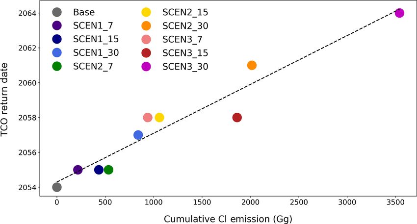
J. Keeble et al.: Potential impacts of recent CFC-11 emissions on ozone recovery                                           7159

this difference as the uncertainty range (e.g. for five ensem-   created bank, is modest with no delay modelled, except for
ble members where the return dates might be 2061, 2062,          SCEN1_30, which returns to the 1960–1980 average in 2088.
2060, 2061, and 2066, the mean return date would be 2062         In contrast, large delays are modelled for both the SCEN2_15
and the largest deviation is 2066, so the uncertainty estimate   and SCEN2_30 simulations, which have projected return
would be ±4 years). This provides an approximate indication      dates of 2093 and 2095, respectively. If co-production of
of uncertainty for all latitude ranges considered here, except   CFC-12 is considered, SCEN3_15 and SCEN3_30 suggest
for the latitude range 90◦ S–60◦ S, where TCO return to the      that 11-year averaged TCO values will not return to the
1960–1980 mean occurred after 2080 and so lies outside the       1960–1980 baseline period by the end of the 21st century.
range of the ensemble.                                              In the SH midlatitudes (60–30◦ S), delays in the return date
   For the BASE integration under the WMO (2014) sce-            are modelled for a number of SCEN simulations. If produc-
nario, a global (60◦ S–60◦ N) TCO return date of 2054 ±          tion stops in 2019, there is essentially no delay, while scenar-
2 years was calculated, with the return dates for other lat-     ios with higher emissions or longer duration lead to delays of
itudes shown in Table 1. In the next section, the impact of      between 6 (SCEN2) and 9 years (SCEN3_30, which includes
CFC-11 and CFC-12 emissions from the different SCEN sce-         co-production of CFC-12).
narios on these return dates is assessed.                           While most SCEN simulations project a delay in the re-
                                                                 turn of Antarctic and SH midlatitude annual mean TCO to
4.1   Global total column ozone                                  the 1960–1980 mean, SCEN1_7, SCEN1_15, and SCEN3_7
                                                                 all have earlier return dates than the BASE simulation. In
Figure 5 shows smoothed TCO values for the BASE and              the case of SCEN1_7 these changes in the SH midlatitudes
SCEN simulations, averaged from 60◦ S–60◦ N. All simula-         are outside the model range calculated from the Bednarz et
tions show a return to the baseline period of the 1960–1980      al. (2016) five-member ensemble, occurring 4 years earlier
average between 2054 and 2064 (return dates provided in Ta-      than in the BASE simulation. This may be because the un-
ble 1). The BASE simulation, which adopts the WMO (2014)         certainty estimates calculated here from the five-member en-
LBC for ODSs and as such assumes the lowest anthropogenic        semble do not fully capture the true system uncertainty or
Cly emissions, returns to the 1960–1980 mean the earliest,       that atmospheric chemistry–climate feedbacks may result in
in 2054, as discussed above. The impact of the additional        increased TCO values in some locations despite increased
CFC-11 and CFC-12 production scenarios investigated here         stratospheric ODS values. For example, Keeble et al. (2014)
is to delay the return date. For SCEN1_7 and SCEN1_15,           show modelled wintertime TCO increases in the northern
the delay is small and within the range of return dates cal-     midlatitudes resulting from increased polar ozone depletion
culated from the five-member ensemble. Only SCEN1_30 of          and associated changes in the lower branch of the Brewer–
the SCEN1 scenarios shows a significant delay in return date     Dobson circulation (BDC).
of 3 years. In contrast, for the SCEN2 simulations, which as-       The observed ozone loss in the tropics has been small and,
sume the creation of a new bank and subsequent emissions         furthermore, future changes in the tropics are driven both by
of CFC-11 from that bank, a substantial delay in the return      reductions in the stratospheric abundance of halogens, which
date of global TCO is modelled in both the SCEN2_15 and          tend to increase ozone, and the strengthening of the Brewer–
SCEN2_30 simulations (4 and 7 years, respectively). Only in      Dobson circulation, which tends to decrease column ozone
the case that the assumed production of 90 Gg yr−1 stops this    (e.g. Oman et al., 2010; Eyring et al., 2013; Meul et al.,
year (2019) is no significant delay in the return of TCO val-    2014; Keeble et al., 2017; Chiodo et al., 2018). Here, trop-
ues to the baseline period modelled. The SCEN3 scenarios,        ical (30◦ S–30◦ N) TCO values are projected to return to the
which assume the co-production of CFC-12 alongside CFC-          1960–1980 mean by 2057 in the BASE simulation, and all
11, all show larger delays in the return date, with this being   SCEN simulations show significant delays to this return date
10 years for SCEN3_30.                                           except for SCEN1_7 and SCEN2_7 (i.e. those simulations
                                                                 which assume that uncontrolled production of CFC-11 stops
4.2   Regional total column ozone                                in 2019 and there is no co-production of CFC-12). While
                                                                 TCO values are projected to return to the 1960–1980 average
Regional TCO projections for the BASE and SCEN simu-             for the broad definition of the tropics used here, if a narrower
lations are also shown in Fig. 5, from the Antarctic to the      definition is used (e.g. 5◦ S–5◦ N), TCO values do not return
Arctic, and TCO return dates for each region are given in Ta-    to the 1960–1980 average at any point in the 21st century.
ble 1. Annual mean TCO values over Antarctica (90–60◦ S)         This is consistent with the impacts on lower-stratospheric
return to the 1960–1980 average by 2084 in the BASE simu-        ozone of the increased speed of the BDC resulting from an-
lation, 30 years after the global (60◦ S–60◦ N) TCO average      thropogenic GHG changes (e.g. Oman et al., 2010; Eyring et
is expected to return. Substantial further delays in the date    al., 2013; Meul et al., 2016; Keeble et al., 2017).
at which Antarctic TCO returns to the 1960–1980 mean are            In the NH midlatitudes (30◦ N–60◦ N), TCO under the
modelled for a number of the SCEN simulations. Again, the        BASE projection is modelled to return in 2047, considerably
impact of the SCEN1 scenarios, which assumes no newly            earlier than the SH midlatitudes. As at other latitudes, a sig-

https://doi.org/10.5194/acp-20-7153-2020                                          Atmos. Chem. Phys., 20, 7153–7166, 2020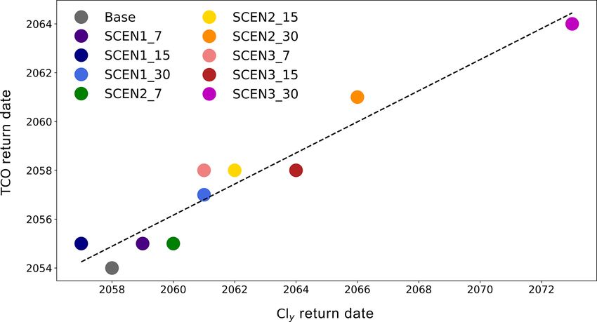
7160                                       J. Keeble et al.: Potential impacts of recent CFC-11 emissions on ozone recovery

Figure 5. Smoothed TCO (in DU) for the BASE and SCEN simulations, for the global (60◦ S–60◦ N) and regional column values. Dashed
line denotes the 1960–1980 baseline period, used as the value for calculating the TCO return date.

nificant delay in the return date is modelled in the majority       5   Identifying scenario-independent relationships
of SCEN simulations.                                                    between CFC emissions and TCO return to the
   In the Arctic (60◦ N–90◦ N), annual mean TCO values are              1960–1980 mean
projected to return to the 1960–1980 mean in the BASE sim-
ulation in 2048, again substantially earlier than the Antarc-
tic return date. While significant delays for Arctic ozone are      While the SCEN simulations used in this study were de-
modelled in the majority of SCEN simulations, unlike at             signed to cover a broad range of potential future CFC-11 pro-
other latitude ranges, the latest return dates are not associated   duction scenarios, it is unlikely that future CFC-11 emissions
with the SCEN3 simulations, which assume co-production of           will follow any of the scenarios described here. Therefore,
CFC-12. Instead, the latest return date of 2057 occurs in the       we aim here to identify scenario-independent relationships
SCEN2_30 simulations. We ascribe this to the very high dy-          between future CFC emissions pathways and the impact on
namical variability of the Arctic polar vortex, its subsequent      TCO. For example, Dhomse et al. (2018) found relationships
impact on total column ozone, and the large uncertainties in        between the chlorine return date and a number of indica-
defining a return date in this region. Bednarz et al. (2016),       tors of ozone recovery for a range of models (see, e.g., their
also using the UM-UKCA, showed that, although springtime            Fig. 8). In this study this relationship is further explored by
Arctic ozone was projected to return to 1980 values by the          linking TCO differences to emissions. Three emerging rela-
late 2030s, episodes of dynamically-driven very low ozone           tionships are explored in the following sections: (i) the timing
could be found well into the second half of this century, con-      of the global TCO return date as a function of Cly return date;
sistent with our annual mean results presented here.                (ii) the magnitude of annual mean TCO depletion in a year as
                                                                    a function of the cumulative CFC emissions up to that year;

Atmos. Chem. Phys., 20, 7153–7166, 2020                                               https://doi.org/10.5194/acp-20-7153-2020
J. Keeble et al.: Potential impacts of recent CFC-11 emissions on ozone recovery 7161
Figure 6. TCO return date (defined as the date at which 60◦ S– Figure 7. Annual mean TCO difference (in DU) for the UM-UKCA
60◦ N averaged TCO values return to the 1960–1980 average) for SCEN2 and SCEN3 simulations with respect to the BASE simula-
the BASE and SCEN simulations versus Cly return date (defined as tion, averaged over 60◦ S–60◦ N vs. cumulative emissions (Gg Cl)
the date at which Cly mixing ratios at 40 km, averaged from 10◦ S– from 2012 to that year. Grey and black points show the same, but are
10◦ N, return to the 1980 BASE value). The dashed line gives the for the CTM_Fix and CTM_Bank simulations performed with the
linear fit through the points. TOMCAT CTM. For these simulations, TCO differences are cal-
culated with respect to the CTM_C baseline simulation. TOMCAT
simulations described in Dhomse et al. (2019).
and (iii) the TCO return date as a function of the cumulative
additional CFC emissions by the end of the simulation.
5.1 Cly return date vs. TCO return date 5.2 TCO depletion vs. cumulative emissions
The future evolution of stratospheric ozone mixing ra- In order to explore the magnitude of annual mean TCO de-
tios closely follows the evolution of stratospheric Cly (e.g. pletion in any year as a function of the cumulative Cl emis-
WMO, 2018). Dhomse et al. (2018) found correlations be- sions up to that year, results from the UM-UKCA SCEN
tween modelled return dates of stratospheric chlorine and simulations are supplemented by simulations performed with
ozone recovery dates for Antarctic and Arctic spring across the TOMCAT CTM (Chipperfield et al., 2017). Both models
a range of CCMI models. A similar relationship between the have full stratospheric chemistry schemes but are indepen-
timing of a Cly return to 1980 values and the timing of the dent of one another. The control CTM simulation (CTM_C)
global TCO return to the 1960–1980 mean is identified in the was performed until 2080 with repeating year 2000 meteorol-
SCEN simulations performed as part of this study, shown in ogy and time-dependent future source gas surface mixing ra-
Fig. 6. As discussed above, the Cly return date is defined as tios. Two further simulations (described in detail in Dhomse
the date at which Cly mixing ratios at 40 km, averaged from et al., 2019) were performed with additional future CFC-11
10◦ S to 10◦ N, return to their 1980s value. The relationship emissions (i) at constant 67 Gg yr−1 (CTM_Fix) and (ii) in-
between the global TCO return date and the Cly return date cluding the simulation of a bank and production decreasing
is robust, with an r 2 of 0.92, and indicates that for every to zero over 10 years (CTM_Bank). Note that simulation
year Cly return is delayed, the TCO return date is delayed CTM_Bank gives larger emissions than CFM_Fix until about
by 0.64 years (given by the gradient of the linear fit through the year 2040.
the points). The Cly return date itself is strongly linked to Figure 7 shows the cumulative additional Cl emissions for
the assumed emissions. A robust linear relationship, with an both the UM-UKCA and TOMCAT models plotted against
r 2 value of 0.96, was identified between the total cumulative the additional TCO depletion driven by the increased emis-
additional Cl emissions and the delay in Cly return date. This sions compared with a base integration, averaged over 60◦ S–
relationship indicates that, for every additional 200 Gg of Cl 60◦ N. UM-UKCA values are calculated as the difference be-
(258 Gg CFC-11 equivalent) emitted by 2099 above those tween each SCEN simulation with respect to the BASE sim-
implied in the WMO (2014) scenario, the Cly return date is ulation, while TOMCAT values are calculated as CTM_Fix–
delayed by 0.86 years. It should be noted that the Cly return CTM_C and CTM_Bank–CTM_C. For both models, all
date occurs ∼ 5 years later on average than the global TCO available years from each scenario are plotted, with each
return date in the BASE and SCEN simulations (see Table 1), point representing a single year and showing the TCO differ-
indicating that even after the time TCO values have returned ence between the scenario and base simulation for that year
to the 1960–1980 average, stratospheric chlorine mixing ra- plotted against the cumulative Cl emissions reached by that
tios remain elevated above the 1980 value. year.
The estimated TCO depletion from both UM-UKCA and
CTM simulations follows a reasonably compact, linear rela-
https://doi.org/10.5194/acp-20-7153-2020 Atmos. Chem. Phys., 20, 7153–7166, 20207162 J. Keeble et al.: Potential impacts of recent CFC-11 emissions on ozone recovery
tionship with cumulative emissions. The CTM simulations
use identical meteorology, without any chemistry–climate
feedbacks, and so a comparison of two simulations gives a
direct measure of the chemical ozone impact of the additional
emissions. In contrast, UM-UKCA generates a consistent
time-varying meteorology for each of the SCEN simulations
and so includes both a forced response and internally gener-
ated natural variability. Despite this difference, the modelled
relationship between cumulative emissions and global ozone
depletion is remarkably similar for the two models: a total
emission of 3500 Gg (Cl) gives a near-global mean ozone
decrease of between 2.5 and 3 DU. The agreement between
the two models provides confidence in the diagnosed chem- Figure 8. TCO return date (defined as the date at which TCO values
ical impact of the CFC-11 emissions and shows a means by return to the BASE 1960–1980 average) for the BASE and SCEN
which results from different model simulations, with differ- simulations vs. cumulative additional emissions (Gg Cl) from 2012
to the end of the simulation. The dashed line gives the linear fit
ent CFC-11 emissions scenarios, can be compared. Further,
through the points.
it allows an estimate to be made of the impact of any given
CFC-11 emission scenario on TCO depletion, which can in
turn be applied to the real-world future emissions of CFC-11,
which remain uncertain.
In CTM run CFC_Bank the maximum CFC-11 emissions
by 2080 are around 2700 Gg CFC-11. By this stage a signif-
icant part of the large initial pulse of emissions (see Dhomse
et al., 2019) would have been removed from the atmosphere
(consistent with its ∼ 55-year lifetime) so that the CTM line
deviates from the simple linear fit (black line Fig. 7). This
is also true for the SCEN simulations performed with UM-
UKCA, although the effects are small compared to the dy-
namically driven variability. The SCEN1 simulations are not
shown in Fig. 7 as their cumulative emissions stop increas-
Figure 9. Delay in TCO return date (in years) per 200 Gg Cl emis-
ing when the direct emissions stop (see Fig. 1), and so for a
sions for 10◦ latitude bins. Uncertainty bars represent the standard
large period of the simulations the differences are dominated
error of the estimate (calculation method provided in text). No val-
by variability. ues are given for 90–80◦ S, 80–70◦ S, and 10◦ S–0◦ N as TCO in
these latitude bands does not return to the 1960–1980 mean by the
5.3 TCO return date vs. total cumulative emissions end of the model simulations.
Figure 8 shows the relationship between the total cumula-
Large delays (∼ 1.6 years per 200 Gg Cl) are modelled in
tive additional Cl emissions, in gigagrams, and projected the
the Antarctic, where heterogeneous processing of chlorine
global TCO return date in the BASE and SCEN simulations.
reservoirs on polar stratospheric cloud (PSC) surfaces allows
These values represent the additional Cl emissions assumed
for large ozone depletion even for relatively small chlorine
for each scenario in addition to the WMO (2014) A1 sce-
concentrations. On annual mean timescales these low val-
nario. A robust (r 2 = 0.93) linear relationship is found, indi-
ues mix into the Southern Hemisphere midlatitudes, result-
cating that for every extra 200 Gg of Cl emitted, the global
ing in larger delays to the return date there (0.5–0.8 years
TCO return to the 1960–1980 mean is delayed by 0.56 years.
per 200 Gg Cl) than in the Northern Hemisphere midlatitudes
Repeating this analysis for 10◦ latitude bins gives the latitu-
and Arctic (0.1–0.5 years per 200 Gg Cl), where the effects of
dinal dependence of the impacts of cumulative Cl emissions
PSC processing are less pronounced due to the higher tem-
on the TCO return date (Fig. 9). Uncertainty estimates are
peratures and high dynamical variability of the Arctic polar
calculated for the regression
q using the standard error of the
0 2
vortex. No values are given south of 80◦ S, as TCO values
estimate, given as σest = 6(y−y N
)
, where y is the TCO re- do not return to the baseline period by the end of the simula-
0
turn date, y is the predicted TCO return date from the regres- tions.
sion mode, and N is the number of simulations. For every The delay in tropical TCO return date is also long (0.5–
200 Gg of Cl emitted, the date of the TCO return to the 1960– 1.3 years per 200 Gg Cl) and associated with large uncertain-
1980 mean is delayed by between 0.18 and 1.60 years, with ties. As discussed above, the observed depletion of ozone in
a marked hemispheric asymmetry evident in the response. the tropics has been very small (WMO, 2018) and quantify-
Atmos. Chem. Phys., 20, 7153–7166, 2020 https://doi.org/10.5194/acp-20-7153-2020J. Keeble et al.: Potential impacts of recent CFC-11 emissions on ozone recovery 7163
ing TCO recovery is complex, depending not just on the ODS layed by 4 years, and that if, under the assumptions made
loading of the stratosphere but on other factors including the here, production continues for up to 30 years from 2012, the
future levels of greenhouse gases, changes to tropospheric total column ozone return date may be delayed by a decade.
ozone, and the projected acceleration of the Brewer–Dobson Our results are, of course, dependent on the assumptions
circulation (e.g. Butchart, 2014; Meul et al., 2016). made in each of the SCEN scenarios. Therefore, it is impor-
tant to identify scenario-independent metrics which can be
used to establish the impact of future CFC emissions path-
6 Discussion and conclusions ways on the TCO return date. Three such relationships were
identified: (i) the global TCO return date as a function of Cly
The Montreal Protocol has been successful in reducing emis- return date; (ii) the magnitude of annual mean TCO depletion
sions of ODSs into the atmosphere, which in turn has led to in a year as a function of the cumulative CFC emissions up to
the onset of ozone recovery. However, recent observational that year; and (iii) the global TCO return date as a function of
evidence indicates that atmospheric mixing ratios of CFC-11 the total cumulative additional CFC emissions by the end of
are declining at a slower rate than that expected under full the simulation. The second of these relationships was further
compliance with the Montreal Protocol. It seems likely that verified by comparing with results from the TOMCAT CTM,
emissions resulting from new production, in contravention of and despite differences between the assumed emissions sce-
the Montreal Protocol, are the likely cause of the change in narios used by both models, and the fundamental differences
decline rate, with an important source in east Asia (Montzka in the treatment of meteorology, good agreement was found
et al., 2018; Rigby et al., 2019). However, there remain large between the two models, with 2.5–3 DU TCO depletion oc-
uncertainties associated with these emissions: their source re- curring for an additional 3500 Gg Cl. The robust linear re-
mains unidentified, changes to the release rate from the his- lationship found between the total cumulative additional Cl
torical bank are unknown, the size of any newly created bank emissions and the global TCO return date indicates that for
is uncertain and undetected co-production of other chlori- every 200 Gg of Cl (∼ 258 Gg CFC-11) emitted, the global
nated ODSs is possible. TCO return to the 1960–1980 mean is delayed by 0.56 years.
Given these uncertainties, the impact of a range of plausi- However, a marked hemispheric asymmetry in the impacts of
ble future CFC-11 emissions scenarios on the timing of the cumulative Cl emissions on the TCO return date at particu-
TCO return to the 1960–1980 mean, a key milestone on the lar latitudes was identified, with longer delays in the South-
road to ozone recovery, was explored using the UM-UKCA. ern Hemisphere than the Northern Hemisphere for the same
Making a range of assumptions the scenarios are intended emission.
to cover a breadth of future emission pathways. We consider While these scenario-independent relationships are useful,
the size of emissions and their duration; we compare emis- they come with some caveats. All the scenarios developed
sive versus non-emissive use (where in the latter the bank is in this study assume that new CFC-11 production began in
enhanced), and we consider possible co-production of CFC- 2012 and that despite new CFC-11 production, atmospheric
12. While none of the scenarios developed here is expected CFC-11 mixing ratios continue to decline, consistent with
to accurately predict the future CFC-11 emissions pathway the observations presented by Montzka et al. (2018). It is not
of the real world, they provide a sensitivity range to guide expected that an emission of CFC-11 emitted in 2020 would
possible future trajectories of the ozone layer. have the same impact on the ozone return date as the same
If the recently identified CFC-11 emissions result from an emission of CFC-11 emitted in, for example, 2080. This is
emissive use (i.e. there is no new bank being created and esti- due in part to the different background stratospheric temper-
mated emissions are equal to the total production) then, pro- atures, circulation, and sinks of active chlorine (e.g. the con-
vided the source of new CFC-11 production stops within the version of ClOx to HCl through reaction with CH4 ) at differ-
next decade, results from the SCEN1 scenarios indicate that ent times throughout the 21st century. Furthermore, any addi-
there will be no significant delay in the return of global total tional chlorine emissions which occur after TCO has returned
column ozone to the 1960–1980 baseline. Only in the case of to its 1960–1980 mean value might not deplete ozone below
prolonged emissions would a significant delay in the return this value, and so would not affect the return date. Addition-
date of global column ozone be expected. ally, while the simulations analysed in this study highlight
However, if the recently identified CFC-11 changes result the role of CFC-11 emissions on stratospheric ozone recov-
from non-emissive use, results from the SCEN2 scenarios in- ery, coupling between the ClOx , BrOx , NOx , HOx , and Ox
dicate that, unless stopped immediately, the production has catalytic cycles means that not all the changes to the timing of
the potential to delay the global total column ozone return to the ozone return date modelled here are solely due to strato-
the 1960–1980 mean by up to 7 years, depending on the du- spheric chlorine changes. Dameris et al. (2019) highlight that
ration of the production and the size of the annual increment increases in surface CFC-11 concentrations lead to increased
to the bank. Further, results from the SCEN3 scenarios sug- ozone depletion through reactions of ClOx and BrOx but rel-
gest that if CFC-12 has been co-produced with CFC-11, then atively decreased depletion through Ox , NOx , and HOx reac-
global total column ozone return could have already been de- tions. Due to these factors, in addition to the cumulative total,
https://doi.org/10.5194/acp-20-7153-2020 Atmos. Chem. Phys., 20, 7153–7166, 20207164 J. Keeble et al.: Potential impacts of recent CFC-11 emissions on ozone recovery
the temporal evolution of CFC-11 emissions is likely an im- Special issue statement. This article is part of the special issue
portant control on the relationships identified in this study. “StratoClim stratospheric and upper tropospheric processes for bet-
In this study we assume steady changes in emissions, con- ter climate predictions (ACP/AMT inter-journal SI)”. It is not asso-
sistent with a continuous anthropogenic source of additional ciated with a conference.
CFC-11, rather than changes which might be large but spo-
radic. As such, while the relationships identified here likely
give a good indication of the TCO response to the recently Acknowledgements. We thank NERC through NCAS for financial
support and NCAS-CMS for modelling support. Model simula-
identified source of CFC-11, they may not prove robust for
tions have been performed using the ARCHER UK National Super-
any unexpected CFC-11 emissions later in the century.
computing Service. This work used the UK Research Data Facil-
The detection of the change in the rate at which CFC-11 ity (http://www.archer.ac.uk/documentation/rdf-guide, last access:
concentrations are declining in the atmosphere, and the in- 8 June 2020). We would like to thank Greg Bodeker of Bodeker
ferred change in emissions, are important contributions to Scientific, funded by the New Zealand Deep South National Sci-
the Montreal Protocol during its accountability phase, during ence Challenge, for providing the combined total column ozone
which the impact of the Protocol on the atmosphere is be- database. We would like to thank the reviewers for their time and
ing assessed. It is clear that long-term monitoring of ODSs, comments, which have helped improve the paper.
as well as ozone, is an absolutely critical component of the
atmospheric science response to the Protocol and its input
to policy negotiations. Continued modelling of the impact of Financial support. This research has been supported by the
these emissions on the projected timing of the TCO return European Community’s Seventh Framework Programme (grant
date is also required. no. 603557).
Results presented here highlight the need for rapid action
in tackling any uncontrolled production of CFC-11. Unless
Review statement. This paper was edited by Gabriele Stiller and re-
emissions are stopped rapidly, we anticipate potentially sig-
viewed by three anonymous referees.
nificant delays in recovery. The date at which the global TCO
returns to its 1960–1980 mean could be delayed by about a
decade, on the basis of our assumed emissions, and Antarc-
tic ozone might not recover at all this century. New knowl-
References
edge concerning the nature of the ODS emissions is required,
which, in concert with increased atmospheric measurements archer: UK Research Data Facility (UK-RDF) Guide, avail-
of the ODSs, can inform the ongoing discussions of the Mon- able at: http://www.archer.ac.uk/documentation/rdf-guide, last
treal Protocol and ensure its future success. access: 8 June 2020.
Ashfold, M. J., Pyle, J. A., Robinson, A. D., Meneguz, E., Nadzir,
M. S. M., Phang, S. M., Samah, A. A., Ong, S., Ung, H. E.,
Data availability. Data from all simulations are available Peng, L. K., Yong, S. E., and Harris, N. R. P.: Rapid transport of
on the UK Research Data Facility (http://www.archer. East Asian pollution to the deep tropics, Atmos. Chem. Phys., 15,
ac.uk/documentation/rdf-guide, last access: 8 June 2020) 3565–3573, https://doi.org/10.5194/acp-15-3565-2015, 2015.
(archer, 2020). v2.8 of the Bodeker dataset can be found at Ball, W. T., Alsing, J., Mortlock, D. J., Staehelin, J., Haigh, J.
http://www.bodekerscientific.com/data/total-column-ozone (last D., Peter, T., Tummon, F., Stübi, R., Stenke, A., Anderson, J.,
access: 8 June 2020) (Bodeker Scientific, 2020), while v3 of the Bourassa, A., Davis, S. M., Degenstein, D., Frith, S., Froidevaux,
GOME/SCIAMACHY/GOME2 Merged Total Ozone dataset can L., Roth, C., Sofieva, V., Wang, R., Wild, J., Yu, P., Ziemke, J.
be found at https://www.iup.uni-bremen.de/gome/wfdoas/merged/ R., and Rozanov, E. V.: Evidence for a continuous decline in
wfdoas_merged.html (last access: 8 June 2020) (Uni Bremen, lower stratospheric ozone offsetting ozone layer recovery, At-
2020). mos. Chem. Phys., 18, 1379–1394, https://doi.org/10.5194/acp-
18-1379-2018, 2018.
Bednarz, E. M., Maycock, A. C., Abraham, N. L., Braesicke,
Author contributions. JK and NLA performed the UM-UKCA P., Dessens, O., and Pyle, J. A.: Future Arctic ozone recov-
model simulations, while MPC and SD performed the TOMCAT ery: the importance of chemistry and dynamics, Atmos. Chem.
model simulations. JK and JAP formulated the nine CFC-11 and Phys., 16, 12159–12176, https://doi.org/10.5194/acp-16-12159-
CFC-12 emissions scenarios explored in the study. JK and PTG de- 2016, 2016.
veloped the box model used to create the lower boundary condi- Bodeker, G. E., Shiona, H., and Eskes, H.: Indicators of Antarc-
tions. All authors contributed to the analysis of the data and the tic ozone depletion, Atmos. Chem. Phys., 5, 2603–2615,
preparation of the manuscript. https://doi.org/10.5194/acp-5-2603-2005, 2005.
Bodeker Scientific: Total column ozone, available at: http:
//www.bodekerscientific.com/data/total-column-ozone, last ac-
Competing interests. The authors declare that they have no conflict cess: 8 June 2020.
of interest. Butchart, N.: The Brewer-Dobson circulation, Rev. Geophy., 52,
157–184, https://doi.org/10.1002/2013RG000448, 2014.
Atmos. Chem. Phys., 20, 7153–7166, 2020 https://doi.org/10.5194/acp-20-7153-2020You can also read