MACS J0416 The MUSE Deep Lensed Field on the Hubble Frontier Field
←
→
Page content transcription
If your browser does not render page correctly, please read the page content below
Astronomy & Astrophysics manuscript no. 39466corr                                                                                     ©ESO 2020
                                              November 3, 2020

                                                        The MUSE Deep Lensed Field on the Hubble Frontier Field
                                                                           MACS J0416
                                                                         Star-forming complexes at cosmological distances
                                               E. Vanzella1,?,?? , G. B. Caminha2 , P. Rosati3, 1 , A. Mercurio4 , M. Castellano5 , M. Meneghetti1 , C. Grillo6 , E. Sani7 ,
                                              P. Bergamini1 , F. Calura1 , K. Caputi2 , S. Cristiani8 , G. Cupani8 , A. Fontana5 , R. Gilli1 , A. Grazian9 , M. Gronke10,??? ,
                                                           M. Mignoli1 , M. Nonino8 , L. Pentericci5 , P. Tozzi11 , T. Treu12 , I. Balestra13 , and M. Dijkstra

                                                    1
                                                        INAF – OAS, Osservatorio di Astrofisica e Scienza dello Spazio di Bologna, via Gobetti 93/3, I-40129 Bologna, Italy
arXiv:2009.08458v2 [astro-ph.GA] 2 Nov 2020

                                                    2
                                                        Kapteyn Astronomical Institute, University of Groningen, Postbus 800, 9700 AV Groningen, The Netherlands
                                                    3
                                                        Dipartimento di Fisica e Scienze della Terra, Università degli Studi di Ferrara, via Saragat 1, I-44122 Ferrara, Italy
                                                    4
                                                        INAF – Osservatorio Astronomico di Capodimonte, Via Moiariello 16, I-80131 Napoli, Italy
                                                    5
                                                        INAF – Osservatorio Astronomico di Roma, Via Frascati 33, I-00078 Monte Porzio Catone (RM), Italy
                                                    6
                                                        Dipartimento di Fisica, Università degli Studi di Milano, via Celoria 16, I-20133 Milano, Italy
                                                    7
                                                        European Southern Observatory, Alonso de Cordova 3107, Casilla 19, Santiago 19001, Chile
                                                    8
                                                        INAF – Osservatorio Astronomico di Trieste, via G. B. Tiepolo 11, I-34143, Trieste, Italy
                                                    9
                                                        INAF – Osservatorio Astronomico di Padova, Vicolo Osservatorio 5, 35122, Padova, Italy
                                                   10
                                                        Department of Physics & Astronomy, Johns Hopkins University, Baltimore, MD 21218, USA
                                                   11
                                                        INAF – Osservatorio Astrofisico di Arcetri, Largo E. Fermi, I-50125, Firenze, Italy
                                                   12
                                                        Department of Physics and Astronomy, University of California, Los Angeles, CA 90095, USA
                                                   13
                                                        OmegaLambdaTec GmbH, Lichtenbergstrasse 8, 85748 Garching bei Munchen, Germany

                                                                                                                 ABSTRACT

                                                   Context. A census of faint and tiny star forming complexes at high redshift is key to improving our understanding of reionizing
                                                   sources, galaxy growth, and the formation of globular clusters.
                                                   Aims. We present the MUSE Deep Lensed Field (MDLF) program, which is aimed at unveiling the very faint population of high
                                                   redshift sources that are magnified by strong gravitational lensing and to significantly increase the number of constraints for the lens
                                                   model.
                                                   Methods. We describe Deep MUSE observations of 17.1 hours of integration on a single pointing over the Hubble Frontier Field
                                                   galaxy cluster MACS J0416, providing line flux limits down to 2 × 10⁻¹⁹ erg s−1 cm−2 within 300 km s−1 and continuum detection
                                                   down to magnitude 26, both at the three sigma level at λ = 7000 Å. For point sources with a magnification (µ) greater than 2.5 (7.7),
                                                   the MLDF depth is equivalent to integrating more than 100 (1000) hours in blank fields, as well as complementing non-lensed studies
                                                   of very faint high-z sources. The source-plane effective area of the MDLF with µ > 6.3 is < 50% of the image-plane field of view.
                                                   Results. We confirm spectroscopic redshifts for all 136 multiple images of 48 source galaxies at 0.9 < z < 6.2. Within those galaxies,
                                                   we securely identify 182 multiple images of 66 galaxy components that we use to constrain our lens model. This makes MACS J0416
                                                   the cluster with the largest number of confirmed constraints for any strong lens model to date. We identify 116 clumps belonging to
                                                   background high-z galaxies; the majority of them are multiple images and span magnitude, size, and redshift intervals of [−18, −10],
                                                   [∼ 400 − 3] parsec and 1 < z < 6.6, respectively, with the faintest or most magnified ones probing possible single gravitationally
                                                   bound star clusters. The multiplicity introduced by gravitational lensing allows us, in several cases, to triple the effective integration
                                                   time up to ∼51 hours exposure per single family, leading to a detection limit for unresolved emission lines of a few 10−20 erg s−1
                                                   cm−2 , after correction for lensing magnification. Ultraviolet high-ionization metal lines (and Heiiλ1640) are detected with S/N > 10
                                                   for individual objects down to de-lensed magnitudes between 28 − 30. The median stacked spectrum of 33 sources with a median
                                                   MUV ' −17 and < z > = 3.2 (1.7 < z < 3.9) shows high-ionization lines, suggesting that they are common in such faint sources.
                                                   Conclusions. Deep MUSE observations, in combination with existing HST imaging, allowed us to: (1) confirm redshifts for extremely
                                                   faint high-z sources; (2) peer into their internal structure to unveil clumps down to 100 − 200 pc scale; (3) in some cases, break down
                                                   such clumps into star-forming complexes matching the scales of bound star clusters (< 20 pc effective radius); (4) double the number
                                                   of constraints for the lens model, reaching an unprecedented set of 182 bona-fide multiple images and confirming up to 213 galaxy
                                                   cluster members. These results demonstrate the power of JWST and future adaptive optics facilities mounted on the Extremely Large
                                                   Telescopes (e.g., European-ELT Multi-conjugate Adaptive Optics RelaY, MAORY, coupled with the Multi-AO Imaging CamerA for
                                                   Deep Observations, MICADO) or Very Large Telescope (e.g., MCAO Assisted Visible Imager and Spectrograph, MAVIS) when
                                                   combined in studies with gravitational telescopes.
                                                   Key words. Galaxies: clusters: general – Gravitational lensing: strong – cosmology: observations – dark matter – galaxies: kinematics
                                                   and dynamics

                                                                                                                                                                     Article number, page 1 of 43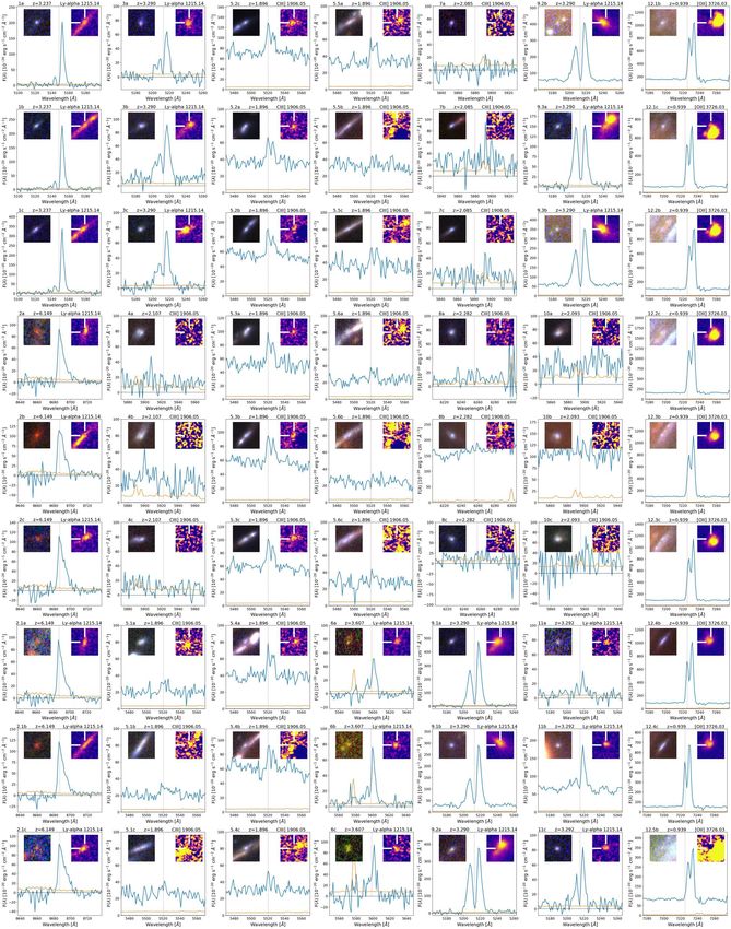
A&A proofs: manuscript no. 39466corr

1. Introduction                                                            zini 2017), thus suggesting that a significant fraction of the star
                                                                           formation of the Universe in the first Gyrs took place in these
The key capabilities of extremely large telescopes (ELTs) for the          systems. Therefore, if reionization was mainly driven by star for-
exploration of the distant Universe will provide unprecedented             mation – which is mostly confined to bound star clusters – then
access to faint luminosities (thanks to a large collecting area) and       it is plausible that young star clusters played an essential role in
angular resolution down to ∼ 10 milliarcsec (mas) thanks to the            this process (e.g., Ricotti 2002; Boylan-Kolchin 2018; Bik et al.
technology of adaptive optics (AO). In the near future, the im-            2018; Vanzella et al. 2020a; Herenz et al. 2017a).
minent launch of the James Webb Space Telescope (JWST) will                     For the reasons described above, a census of gravitationally-
open up a new wavelength domain redward of the K−band that                 bound young star clusters at high redshift would represent a big
is crucial for capturing rest-frame optical lines well within the          step forward in this investigation. Observationally, such a census
reionization epoch. These future facilities will allow us to rou-          requires improvements in angular resolution and depth in the rest
tinely analyze the internal structures of high-redshift galaxies at        frame UV with HST. Observations in the rest frame optical and
unprecedented small spatial scales. With a typical point spread            longer wavelengths (JWST and ALMA) will then be necessary
function (PSF) of ∼ 10 mas (milli-arcsecond) and a pixel scale             to understand their physical properties in detail.
of 4 mas per pixel, the high-redshift galaxies that remain unre-
                                                                                Even though angular resolution of 10-20 mas in the rest
solved today will finally be dissected into resolution elements of
                                                                           frame UV is currently not attainable overall, significant progress
80 (60) parsec at a redshift of 3 (6), eventually providing con-
                                                                           has been made in terms of depth with the VLT, which is per-
straints down to spatial scales of ∼ 20 (30) pc per pixel (e.g.,
                                                                           forming very deep spectroscopy of the faintest sources in what
E-ELT/MAORY-MICADO). In this regard, star-forming com-
                                                                           is currently the deepest field obtained with Hubble (the Hubble
plexes (< 200 pc size) at high redshift and high mass star clus-
                                                                           Ultra Deep Field, HUDF, Beckwith et al. 2006; Illingworth et al.
ters (e.g., < 30 pc radius) will be accessed and compared to local
                                                                           2013; Koekemoer et al. 2013). The initial results from an ex-
similar star-forming regions, allowing for detailed studies of (1)
                                                                           tended integration time (> 30 hours), obtained with the VLT
star-formation modes (e.g., location and spectral signatures of
                                                                           multi-unit spectroscopic explorer (MUSE, Bacon et al. 2012)
massive stars); (2) the presence of high-ionization lines and the
                                                                           in the HUDF, have been presented in a series of recent works
related ionization photon production efficiency (e.g., Bouwens
                                                                           (e.g., Bacon et al. 2017; Inami et al. 2017; Maseda et al. 2018,
et al. 2016; Amorín et al. 2017; Senchyna et al. 2017; Cheval-
                                                                           2020; Wisotzki et al. 2018; Kusakabe et al. 2020; Feltre et al.
lard et al. 2018; Senchyna et al. 2019; Lam et al. 2019; Senchyna
                                                                           2020)2 , confirming redshifts for galaxies as faint as magnitude-
et al. 2020b); and (3) interactions with the surrounding medium
                                                                           30 (Brinchmann et al. 2017), including a set of “HST-dark”
(feedback), including the capacity to modulate the opacity of the
                                                                           MUSE sources with detected emission lines (typically Lyα) with
interstellar medium to ionizing radiation up to circumgalactic
                                                                           no detection of HST counterparts (Inami et al. 2017; Mary et al.
scales (which is key for the escape of ionizing photons, e.g.,
                                                                           2020). The VLT/MUSE coverage has revolutionized the study
Erb 2015; Grazian et al. 2017; Vanzella et al. 2020a; He et al.
                                                                           of the high-redshift Universe at z < 6.65 in the post-reionization
2020). These are all key ingredients in the pursuit of answers to
                                                                           epoch (Bacon 2020).
two of the most pressing questions in current observational cos-
mology: i) what sources reionized the Universe (e.g., Robertson                 A complementary approach is the use of gravitational lens-
et al. 2015; Giallongo et al. 2015; Meyer et al. 2020; Eide et al.         ing magnification (µ) (e.g., Bradley et al. 2014; Atek et al. 2014,
2020; Dayal et al. 2020); ii) how globular clusters formed (Ren-           2015, 2018; Treu et al. 2015; Karman et al. 2015, 2017; Caminha
zini et al. 2015; Renzini 2017; Pfeffer et al. 2018, 2019; Calura          et al. 2019; Erb et al. 2019; Richard et al. 2014) provided by clus-
et al. 2019; Bastian & Lardo 2018); iii) and how these two ques-           ters of galaxies, which makes background sources brighter and
tions might be related to each other (e.g., Ricotti 2002; Schaerer         larger on the sky, thus allowing for a much higher effective res-
& Charbonnel 2011; Katz & Ricotti 2013; Boylan-Kolchin 2018;               olution than in blank fields with the same observational setup.
Ma et al. 2020; He et al. 2020).                                           For example, the combination of (1) MUSE integral field spec-
                                                                           troscopy; (2) lensed fields; and (3) deep multi-frequency HST
    Indeed, it has been established in the local Universe that
                                                                           imaging (such as the Hubble Frontier Fields, HFF hereafter, Lotz
the fraction of forming stars located in gravitationally bound
                                                                           et al. 2017; Koekemoer et al. 2014) has led to the confirmation
star clusters (also known as cluster formation efficiency, Γ1 ),
                                                                           of an unprecedented number of multiple images per field up to a
increases as the star-formation rate surface density increases
                                                                           redshift of z ' 6.7 (Caminha et al. 2017; Lagattuta et al. 2019).
(Adamo et al. 2017, 2020a,b); this, in turn, relates to the increas-
                                                                           These identifications are crucial for constructing high-precision
ing gas pressure in high gas surface density conditions (Krui-
                                                                           lens models. Such observations have given us a first glimpse of
jssen 2012; Li et al. 2018). It has also been proposed that Γ
                                                                           what will be accessible with ELTs or extreme AO facilities such
positively correlates with redshift, such that, on average, high-
                                                                           as VLT/MAVIS3 in blank fields.
density conditions and merger rate in the high redshift Universe
would favor Γ > 30 − 40%, whereas it is of a few percent at low                 The sub-kpc spatial resolution provided by lensing magnifi-
redshift (z < 2) (e.g., Pfeffer et al. 2018). Similar arguments,           cation revealed spatial variations of, for instance, Lyα emission
based on the present-day volume density of globular clusters               along the arcs (e.g., Claeyssens et al. 2019), and, in combina-
projected back in time, suggest that at z & 5, about half of the           tion with HST deep imaging, it allowed the detection of faint
stellar mass of the Universe was located in star clusters (Ren-            lensed sources (e.g., Mahler et al. 2018). As an interesting ex-
                                                                           ample, some star-forming complexes, discovered in the HFFs,
  ?                                                                        have characteristic sizes smaller than 100 pc along with other
     E-mail: eros.vanzella@inaf.it
 ??
     Based on observations collected at the European Southern Observa-     physical parameters that make them good candidates for glob-
 tory for Astronomical research in the Southern Hemisphere under ESO       ular cluster precursors (Vanzella et al. 2016, 2017b,c). In fact,
 programmes ID 0100.A-0763(A) (PI E. Vanzella), 094.A-0115B (PI J.
                                                                            2
 Richard), 094.A-0525(A) (PI F.E. Bauer).                                     The      complete     list  is    available     here:    http://muse-
???
     Hubble Fellow                                                         vlt.eu/science/publications/
  1
    Γ is defined as the cluster formation rate (CFR) divided by the star    3
                                                                              http://mavis-ao.org/mavis/ and https://arxiv.org/abs/2009.09242 for
 formation rate (SFR) of the hosting galaxy (Bastian 2008).                the Phase A Science Cases.

Article number, page 2 of 43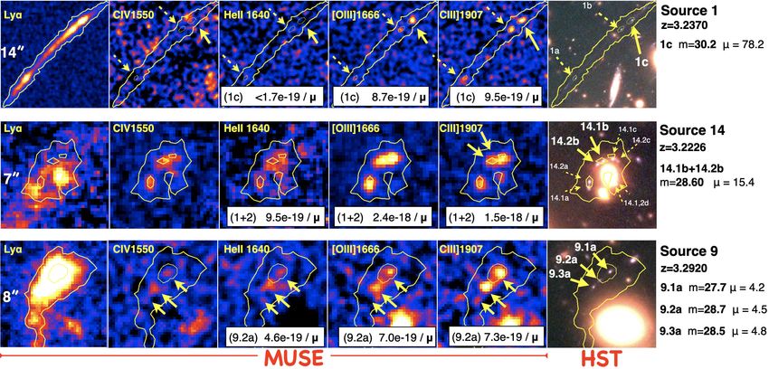
E. Vanzella et al.: Star-forming complexes at cosmological distance

along the maximum tangential stretch provided by strong lens-          lensing (where µ is the magnification factor). With the addition
ing, the effective resolution of HST reaches a few tens of pc,         of publicly available data in the south-west region of the same
while the boosted signal-to-noise ratio (S/N) enables a morpho-        galaxy cluster (with 11-hour integration; see Sect. 2.3), the num-
logical analysis that would be impossible in blank fields. One         ber of confirmed multiple images increases to the unprecedented
such a case is the compact object behind MACS J0416, identified        number of 182 in the redshift range of 0.9 < z < 6.2. A new
as a young massive star cluster with an intrinsic (i.e., delensed)     lens model based on this set of images is presented in an ac-
magnitude of 31.3 and effective radius smaller than 13 pc, which       companying paper by Bergamini et al. (2020). Soon after this
is hosted in a dwarf galaxy at z = 6.149 (Vanzella et al. 2019;        paper appeared on astro-ph, Richard et al. (2020) submitted a pa-
Calura et al. 2020). Similarly, high-redshift star-forming clumps      per presenting an atlas of MUSE observations of 12 clusters and
(< 200 pc size) have been identified in various lensed fields,         corresponding lens models. This study included the new MUSE
suggesting that a hierarchically structured star-formation topol-      deep observations of MACS J0416 presented here.
ogy emerges whenever the angular resolution increases (see also,           The present work is structured as follows: Section 2 presents
Livermore et al. 2015; Kawamata et al. 2015; Rigby et al. 2017;        the MUSE observations and data reduction. Section 3 presents
Johnson et al. 2017; Dessauges-Zavadsky et al. 2017; Cava et al.       the full set of multiple images. Section 4.1 focuses on the sam-
2018; Zick et al. 2020). In a recent spectacular case, a highly        ple of star forming clumps identified among the multiple images,
magnified, finely structured giant arc has been identified as the      and Section 4.2 details the spectral stacking and the most rele-
first example of a young (3 Myr old) massive star cluster at           vant high-ionization lines. Individual sources are presented in
z = 2.37, directly detected in the Lyman continuum (λ < 912 Å)         Section 5, highlighting two examples of extremely small objects
and contributing to the ionization of the IGM (Vanzella et al.         as potential gravitationally bound star clusters. We assume a flat
2020a; Rivera-Thorsen et al. 2019; Chisholm et al. 2019).              cosmology with Ω M = 0.3, ΩΛ = 0.7 and H0 = 70 km s−1 Mpc−1 .
     There are two key aspects in the study of the distant Universe
in lensed fields driven by MUSE integral field spectroscopy: (1)
the 10 × 10 field of view integral field unit (IFU) provides spec-     2. The MUSE Deep Lensed Field: Observations and
troscopic redshifts without any target pre-selection, significantly       data reduction
enlarging the discovery space (the identification of globular clus-
                                                                       Deep MUSE (Bacon et al. 2012) observations were allocated in
ter precursors and extremely faint sources with intrinsic magni-
                                                                       period 100 (Prog.ID 0100.A-0763(A) − PI E. Vanzella) on a sin-
tude > 31 are two examples among a number of others); and (2)
                                                                       gle pointing covering the north-east (NE) lensed region of the
dozens of multiple images can be easily identified by the IFU in a
                                                                       HFF galaxy cluster MACS J0416 (Figure 1). Out of a total of
single observation, even when distorted or extended. This yields
                                                                       19 observing blocks (OBs) that were scheduled (22.1h, includ-
a vast gain in efficiency compared to traditional target-oriented
                                                                       ing overhead), 16 have been successfully acquired with quality
“multi-slit spectroscopy,” at least when a large field of view is
                                                                       A or B (84%).4 Table 2 lists the log of the observations that
not required and when the density of targets is high.
                                                                       were executed in the period between November 2017 till Au-
     The dramatic increase in spectroscopically confirmed multi-       gust 2019. 14 OBs out of 16 have been acquired with the as-
ple images is key for producing robust magnification maps with         sistance of Ground Layer Adaptive Optics (GLAO) provided by
lens models, with a much improved understanding of the system-         the GALACSI module. Each exposure was offset by fractions
atic uncertainties affecting magnification values and their gradi-     of arcseconds and rotated by 90 degrees to improve sky sub-
ents across the image (e.g., Grillo et al. 2015, 2016; Meneghetti      traction. The image quality was very good, spanning the range
et al. 2017; Caminha et al. 2017; Atek et al. 2018; Treu et al.        between 000. 4 − 000. 8, with a median PSF full width at half maxi-
2016). This remains a critical step for inferring intrinsic physi-     mum (FWHM) of 000. 6. The same NE field of the galaxy cluster
cal properties or the geometry of highly magnified galaxies.           was observed within a GTO program (Prog.ID 094.A-0115B, PI:
     The confirmation of lensed sources with intrinsic magnitudes      J.Richard) in November 2014, for a total of two hours split into
in the range of 30−33 via Lyα emission shows that sources with-        four exposures (Caminha et al. 2017). We added the 2014 dataset
out HST imaging counterparts are common in lensed fields and           to our MUSE data, eventually producing a total integration time
at fluxes fainter than those of similar HST−dark MUSE sources          of 17.1h on-sky with a final optimal image quality of 000. 6. In
found in the HUDF. An example is the high equivalent width             the following, we refer to this deep pointing as the MUSE Deep
(> 1000 Å rest-frame) Lyα arclet at z = 6.629, straddling a caus-      Lensed Field (MDLF).
tic, which is confirmed in the MDLF. The HST counterpart is
barely detected in HST imaging (with an observed magnitude of
                                                                       2.1. Data reduction
& 31 at 2σ level), which corresponds to an intrinsic magnitude
fainter than 35. This suggests that such star-forming complex          We used the MUSE data reduction pipeline version 2.8.1 (Weil-
possibly hosts extremely metal-poor (or Pop III) stellar popula-       bacher et al. 2014) to process the raw data and create the final
tions (see Vanzella et al. 2020b, for details). This is perhaps the    stacked data-cube. All standard calibration procedures were ap-
most compelling example of a blind spectroscopic detection, as         plied to the science exposures (i.e., bias and flat field corrections,
it would be impossible to place a slit over such an object based       wavelength and flux calibration, etc.). In order to reduce the re-
on deep imaging alone.
                                                                       4
     To push the frontier of integral field spectroscopy of the           The quality control of OBs executed in service mode is based on the
high redshift Universe, we present in this work the MUSE               specified constraints in the OB for airmass, atmospheric transparency,
                                                                       image quality and seeing, Moon constraints, twilight constraint, as well
Deep Lensed Field over the North-East part of the Hubble
                                                                       as Strehl ratio for Adaptive Optics mode observations (as requested).
Frontier Field galaxy cluster MACS J0416.1−2403 (hereafter             If all constraints are fulfilled, the OB is marked with the grade "A",
MACS J0416). We show that a total integration of 17.1 hours in         while the "B" quality control is assigned if some constraint is up to 10%
a single MUSE pointing on the magnified region of the cluster          violated. The observations with quality control grades A or B are com-
produces point-like source detection that would require > 100          pleted, while those with quality control grade "C" (out of constraints)
(µ > 2.5) to > 1000 (µ > 7.5) hours of integration without             are re-scheduled and may be repeated (www.eso.org).

                                                                                                                  Article number, page 3 of 43
A&A proofs: manuscript no. 39466corr

Fig. 1. Color image of the HFF galaxy cluster MACS J0416 shown in the main panel (red, green, and blue as F105W, F814W, and F606W,
respectively). The MDLF centered in the north-east part of the cluster is outlined by the yellow contour (17.1h integration time), while the blue
contour shows the observation in the south-west (11-hour integration, PI Bauer, 094.A-0525(A)). The red circles mark the positions of the 182
multiple images used to constrain the lens model (Bergamini et al. 2020). The insets show zoomed examples of strongly lensed objects with
detected clumps in the redshift range of 1.5 < z < 6.5 (discussed in detail in Sect 4). In each inset, the catalog ID (red number) and redshift
are indicated, while the segment marks the 000. 3 scale. Yellow circles mark two images not covered by MUSE, which are however included in the
multiple images sample due to their mirroring lensing properties.

maining instrumental signatures due to slice-to-slice flux varia-         1.25 Å/pixel and a fairly constant spectral resolution of 2.6 Å
tions of the instrument, we used the self-calibration method. This        over the entire spectral range. The total integration time is 17.1h,
method is based on the MUSE Python Data Analysis Framework                with an image quality of 000. 6, as measured on two stars available
(Bacon et al. 2016) and implemented in the last versions of the           in the field.
standard reduction pipeline provided by ESO. The final astrome-
try was performed matching sources detected with SExtractor
(Bertin & Arnouts 1996) in the white image of the final data-             2.2. Depth of the MDLF
cube and detections in the HFF filter F606W image. Finally, we
applied the Zurich Atmosphere Purge (Soto et al. 2016) on the
data-cube in order to remove the still remaining sky residuals.           The performances and the depth achievable with the VLT/MUSE
                                                                          instrument have been well monitored in the past few years from
      Four OBs, indicated as “NOAO” in Table 2, have been ob-
                                                                          extensive observations, from a few to dozens of hours of in-
served with an average natural seeing (i.e., without GLAO) of
                                                                          tegration time (e.g., Inami et al. 2017). In particular, the very
000. 6, and simply included in the co-addition of all OBs following
                                                                          deep campaign performed in the Hubble Ultra Deep field, HUDF
the procedure described above. For these datacubes no Raman
                                                                          (e.g., Bacon et al. 2017; Maseda et al. 2018, and references
lines due to the laser are present, especially in the wavelength
                                                                          therein), suggest a growing S/N that is fully in line with the ex-
range of 5800 − 6000 Å. However, the final co-added cube is               pected integration time (see also, Bacon et al. 2015). Under the
dominated by OBs obtained with GLAO (14 out of 18).                       assumption of similar observing conditions and data reduction
      The final data-cube has a spatial pixel scale of 000. 2, a spec-    technique, a proper rescaling of the depth reported from deep
tral coverage from 4700 Å to 9350 Å, with a dispersion of                 GTO program (e.g., Inami et al. 2017) would suggest a line flux
Article number, page 4 of 43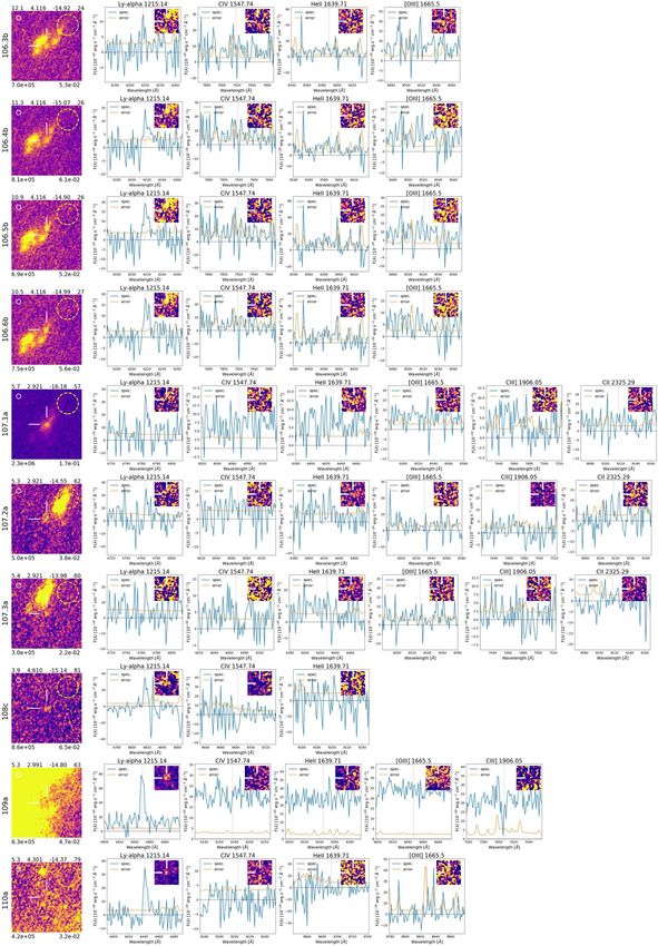
E. Vanzella et al.: Star-forming complexes at cosmological distance

Table 1. Summary of the MDLF observations

   Date                     Quality    OB Name
                            MDLF
   22/23-Nov-2017             A        WFM_J0416_NOAO_1
   10/11-Jan-2018             A        WFM_J0416_NOAO_2
   21/22-Feb-2018             C        WFM_J0416_NOAO_3
   12/13-Mar-2018             X        WFM_J0416_AO_1
   4/5-Nov-2018               A        WFM_J0416_AO_10
   5/6-Nov-2018               B        WFM_J0416_AO_1
   5/6-Nov-2018               A        WFM_J0416_AO_2
   6/7-Nov-2018               A        WFM_J0416_AO_4
   2/3-Dec-2018               A        WFM_J0416_AO_11
   4/5-Dec-2018               A        WFM_J0416_AO_13
   12/13-Dec-2018             A        WFM_J0416_AO_14
   11/12-Jan-2019             B        WFM_J0416_AO_5
   16/17-Jan-2019             C        WFM_J0416_AO_6
   25/26-Jan-2019             A        WFM_J0416_AO_6
   27/28-Feb-2019             A        WFM_J0416_AO_17
   28-Feb/1-Mar-2019          A        WFM_J0416_AO_7
   3/4-Mar-2019               A        WFM_J0416_AO_8
   2/3-Aug-2019               A        WFM_J0416_AO_9
   30/31-Aug-2019             A        WFM_J0416_AO_18
                             GTO
   17-Dec-2014                A        WFM_J0416_NOAO
   17-Dec-2014                A        WFM_J0416_NOAO

Notes. Log of the observed OBs. The typical exposure time (on sky) of
each OB is 3340s. The bottom two rows refer to the previous two hours    Fig. 2. Top panel: White-light image of the MDLF is shown together
of observation from the GTO. The column “OB Name” indicates the          with the 600 non-overlapping apertures placed in empty zones not in-
observing mode ("WFM" = wide field mode) and the use (or not) of the     tercepting visible objects in the image. The corresponding median value
adaptive optics "AO/NOAO", meaning "on/off".                             calculated at each wavelength and consistent with the zero level (black
                                                                         line), 16th−84th percentiles (red and blue lines), and the rms (green
                                                                         line) are reported below the white image. Apertures have a diameter of
limit for our 17.1h MDLF of ' 2 × 10⁻¹⁹ erg s−1 cm−2 at 3σ,              000. 8 and the statistics is computed on each aperture by collapsing slices
λ = 7000 Å and within an aperture of 000. 8 diameter.                    within dv=300 km s−1 . The pattern of the sky emission lines is evident.
    Similarly to what described by Herenz et al. (2017b), we then        The increased noise in the range of 5800 < λ < 6000 Å is due to the
carried out a posteriori checks of the noise fluctuation of the re-      emission of the laser used for ground layer AO.
duced data cube (i.e., after the full data reduction) by placing 600
non-overlapping apertures (of 000. 8 diameter) on positions visu-
ally extracted from the white image (obtained by collapsing the          quired to obtain the same S/N achievable in lensed fields is ob-
full wavelength range) and not intercepting evident sources. The         tained by rescaling the MDLF integration to µ2 . T(MDLF) × µ2 ,
location of the apertures is plotted over the white image in Fig-        where T(MDLF)=17.1h. Figure 3 shows the texp map needed
ure 2. We then calculated the flux within each aperture by inte-         to obtain the same depth of MDLF without lensing. It is widely
grating it over a velocity width of dv=300 km s−1 (kept constant         known that strong lensing boosts the detection of faint sources
across the full wavelength range), typical of Lyα emission in            and represents a complementary approach to observations in
high redshift galaxies. The mean and rms, as well as the median          blank fields, however, deep observations like the MDLF allow us
and the 68% central interval within the 16th and 84th percentiles        to reach equivalent texp ' 100 h even in regions where magnifi-
within the 600 apertures, were extracted at each wavelength with         cation is modest, µ ∼ 2 − 3. The 90% of the MDLF field of view
an incremental step of 1.5 Å. Figure 2 shows the median and              is equivalent, in terms of depth, to > 100 h of integration in non-
percentiles as a function of wavelength. The pattern of the sky          lensed fields (with the most magnified regions pushing texp up
spectrum clearly emerges, as well as the increased noise in the          to 1000 h where µ > 7.7). The same figure also shows the equiv-
wavelength range of 5800 Å−6000 Å due to the GLAO sodium-                alent 3-sigma line flux limit after rescaling to texp. Line fluxes
based laser. We derive a 3σ limit of 1.5 × 10⁻¹⁹ erg s−1 cm−2            down to a few 10−20 erg s−1 cm−2 can be probed in regions with
at 7000 Å (where no OH sky lines are present) within an aper-            large magnification (texp > 200 hours). Such a depth allows us
ture of 000. 8 diameter and collapsed over 300 km s−1 along the          to detect high-ionization lines on individual objects with intrinsic
wavelength direction.                                                    magnitudes 27 − 30 (see Sect. 5). The outer regions of the galaxy
    The magnification across the field provided by the gravita-          cluster at relatively low-µ have the advantage to be relatively
tional lensing effect further decreases the detectable line flux         free from contamination by galaxy cluster members and are less
limit in the MDLF when compared to the Hubble Ultra Deep                 affected by large uncertainties on the magnification, being far
Field (Bacon et al. 2017). Assuming a point-like emitting source         from the critical lines. The major drawback of strongly lensed
and that, at first order, the magnification is the ratio between the     fields is the smaller intrinsic area probed behind the lens when
observed flux and the de-lensed(intrinsic) one, µ = Fobs /Fintr ,        compared to the non-lensed fields. An illustration of this effect
the equivalent integration time (texp) in absence of lensing re-         is shown in Figure 4, which shows the cumulative surface area
                                                                                                                     Article number, page 5 of 43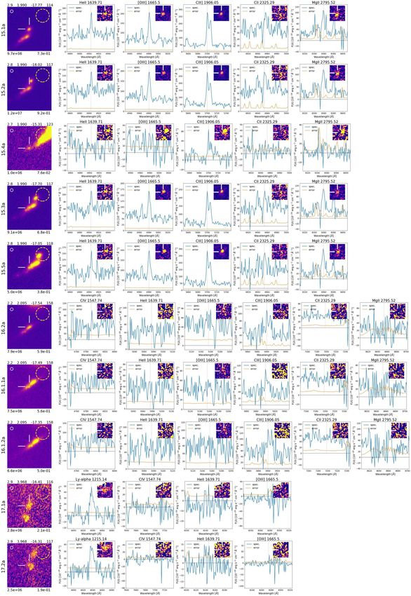
A&A proofs: manuscript no. 39466corr

on the lens plane probed by the MDLF as a function of magni-
fication (in magnitude units). The surface area decreases rapidly
with µ reaching half of its original coverage when µ ∼ 6.3.

2.3. The MUSE pointing in the South-West: MUSE-SW
Relatively deep observations in the SW region of the same
galaxy cluster (J0416) were carried out under the ID 094.A-
0525(A) program (PI: F.E. Bauer). This includes 58 exposures
of approximately 11 minutes each, executed over the period Oc-
tober 2014 − February 2015. We use the same reduced data-cube
described in Caminha et al. (2017). Despite a relatively long ex-
posure in the SW pointing (formally 11h integration), the S/N of
the spectra does not scale according to expectations, resulting to
an equivalent integration of ∼ 4 hr only. Caminha et al. (2017)
attribute this inconsistent depth to the significantly worse seeing
of the SW pointing (100 vs. typically 000. 6) and the large number
of short exposures used which, due to residual systematics in
the background subtraction, did not yield the expected depth in
the coadded data-cube. As discussed in Bergamini et al. (2020),
the depth provided by the MDLF produces a major gain in the
number of bona fide multiple images, as discussed in the next
section.                                                                     Fig. 4. Cumulative surface area of the MDLF in the image plane as a
                                                                             function of magnification in magnitude units (µ[mag] = 2.5 log10 (µ))
                                                                             for redshift 6 (orange line) and 3 (blue line). Arrows mark the magni-
                                                                             fications corresponding to the exposure time (=100, 200, 1000, 10000
                                                                             hours) as shown in Figure 3, necessary for obtaining the same depth of
                                                                             the MDLF without lensing.

                                                                             imaged objects. This process was based on (a) visual inspec-
                                                                             tion of color images, (b) the assistance by the lens model which
                                                                             was progressively refined (Bergamini et al. 2020), (c) the AS-
                                                                             TRODEEP photometric redshift catalog (Castellano et al. 2016;
                                                                             Merlin et al. 2016). Different versions of continuum-subtracted
                                                                             cubes were generated varying the width of the central window
Fig. 3. Left: Equivalent exposure time needed to reach the same S/N          within which slices are collapsed (with typical dv=300-500 km
probed with the MDLF without lensing, assuming point-like sources            s−1 ) and the redward and blueward regions used to estimate the
at z = 6. Contours of iso-exposure are shown (100, 200, 1000 hours
equivalent integration). We note that the MDLF is equivalent to 100 h        continuum level, typically with widths of 20 − 30 Å.
integration in blank fields already with modest magnification, µ ∼ 2.5.           The MDLF observations allowed us to increase significantly
Right: Map of the 3-sigma line flux limit adopting a velocity width of       the number of multiple images in the NE region of the cluster
300 km s−1 and a circular aperture of 000. 6 diameter, based on the same     and triple the S/N of the previous 2h exposure data-cube from
assumptions as in the left panel. The color-bar indicates the log of flux    GTO. Individual sources contain in some cases multiply imaged
values in erg s−1 cm−2 , whereas the three contours correspond to the flux   clumps (see, e.g., Figure 5 and Sect. 4), in which more than one
(flx) of 10−19 , 5 × 10⁻²⁰ , and 10−20 erg s−1 cm−2 .                        family can be part of the same high-z galaxy.5 In particular, the
                                                                             total number of families increases to 66, with the new ones cov-
                                                                             ering the redshift range of 0.9 < z < 6.2. As a result, the number
                                                                             of individual high redshift galaxies generating the set of multiple
3. Catalog of multiple images                                                images is lower than 66, amounting to 48 independent sources.
                                                                             The arclet at z = 6.629 has not been included among the con-
In combining MUSE-SW and the initial two hours of integration                straints of the model because no clear HST counterparts have
in the north-east from GTO observations, Caminha et al. (2017)               been currently identified (see Vanzella et al. 2020b).
identified 37 galaxies producing 102 multiple images in the red-
shift range of 1 < z < 6.2. The MDLF and a careful identification
                                                                             5
of confirmed additional lensed families led to an unprecedented                 A family is defined as a set of multiple images of the same back-
set of 182 multiple images, spanning the same redshift range                 ground object. An object can be either a single galaxy or a single sub-
of 0.9 < z < 6.2. To search for new sources, we followed the                 component of the same galaxy (e.g., a clump). For example, source
procedure described in Caminha et al. (2017). Firstly, using our             5 has 6 families with three multiple images each (a,b,c): 5.1(abc),
                                                                             5.2(abc), 5.3(abc), 5.4(abc), 5.5(abc), and 5.6(abc), which have been
lens model we looked in the vicinity of the predicted positions of
                                                                             used to constrain the lens model. In some cases, HST single-band imag-
multiple images of families partially lacking spectroscopic infor-           ing reveals that individual families are further split into two knots,
mation. This led us to complete the spectroscopic information of             which are labeled with an extra digit, e.g., 5.1.1 and 5.1.2 or 5.6.1 and
several lensed systems. Secondly, new sources have been identi-              5.6.2. These extra knots are not used as constraints in the lens model.
fied by exploring narrow-band continuum subtracted cubes and                 Source 1, made of multiple images 1a, 1b, and 1c corresponds to only
analyzing spectra extracted at the position of candidate multiply            one family.

Article number, page 6 of 43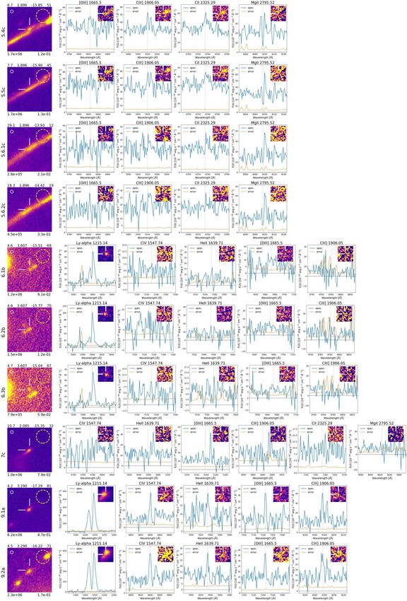
E. Vanzella et al.: Star-forming complexes at cosmological distance
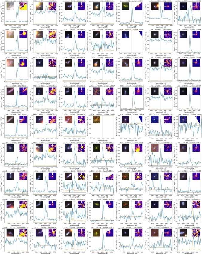
Fig. 5. Eight clumps identified for source 5 are marked with IDs 5.1.2,
Fig. 6. Examples of the most prominent multiply imaged Lyα emitting
5.1.1, 5.2, 5.3, 5.4, 5.5, 5.6.2, 5.6.1 and indicated on both sides of the
regions spatially resolved in the MDLF. Multiple images are indicated
critical line (red dashed line), labeled as group C (5c) and B (5b). The
as A, B and C (connected with dotted lines) with color-coded contours
top-left inset shows on the same scale the least magnified image 5a, in
at the 2σ level calculated on the continuum-subtracted narrow-band
which all the corresponding clumps can be recognized. The bottom-
MUSE images, centered on Lyα emission. In the case of source 14,
right insets show the continuum-subtracted narrow-band images ex-
the Civ λ1548 emission is shown instead of Lyα (being deficient in Lyα
tracted from MUSE around the wavelength of the most prominent high
emission (see also Figure C.1 and discussion in Vanzella et al. 2017c).
ionization emission lines.
For more details about sources 103 and 106, see Figure 7.
As discussed in Sect. 4, a close inspection of the confirmed
multiple images in deep HST data reveals a significant fraction (e.g., relative intensities of the blue and red peaks) will be pre-
of multiply imaged clumps emerging from each high-z galaxy. sented in a future work. An example showing the most promi-
Those that are firmly identified are included as constraints in the nent cases in the MDLF is reported in Figure 6, where multiple
lens model. The number of clumps typically increases where images of Lyα nebulae at z = 3 − 6 extend along the tangen-
magnification increases, eventually making them individually tial direction and possibly include even fainter clustered sources
recognizable (enhanced spatial scale) and detectable (enhanced (currently not detected on HST images, e.g., Mas-Ribas & Dijk-
S/N). The inclusion of multiple clumps is particularly useful for stra 2016) contributing to the Lyα emission. One of them, source
better constraining the position of critical lines and the high mag- 9, shows a spatially-varying multi-peak Lyα emission and neb-
nification values in these regions. Such examples are families 5 ular high-ionization lines emerging from three well-recognized
at z = 1.8961 (see Figure 5) and source 12 at z = 0.9390, in knots (this system was already presented in Vanzella et al. 2017a
which the large magnification close to the critical lines is bet- using much shallower MUSE observations).
ter sampled by a high spatial density of local constraints corre- The depth of the MDLF also allows us to confirm sources
sponding to star-forming clumps (see Bergamini et al. 2020 for without Lyα emission, down to magnitude ' 26. One exam-
more details). ple is source 106b at z = 4.116 (see Figure 7), for which the
At the end of this process, the spectroscopic confirmation continuum-break is clearly detected, its redshift is measured by
of new high-z galaxies and the addition of individual clumps cross-correlating the spectrum with high-z templates6 , and found
increase the total number of multiple images used for the lens consistent with the spatially offset Lyα nebula. Interestingly, the
model to 182 (66 families), spanning the redshift range of 0.9 < spectroscopic redshift is also in very good agreement with the
z < 6.2. Bergamini et al. (2020) present the details of the lens photometric redshift derived from ASTRODEEP, z phot = 4.20
model, which is currently the one exploiting the largest number (Castellano et al. 2016). As discussed in the Sect. 4, source 106b
of spectroscopically confirmed constraints for any galaxy clus- is also a good example of how a galaxy can be resolved into sev-
ter. It includes 80 additional multiple images compared to the eral sub-components by strong lensing (at least six star-forming
previous model and 213 confirmed galaxy cluster members (20 regions of ∼ 100 − 200 parsec size).
more than in the previous model), by reproducing the positions
of all 182 multiple images with an rms accuracy of only 000. 40. In 3.1. The full MUSE spectroscopic catalog
Appendix A, we present the details of all multiple images, show-
ing, for each of them, the HST cutouts and MUSE narrow band In addition to the set of multiple images specifically used by
continuum-subtracted imaging at the wavelength position of the Bergamini et al. (2020) to constrain the lens model, we also re-
most relevant emission lines. leased a version of the MUSE spectroscopic catalog that includes
The Lyα emission is often spatially resolved and extends be- all the sources we identified in the MUSE datacubes. By com-
yond the HST counterpart down to the very faint fluxes permitted
by lensing magnification. A dedicated analysis of the spatially 6
Redshifts have been measured using the Eazy package within the
extended Lyα emission and intrinsic spatially-varying profiles Pandora environment (Garilli et al. 2010).
Article number, page 7 of 43
A&A proofs: manuscript no. 39466corr

Fig. 7. Lyα nebulae (red contours at 2-σ level) including images 106(a,b) and 103(a,b), belonging to the same physical structure at z=4.116, are
shown in the main panel (HST ACS/F814W band). In the top-right inset, the lensed galaxy 106b broken in six clumps is shown; the smaller ones
(2 − 6) have intrinsic UV magnitude ' 30.5 − 31 (corresponding to MUV ' −15) and intrinsic sizes of the order of (or smaller than) 100 pc along
the tangential stretch, as indicated by the ruler. The bottom inset shows two one-dimensional spectra extracted from the MDLF. One is on galaxy
106b (within a circular aperture of 1.200 diameter, see magenta circle). We note the ultraviolet continuum of 106b with F814W = 26.01 ± 0.03 is
well-detected (magenta line) above the zero level (black dashed line), and its continuum-break confirmed at z=4.116. The top spectrum is extracted
from a nearby region showing Lyα emission without HST counterpart (green circle with 1.200 diameter, labeled as #1), vertically shifted at position
10 for illustrative purposes. The error spectrum is shown in blue at the bottom to highlight the location of the sky emission lines. The shaded band
marks the wavelength region affected by the GLAO sodium-based laser.

bining the MDLF and MUSE-SW pointing, this catalog contains                the brightest clump of a complex system at z = 2.810 showing
424 individual objects, spanning the redshift interval up to z=6.7,        various knots. Its observed magnitude of 24.16 (25.7 intrinsic)
thus extending the sample of 182 multiple images (48 objects).             makes it relatively bright, however, the increased S/N provided
Faint sources with observed magnitude down to m1500 > 28 have              by the MDLF reveals multiple spectral features (if compared to
been confirmed, corresponding to intrinsic m1500 > 29 − 30 in              the initial four-hour integration), such as the broad Heiiλ1640
the case of µ ' 3 − 6. The typical error at this magnification             and Civ P-Cygni profile, both indicating the presence of strong
regime is less than 20%, implying that the error on the intrinsic          stellar winds arising from massive O and WR stars, with a possi-
magnitude is mainly dominated by the photometric uncertainty               bly further signature of P-Cygni of Nvλ1240 indicative of ages
(for the given cosmology).                                                 younger than 5 Myr (e.g., Senchyna et al. 2020a; Vanzella et al.
    Figure 8 shows three examples of the aforementioned cases.             2020a; Chisholm et al. 2019). Appendix A presents the spectro-
In particular, the spectra of two of these confirmed very faint            scopic catalog of all high-z objects, including some that are not
sources at z = 3.613 (ID = -99) and z = 2.927 (ID = 2046)                  multiple images.
(in magenta and red colors respectively) have intrinsic magni-
tudes m1500 = 31.1 and 29.6, with an error of 0.3 mag (includ-
ing the magnification uncertainty). ID=2046 also shows an ex-              4. Clumpy high-z galaxies
tremely blue ultraviolet slope with a relatively small error, as           A common morphological property of high redshift star-forming
estimated from the HST F606W, F814W and F105W photomet-                    galaxies is the presence of clumps (Zanella et al. 2015, 2019),
ric bands, β = −2.9 ± 0.2 (Fλ ' λ−β , Castellano et al. 2012).             that seem to emerge whenever the angular resolution increases.
Interestingly, the same object also shows a very large equiva-             Strong gravitational lensing reveals such clumps down to a ∼
lent width of the Lyα (220 ± 25 Å) and the presence of faint               100 pc scale (Livermore et al. 2015; Rigby et al. 2017; Cava et al.
nebular Civλ1548, 1550 doublet, associated to an object with an            2018) that further continue fragmenting down, approaching the
estimated stellar mass of a few million solar masses (106.8 M ).           sizes of massive stellar clusters (. 30 pc) in high magnification
    Another example in Figure 8 shows that deep MUSE obser-                regimes, µ > 10 (Vanzella et al. 2019, 2020a; Johnson et al.
vations of (intrinsically) relatively bright, moderately magnified         2017).
galaxies (µ ' 3−6) reveal or consolidate spectral features clearly             The identification of star-forming clumps in the secure mul-
associated with the presence of massive stars. Source 2357 is              tiple images discussed here has been visually performed by look-
Article number, page 8 of 43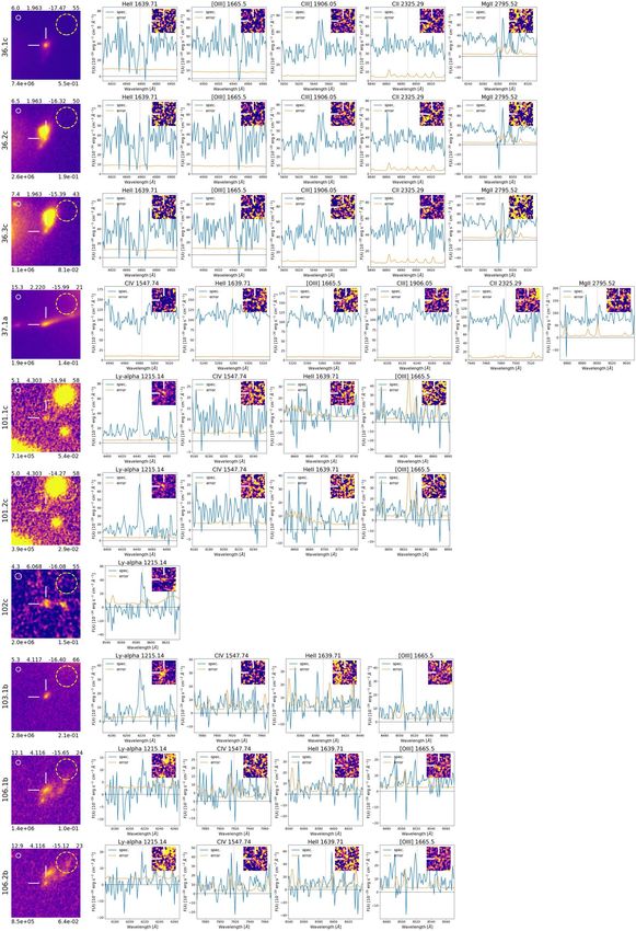
E. Vanzella et al.: Star-forming complexes at cosmological distance

Fig. 8. Examples of MUSE spectra of moderately magnified sources not producing multiple images. In the left panel the one dimensional spectra
are color coded accordingly to the dashed circles marking the sources in the HST color images (middle panels). The spectrum of source 2357
from four hours of integration without AO is compared with the one from the MDLF full depth (17.1 hours) including AO (the P-Cygni profile
of the Civ is affected by the increased noise due to laser AO correction). The deep spectrum shows many features in absorption, whereas in
emission, the Ciii]λλ1907, 1909 and broad Heiiλ1640 (marked with a dashed ellipse) are clearly detected, as well as a possible P-Cygni of the
[NV]λλ1239, 1243, close to the blue edge of the spectral coverage. Two other faint objects, 2046 and -99, are shown with magenta and red
colors. The observed(intrinsic) magnitude is shown in the middle panels, with the intrinsic one reported with a yellow color. Source 2046, with
m1500 = 31.1 ± 0.3, shows a large Lyα equivalent width of 220 ± 25 Å rest-frame and a very steep ultraviolet slope, β = −2.9 ± 0.2. Nebular
Civλ1548, 1550 doublet is also detected for this object (see dashed ellipse on the red spectrum). The rightmost panels show the SED fits and
magnitudes as performed by Castellano et al. (2016). The red spectrum is blueshifted by 12 Å with respect to the other spectra for illustrative
purposes.

ing at HST/ACS and WFC3 images and their RGB color version,              times the Kron radii around each source (see Merlin et al. 2019
in addition to taking into account the mirroring and parity prop-        for details). The figures in Appendix B reveal that such clumps
erties introduced by strong lensing (see Appendix B). The latter         have rather compact sizes, several of them are marginally re-
reinforces the identification of extremely faint clumps (e.g., ob-       solved or entirely unresolved and slightly elongated. The in-
served magnitude > 29 − 30) that are otherwise elusive even for          ferred magnitude can therefore be somewhat affected, however,
deep spectroscopy; this represents a unique advantage provided           we did not apply any correction in this work since our scope
by lensing. Figure 9 shows an example where at least 13 clumps           is focused on the characterization of the new parameter space
associated to source 20 at z = 3.222 are identified, including           opened by these observations – specifically, the size and lumi-
very faint or isolated knots which display in some cases different       nosity at the faint end.
colors (see also source 5, Figure 5). Other examples are shown                Figure 10 shows the observed/intrinsic magnitude distribu-
in Appendix B.                                                           tion of all clumps at z < 4.8 (z > 4.8) extracted from the HFF
     All high-z multiple images have been visually inspected and         HST/F814W (F105W) band, as well as the observed or intrin-
the consistency with their parity properly checked. Among the            sic Lyα fluxes. The absolute magnitude spans the range of [−18,
66 families spanning the redshift range of 1 < z < 6.2, we               −10] with a median of −16, over a redshift range of [1 − 6.7],
identify structured clumps in the majority of the high-z galaxies        with a median of z = 3.5. The distribution of the Lyα fluxes is
(more than 60%). Appendix B describes the sample of clumps,              shown in the same figure. Fluxes were extracted from a fixed
reporting for each of them the HST cutouts and MUSE spec-                aperture of 000. 8 diameter; we did not attempt to tune apertures to
tra. Despite lensing magnification acting to magnify (and distort)       capture the different morphology of the emitting regions, which
galaxies, the identification of clumps is typically not performed        are also shaped by lensing distortion. Unfortunately, the MUSE
by automatic tools of source extraction (e.g., SExtractor pack-          PSF (FWHM=000. 6) prevents us from extracting spectra for the
age, Bertin & Arnouts 1996) since a delicate trade-off between           majority of the clumps, which are blended because of the lower
de-blending and detection threshold segmentation is needed. In-          angular resolution with respect to HST. With this caveat in mind,
deed, the majority of the clumps discussed here are not present          it is worth stressing that for compact Lyα emitters the measured
in the ASTRODEEP (Castellano et al. 2016) or HFF Deep Space              fluxes extend down to a few 10−19 erg s−1 cm−2 , with the faintest
(Shipley et al. 2018) catalogs of HFF J0416. Moreover, the pres-         tail approaching 10−20 erg s−1 cm−2 , as in the case discussed by
ence of bright cluster galaxies in the field makes faint object          Vanzella et al. (2020b) at z = 6.629 straddling the caustic, im-
detection and photometry (contamination) difficult. In order to          plying extremely faint and small sizes of the emitting regions.
characterize their magnitude distribution and homogenize mea-            High-ionization emission lines (typically emerging from much
surements, we made use of the the APHOT tool (Merlin et al.              smaller regions than those producing scattered Lyα, and typi-
2019) and we performed photometric measurements on each of               cally aligned with the HST stellar continuum) are also captured
them over the same images used to build the ASTRODEEP color              at the faintest luminosities in single sources and with high S/N
catalog. To estimate their magnitudes, we adopted 2 × FWHM               ratios on the stacked spectrum, as described in Sect. 5.
diameter apertures and measure their local background through                 An accurate estimate of the size of each object (e.g., the ef-
a sigma clipping procedure in annuli of 10 pixel radius, at 1.2          fective radius) will be part of a future work. Here, we perform a
                                                                                                                  Article number, page 9 of 43
A&A proofs: manuscript no. 39466corr

Fig. 9. Example of a magnified z = 3.222 galaxy (source 20). Deep color RGB images of components 20a and 20c are shown in the two leftmost
panels; the knot showing a redder color with respect to the rest of the galaxy is marked with a green arrow. Cyan arrows mark the two extremes of
the structure, indicating the corresponding physical regions. In the middle panel, the F814W blue color-code HST image details the most magnified
component 20c, in which at least 13 clumps are identified, across a region of 8 physical kpc on the source plane. The contours are drawn from
the MUSE Lyα emission. The MUSE and ACS/F184W PSF sizes are indicated with a red (top-left) and black (bottom-left) circles. The SED-fits
(from the ASTRODEEP photometric catalog, Castellano et al. 2016) of two regions marked with dashed black ellipses are shown in the rightmost
panels. The mirrored symmetry between images 20a and 20c confirms that all clumps belong to the galaxy, including knot 20.0 showing a clearly
different color (see SED fits). The physical scale is reported on image F814W, bottom-right (1 HST pixel corresponds roughly to 60 pc along the
vertical extension of the galaxy in the source plane).

Table 2. Summary of the MDLF observations

   Date                      Quality    OB Name
                             MDLF
   22/23-Nov-2017              A        WFM_J0416_NOAO_1
   10/11-Jan-2018              A        WFM_J0416_NOAO_2
   21/22-Feb-2018              C        WFM_J0416_NOAO_3
   12/13-Mar-2018              X        WFM_J0416_AO_1
   4/5-Nov-2018                A        WFM_J0416_AO_10
   5/6-Nov-2018                B        WFM_J0416_AO_1
   5/6-Nov-2018                A        WFM_J0416_AO_2
   6/7-Nov-2018                A        WFM_J0416_AO_4
   2/3-Dec-2018                A        WFM_J0416_AO_11
   4/5-Dec-2018                A        WFM_J0416_AO_13
   12/13-Dec-2018              A        WFM_J0416_AO_14
   11/12-Jan-2019              B        WFM_J0416_AO_5
   16/17-Jan-2019              C        WFM_J0416_AO_6
   25/26-Jan-2019              A        WFM_J0416_AO_6
   27/28-Feb-2019              A        WFM_J0416_AO_17
   28-Feb/1-Mar-2019           A        WFM_J0416_AO_7
   3/4-Mar-2019                A        WFM_J0416_AO_8
   2/3-Aug-2019                A        WFM_J0416_AO_9
   30/31-Aug-2019              A        WFM_J0416_AO_18                   Fig. 10. Observed (de-lensed) 1500 Å magnitude distributions (top-left)
                              GTO                                         and observed (de-lensed) Lyα flux distribution (top-right) for the sam-
   17-Dec-2014                 A        WFM_J0416_NOAO                    ple of clumps (individual sources). The bottom panels show the absolute
   17-Dec-2014                 A        WFM_J0416_NOAO                    magnitude (left) and redshift (right) distributions. No multiple images
                                                                          are included. The median absolute magnitude of the sample is −16 cor-
Notes. The log of the observed OBs is reported. The typical exposure      responding to an AB magnitude ∼ 30.
time (on sky) of each OB is 3340s. The bottom two rows refer to the
previous 2 hours observation from the GTO. The column “OB Name”
indicates the observing mode ("WFM" = wide field mode) and the use        magnification maps from out new lens model. Clearly this is a
(or not) of the adaptive optics "AO/NOAO," meaning "on/off".              simple assumption and would overestimate the effective radius
                                                                          for compact point-like objects (for which the PSF deconvolution
                                                                          would lead to radii even smaller than the pure PSF, comparable
first analysis by computing the physical size that the HST PSF            to a single HST pixel, e.g., Vanzella et al. 2019). Conversely,
would have if it had been placed at the same locations, using the         it would underestimate the size in the case of extended objects
Article number, page 10 of 43
E. Vanzella et al.: Star-forming complexes at cosmological distance
(see how clumps appear in Appendix B and figures therein). Fig- redshift background sources are contaminated by the intracluster
ure 11 shows the half width at half maximum (HWHM) as a light and by generally red galaxy cluster members, especially in
function of the intrinsic absolute magnitude, redshift, and intrin- the innermost regions of the galaxy cluster. Therefore, spectral
sic magnitude for the whole sample. features due foreground cluster galaxies may remain imprinted
Several clumps appear as faint as (or fainter than) those re- in the final stacked spectrum if not subtracted properly. Second,
ported by Maseda et al. (2018) (or Feltre et al. 2020) from the the presence of multiple images allows us to increase the effec-
MUSE deep observations performed in the Hubble Ultra Deep tive total integration time for a single family. For example, when
Field, where magnitudes 30 − 31 are probed with S/N < 5. In three multiple images with similar levels of magnification (e.g.,
the present case, and not surprisingly, strong lensing allows us to comparable magnitudes) and free from foreground contamina-
probe physical scales out of reach in blank fields (e.g., < 100 tion are available, the total integration time for the single source
pc) and access comparable flux limits with high S/N or even increases to 51.3 hours (17.1 × 3). Naturally, when only one im-
faint sources that have been totally missed in non-lensed fields age is available (for whatever reason), the integration time re-
(e.g., intrinsic magnitude fainter than 31). We note, in fact, that duces to the original integration of 17.1 h for the MDLF (a sim-
several such tiny star-forming regions (e.g., MUV > −16) are ilar argument applies to the SW pointing).
well-detected with S /N > 10, thus allowing a morphological We mitigate the first issue by stacking continuum-subtracted
and SED-fitting analysis even on single sources. As an example, spectra. This procedure implies that we miss the final continuum
a point-like object with an intrinsic magnitude of 29.5 will move slope of the coadded spectrum and it tends to wash out the ab-
down to a magnitude of 26.5 with a magnification of µ = 10; sorption lines as well, even though some signature of absorption
such a magnitude is typically measured with S/N > 20 at the lines still persist (see below). In this section, we focus on the
HFF depth. Similarly, MDLF−like observations will probe emis- detection of emission lines.
sion lines at unprecedented faint flux levels (see Sect. 5). We adopted the following strategy to compute the stacked
In order to highlight the gain provided by strong lensing, Fig- spectrum: (1) For spectra in the redshift range of 1.7 <
ure 11 also includes a sample of galaxies extracted from non- z < 3.9, the Ciii]λλ1907, 1909 line wavelength is captured by
lensed fields at 3.5 < z < 6.5 (from the GOODS-South, Vanzella MUSE. The systemic redshifts have been measured from at
et al. 2009; Giavalisco et al. 2004). High-z galaxies studied in least one of the following nebular high-ionization emission lines:
non-lensed fields have typical sizes of kpc (or sub-kpc) scale Civλ1548, 1550, Heiiλ1640, Oiii]λ1661, 1666, and Ciii]λ1908,
and magnitudes typically brighter than MUV = −18. In lensed which often are detected on individual spectra (as also the me-
fields and in this work, the same class of sources can be de- dian stacked spectrum demonstrates, see below). The redshift
composed into clumps of 100-200 pc size at typical magnitude from the Lyα line is used if no other lines are present. Here,
MUV = −16 as the angular resolution increases. These clumps we decided to exclude the sample at z > 3.9, for which the high-
includes the most extreme cases for which single star clusters ionization lines mainly lie in the forest of sky emission lines.
can be probed, down to MUV = −15 with sizes smaller than 50 (2) Each one-dimensional spectrum is continuum-subtracted by
parsec (e.g., Zick et al. 2020; Bouwens et al. 2017b; Kawamata using a smoothing-spline and successively weighted by the
et al. 2015), including globular cluster precursors (Vanzella et al. inverse of the corresponding error spectrum provided by the
2017b, 2019). Concerning the very faint-end of the magnitude- MUSE pipeline. The resulting continuum-subtracted S/N spec-
size distribution, sources that are barely detected − even when tra have more regular sky residuals and can be considered as
assisted by lensing magnification − correspond to intrinsic mag- S/N detection maps. The measurements of line ratios are, how-
nitudes in the range of 33 − 35, with extreme cases even fainter ever, performed on the continuum-subtracted stack. (3) Spec-
than 35 (Vanzella et al. 2020b). It is worth stressing that un- tra belonging to multiple images of the same family have been
resolved objects (smaller than 40 − 50 pc) showing prominent combined by computing a weighted average, where the weights
Lyα emission at z = 3.5 and suggesting a high ionization field are assigned after a visual inspection of each multiple image,
provided by young stellar populations, with magnitudes fainter based on the observed magnitudes, the magnifications factors,
than m1500 = 31 (MUV = −14.8), correspond to stellar masses of and presence of possible contaminants (e.g., by excluding the
. 106 M in the instantaneous burst assumption and are weakly cases outshone by nearby foreground objects).
dependent on metallicity or IMF (Leitherer et al. 2014). Irrespec- In this way, we selected 61 (out of 66) individual objects,
tive of the nature of such objects, they are more likely to belong excluding five of them due to redundant information – namely,
to the realm of star forming complexes or even massive star clus- close clumps that are undistinguished by the MUSE extraction
ters with MUV = −13 or fainter (Atek et al. 2015; Alavi et al. aperture of 000. 8 in diameter and that would enter more than
2014, 2016; Atek et al. 2018; Bouwens et al. 2017b; Livermore one time in the stacking); 33 out of 61 satisfy the condition
et al. 2017). Thus, the current demography of the faint-end of 1.7 < z < 3.9. The average weighted exposure time for the 61
the ultraviolet luminosity functions of “high-z galaxies” may be objects is 33 hours (ranging between 17.1 to 51.3 hours) and
contaminated or even perhaps dominated by these low-mass star the equivalent total weighted integration time for the stacked
systems (Pozzetti et al. 2019; Boylan-Kolchin 2018; Elmegreen spectrum in the wavelength range of Lyα− Ciii]λ1908 spans be-
et al. 2012), implying that the term “galaxy” for this class of faint tween 600 to 1000 hours, without including the amplification µ.
sources does not seem appropriate. By adopting an average µ = 4, the equivalent integration time
needed to obtain a similar depth in unlensed fields would add up
to & 10000 hours.
5. Spectral stacking and high-ionization nebular Figure 12 illustrates the stacking steps. The raw
lines detected on individual sources to mean/median stack without continuum subtraction is shown in
MUV ∼ −16 panel A, highlighting the smooth red pattern emerging from
the foreground cluster contamination. The mean/median stack
Before discussing the method used to coadd spectra from a set of continuum subtracted spectra is reported in panel B. The
of sources, it is worth mentioning two main differences between S/N detection map obtained after inversely weighting each
lensed and non-lensed fields. First, in lensed fields, the high- continuum-subtracted spectrum by its error spectrum is shown
Article number, page 11 of 43You can also read