CACTI Radar b1 Processing: Corrections, Calibrations, and Processing Report - DOE/SC-ARM-TR-244 - Atmospheric Radiation ...
←
→
Page content transcription
If your browser does not render page correctly, please read the page content below
DOE/SC-ARM-TR-244

CACTI Radar b1 Processing: Corrections,
Calibrations, and Processing Report

JC Hardin     A Hunzinger
E Schuman     A Matthews
N Bharadwaj   A Varble
K Johnson     S Giangrande

May 2020
DISCLAIMER

This report was prepared as an account of work sponsored by the U.S.
Government. Neither the United States nor any agency thereof, nor any of
their employees, makes any warranty, express or implied, or assumes any
legal liability or responsibility for the accuracy, completeness, or
usefulness of any information, apparatus, product, or process disclosed, or
represents that its use would not infringe privately owned rights. Reference
herein to any specific commercial product, process, or service by trade
name, trademark, manufacturer, or otherwise, does not necessarily
constitute or imply its endorsement, recommendation, or favoring by the
U.S. Government or any agency thereof. The views and opinions of
authors expressed herein do not necessarily state or reflect those of the
U.S. Government or any agency thereof.
DOE/SC-ARM-TR-244

CACTI Radar b1 Processing: Corrections,
Calibrations, and Processing Report

JC Hardin, Pacific Northwest National Laboratory (PNNL)
A Hunzinger, PNNL
E Schuman, PNNL
A Matthews, PNNL
N Bharadwaj, PNNL
A Varble, PNNL
K Johnson, Brookhaven National Laboratory (BNL)
S Giangrande, BNL

May 2020

Work supported by the U.S. Department of Energy,
Office of Science, Office of Biological and Environmental Research
JC Hardin et al., May 2020, DOE/SC-ARM-TR-244

            Acronyms and Abbreviations
ADI      ARM Data Integrator
AMF      ARM Mobile Facility
ARM      Atmospheric Radiation Measurement
BNL      Brookhaven National Laboratory
CACTI    Cloud, Aerosol, and Complex Terrain Interactions
CSAPR2   C-Band Scanning ARM Precipitation Radar 2
COR      Sierras de Córdoba
CSU      Colorado State University
DOD      data object definition
DOE      U.S. Department of Energy
eRCA     extended relative calibration adjustment
FIR      finite impulse response
GPM      Global Precipitation Measurement satellite (NASA)
HPC      high-performance computing
HSRHI    hemispherical range height indicator
IOP      intensive observational period
KASACR   Ka-Band Scanning ARM Cloud Radar
KAZR     Ka Zenith ARM Radar
KDP      specific differential phase
NASA     National Aeronautics and Space Administration
netCDF   Network Common Data Form
OMT      orthomode transducer
PI       principal investigator
PNNL     Pacific Northwest National Laboratory
PPI      plan position indicator
RCA      relative calibration adjustment
RCS      radar cross-section
RF       radio frequency
RH       relative humidity
RHI      range height indicator
SNR      signal-to-noise ratio
UTC      Coordinated Universal Time
VAP      value-added product
XSACR    X-Band Scanning ARM Cloud Radar
ZDR      differential reflectivity factor
ZPPI     zenith plan position indicator

                                     iii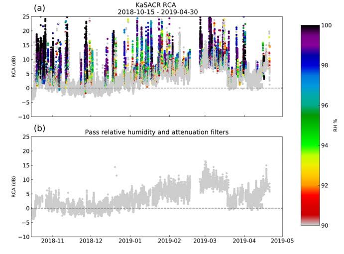
JC Hardin et al., May 2020, DOE/SC-ARM-TR-244

                                                                   Contents
Acronyms and Abbreviations ...................................................................................................................... iii
1.0 Introduction .......................................................................................................................................... 1
       1.1 Overview of CACTI ..................................................................................................................... 1
       1.2 CACTI Radar Assets .................................................................................................................... 2
       1.3 b1 Processing ............................................................................................................................... 2
           1.3.1 Calibration ......................................................................................................................... 3
               1.3.2 Data Quality Masks ........................................................................................................... 3
               1.3.3 Data Quality Corrections ................................................................................................... 4
           1.3.4 Derived Fields ................................................................................................................... 4
       1.4 Radar Performance ....................................................................................................................... 4
       1.5 Scan Strategy ................................................................................................................................ 5
               1.5.1 Standard Scan Strategy...................................................................................................... 6
               1.5.2 Agile Scanning .................................................................................................................. 6
               1.5.3 Phase Two Scanning ......................................................................................................... 6
2.0 Calibrations and Corrections ................................................................................................................ 7
       2.1 Techniques ................................................................................................................................... 7
               2.1.1 Corner Reflector Calibration ............................................................................................. 7
               2.1.2 Relative Calibration Adjustment ....................................................................................... 8
               2.1.3 Self-Consistency................................................................................................................ 9
               2.1.4 Differential Cross-Calibration ......................................................................................... 10
           2.1.5 Differential Reflectivity (ZDR) Correction ....................................................................... 12
       2.2 CSAPR2 Calibrations and Corrections ...................................................................................... 12
               2.2.1 Reflectivity (Z) Correction .............................................................................................. 12
               2.2.2 Differential Reflectivity (ZDR) Correction ....................................................................... 14
       2.3 XSACR Calibrations and Corrections........................................................................................ 16
               2.3.1 Radar Constant Correction .............................................................................................. 16
               2.3.2 Reflectivity (Z) Correction .............................................................................................. 17
           2.3.3 Differential Reflectivity (ZDR) Correction ....................................................................... 20
       2.4 KASACR Calibrations and Corrections ..................................................................................... 22
               2.4.1 Waveguide Blockage Correction..................................................................................... 22
               2.4.2 Reflectivity (Z) Correction .............................................................................................. 23
       2.5 KAZR Correction ....................................................................................................................... 27
               2.5.1 Cross-Comparisons with KASACR ................................................................................ 27
               2.5.2 KACR Intermode Comparison ........................................................................................ 29
3.0 Masks .................................................................................................................................................. 30
       3.1 CSAPR2 Masks .......................................................................................................................... 30

                                                                              iv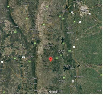
JC Hardin et al., May 2020, DOE/SC-ARM-TR-244

       3.2 XSACR Masks ........................................................................................................................... 31
       3.3 KASACR Masks ........................................................................................................................ 31
4.0 Derived Fields..................................................................................................................................... 32
       4.1 Specific Differential Phase (KDP) ............................................................................................... 32
       4.2 Attenuation Correction ............................................................................................................... 32
5.0 Processing Architecture ...................................................................................................................... 35
       5.1 Overall Architecture ................................................................................................................... 36
       5.2 Plug-In-Based Architecture ........................................................................................................ 36
       5.3 Corrections Configuration Files ................................................................................................. 38
               5.3.1 Configuration Index File ................................................................................................. 38
               5.3.2 Processing Configuration File ......................................................................................... 39
       5.4 Data Provenance......................................................................................................................... 41
       5.5 Parallel Processing ..................................................................................................................... 42
       5.6 Impact of New Processing System ............................................................................................. 42
       5.7 Available Plug-Ins ...................................................................................................................... 42
6.0 Description of Data Files .................................................................................................................... 43
7.0 References .......................................................................................................................................... 45

                                                                        Figures
1     DOE ARM CACTI site in Argentina outside Villa Yacanto. ................................................................ 1
2     Radars installed at AMF1 site for CACTI. ............................................................................................. 2
3     Radar b1 computational flow graph. ...................................................................................................... 3
4     Timeline of CACTI radars operating status during the campaign, 15 October 2018−30 April
      2019. ....................................................................................................................................................... 5
5     Scan strategy prior to CSAPR2 motor failure. ....................................................................................... 6
6     Phase two radar scan strategy, valid from around 2 March, 2019 through end of campaign. ................ 7
7     Corner reflector calibration from raster scans. Panel (a) is the scan without the corner reflector
      installed. (b) is the result with the corner reflector installed, but blockage in the waveguide. (c) is
      with the blockage removed..................................................................................................................... 8
8     ΦDP reconstruction for self-consistency calibration. ............................................................................. 10
9     CSAPR2 daily median RCA values calculated during the CACTI field campaign. ............................ 13
10 HSRHI clutter map generated from CSAPR2 using the composite clutter map method in (5). .......... 13
11 CSAPR2 daily median RCA during the CACTI field campaign using a1-level data files and b1-
   level data files. ...................................................................................................................................... 14
12 Daily median ZDR (black dots) for CSAPR2 during CACTI. ............................................................... 15
13 CSAPR2 daily median a1 ZDR (black) with offwets (blue) and daily median b1 ZDR (green). ............ 15
14 HSRHI of CASPR2 before and after various corrective steps. ............................................................ 16

                                                                                 v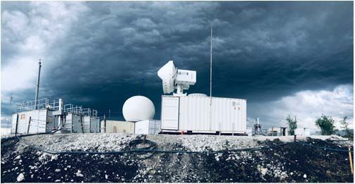
JC Hardin et al., May 2020, DOE/SC-ARM-TR-244

15 (a) XSACR daily median RCA (gray) during CACTI before the discovery of a changing radar
   constant................................................................................................................................................. 17
16 HSRHI clutter map generated for XSACR during CACTI using the composite clutter map
   method described in (5). ....................................................................................................................... 18
17 Daily median RCA using a1-level XSACR data (gray) and b1-level XSACR data (blue). ................. 18
18 Reflectivity cross-comparisons between XSACR and CSAPR2 at the COR CACTI site. .................. 19
19 Distribution of reflectivity cross-comparison differences between XSACR and CSAPR2 using
   b1-level data during November and December 2018. .......................................................................... 20
20 Weekly median ZDR with offsets calculated using a1-level XSACR ZDR (dots), weekly median
   b1-level ZDR (squares) and daily media b1-level XSACR ZDR (triangles), colored by standard
   deviation (must be less than 1). ............................................................................................................ 21
21 Weekly median ZDR for XSACR during CACTI colored by standard deviation less than 1. .............. 21
22 Sample HSRHIs from XSACR from (top) a1 Z and ZDR, (middle) b1 Z and ZDR, and (bottom) b1
   attenuation corrected Z and ZDR. .......................................................................................................... 22
23 Debris removed from KASACR waveguide. ....................................................................................... 23
24 HSRHI clutter map generated for KASACR during CACTI using the composite clutter map
   method in (5). ....................................................................................................................................... 23
25 KASACR daily median RCA values calculated during the CACTI field campaign............................ 24
26 Daily median RCA values for KASACR using a1-level data (red) and b1-level data (blue). ............. 24
27 Sub-daily KASACR RCA values (pink and navy) from a1-level data, relative humidity (RH)
   values from surface statin (RH90 in green), rain rates from Pluvio data
   (blue), reflectivity difference between X/KASACR (black). ............................................................... 25
28 (a) Sub-daily KASACR RCA during full CACTI campaign, colored by relative humidity (RH)
   greater than 90%. (b) Sub-daily KASACR RCA that pass attenuation filtering and times when
   RH
JC Hardin et al., May 2020, DOE/SC-ARM-TR-244

                                                                       Tables
1    Radar specifications during the CACTI field campaign. ....................................................................... 5
2    Ranges and thresholds used for gate selection during reflectivity cross-comparisons between
     radars. ................................................................................................................................................... 11
3    Attenuation coefficients (a,b) used for calculating specific attenuation for each radar. ...................... 11
4    Censor map (CMAP) bitfield definitions. ............................................................................................ 31
5    Classification Mask for CSAPR2 bitfield definitions. ......................................................................... 31
6    Coefficients used to calculate specific attenuation, AH = α KDPcin b1 processing. ............................. 33
7    Available plug-ins. ............................................................................................................................... 42
8    CSAPR2 file contents. .......................................................................................................................... 43
9    XSACR file contents. ........................................................................................................................... 44
10 KASACR file contents. ........................................................................................................................ 45
11 KAZR file contents. ............................................................................................................................. 45

                                                                              vii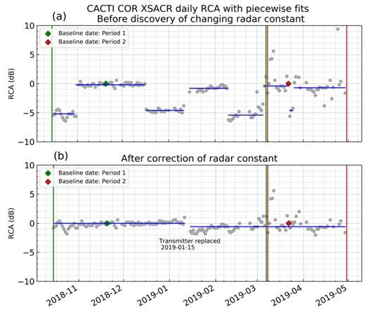
JC Hardin et al., May 2020, DOE/SC-ARM-TR-244

1.0    Introduction
 The U.S. Department of Energy’s (DOE) Atmospheric Radiation Measurement (ARM) user facility
 deployed a large number of instruments to a region nearby the Sierra de Córdobas mountains in Argentina
 as part of the Cloud, Aerosol, and Complex Terrain Interactions (CACTI) field campaign (1). During this
 campaign, four radars were installed at a site outside of Villa Yacanto as shown in Figure 1. As part of a
 post-campaign effort to improve the usability of these data, a significant activity was undertaken towards
 the calibration, correction, and improvement of the data quality of these radar datastreams.

                   Figure 1.    DOE ARM CACTI site in Argentina outside Villa Yacanto.

 This process in ARM nomenclature is referred to as generating a “b1” datastream. While these “b1”
 standards may imply different corrections or standards for various ARM instruments, for radars it refers
 to a datastream that has been calibrated (and cross-calibrated), including a serious effort to deliver the
 highest-quality (well-characterized) data possible. This report details (i) the status/quality of the original
 “a1” (raw) data, (ii) the corrections and calibrations that are applied to generate these b1 datastreams,
 (iii) the details of the applied algorithms and how radar offset/calibration numbers were determined for
 the eventual corrections, and (iv) the new and flexible plug-in-based processing system designed during
 CACTI for radar b1 activities (current, future) that interfaces with ARM’s Data Integrator (ADI) and
 high-performance computing (HPC) system.

 1.1 Overview of CACTI
 The CACTI field campaign was “designed to improve understanding of cloud life cycle and organization
 in relation to environmental conditions so that cumulus, microphysics, and aerosol parameterizations in
 multiscale models can be improved.”(1) The location was chosen in large part due to the frequent
 initiation and development of convective storms off the nearby ridgelines. This frequency of convective

                                                        1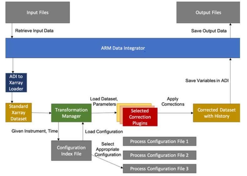
JC Hardin et al., May 2020, DOE/SC-ARM-TR-244

initiation makes it practical to capture a large number of storms with a stationary site. The CACTI
campaign did not disappoint and sampled a very large number of target cases including more than 100
convective days. As such, the frequency of convection provides a very target-rich data set well suited to
the benefits that follow the often time-consuming and labor-intensive efforts required to ensure good
calibration and data quality.

1.2 CACTI Radar Assets
Four radars were deployed to CACTI. These included (i,ii) the Ka-Band Scanning ARM Cloud Radar
(KASACR) and the X-Band Scanning ARM Cloud Radar (XSACR), a co-mounted, dual-frequency
system, (iii) the Ka ARM Zenith Radar (KAZR; a zenith-pointing profiling radar), and (iv) the first
deployment of the C-Band Scanning ARM Precipitation Radar 2 (CSAPR2). All radars were installed at
the main first ARM Mobile Facility (AMF1) site (labeled COR:M1), as shown in Figure 2. The
specifications for the radars are found in Table 1.

                           Figure 2.    Radars installed at AMF1 site for CACTI.

1.3 b1 Processing
It is important to differentiate the algorithms included in b1 processing, and what activities/scope are
reserved for downstream value-added products (VAPs) or other user-supported processing (e.g., c1-level,
or principal investigator [PI] products). At the outset, several limiting boundaries on b1 processing were
established. Overall, the first and most significant limitation is that these processing efforts are restricted
to activities constrained by a single instrument. That is, although b1 efforts may consult or perform
comparisons against other instruments to obtain information about the corrections for an individual b1
datastream, there is no merging of separate ARM datastreams and/or uses of other instruments at
processing time.

There are several different steps in the b1 processing chain. This section covers each of these steps at a
high level, before describing various steps in additional detail in the remaining sections of this document.
The general flowchart of b1 efforts can be seen in Figure 3.

                                                       2
JC Hardin et al., May 2020, DOE/SC-ARM-TR-244
Figure 3. Radar b1 computational flow graph.
1.3.1 Calibration
The primary purpose of the b1 processing is the calibration of the radar datastreams. As will be shown in
future sections, there are a variety of ways in which the calibration of a radar can drift. The primary
function of calibration is to fix the value of the radar constant C. This constant affects nearly all power
measurements the radar takes and represents one of the most dominant sources of errors for the radar.
Fundamentally the radar constant is used as
The radar constant C itself is made up of numerous terms including the finite filter loss, the gain of the
antenna, the wavelength, and many others. We can, however, represent it as a constant and, once solved
for, correcting calibration is a linear operation for a given time step. This calibration constant exists for
both polarizations (where polarization is used) and has a unique value for each. In the case of the KAZR,
where pulse compression is used, this has additional terms based on the pulse compression gain. As such,
we need to solve for numerous radar constants for each radar. This calculation is also not necessarily
constant in time (on longer time scales), as the transmitted power of the radar, the waveguide loss, and
many other factors may drift with changes in the environment and radar stability.
For the calibration of the CACTI radars, we have used a wide variety of existing techniques, as well as
implemented several new options. These options enable a more robust measure of radar calibration/offset
than has been provided for previous ARM campaigns. Additionally, these efforts have heavily used
cross-calibration checks with all radars on site and to other-agency partner radars in the area. These ideas
extend to satellite overpass concepts, that also help ensure as good a calibration as possible.
1.3.2 Data Quality Masks
The radar measures not only hydrometeors in the atmosphere, but also insects, ground clutter, and
extraneous radio frequency (RF) interference. To make the most use of these data, it is useful to construct
a series of masks to isolate individual fault conditions in the data. These serve as an index of when data
are good or bad, depending on the usage. For instance, a common mask is insects − this is not necessarily
an indication of bad data if the user goal is to study clear-air/wind, as insects are often passive tracers of
the air motion. Therefore, the application of these masks often depends upon the usage for which they are
intended. Because the processing and measured parameters change for each radar, the masks available for
individual datastreams will vary from radar to radar.
3JC Hardin et al., May 2020, DOE/SC-ARM-TR-244
1.3.3 Data Quality Corrections
In addition to calibration and data quality masks, sometimes there are larger events or circumstances that
cause the radar data to be bad/poor. Sometimes, these issues (e.g., complete power/site outage) are not
correctable, but in some instances these issues can be remedied. Wherever possible, we attempt to correct
for malfunctions or misconfigurations on the radar. For instance, the XSACR during CACTI had a
periodic change in the radar constant due to an improperly specified configuration file. These efforts have
corrected for these types of issues as much as possible within current resources. When a correction could
not be provided, we will attempt to note it in this report.
1.3.4 Derived Fields
To facilitate downstream processing such as VAP and PI product development, it was requested that these
b1 efforts include basic derived products within these data. In particular, for the radars that have
polarimetry, one addition was to estimate the specific differential phase (KDP) and provide basic
corrections for attenuation in rain. Specific differential phase KDP in particular is useful for a wide
variety of downstream products, as well as for improved interpretation of the data itself. Attenuation
correction in rain provides a measure of the power lost to the environment as the beam propagates
through hydrometeors. The efforts have elected to implement simple, well-tested algorithms over
potentially better, but less stable, implementations. These fields are not intended to be the best/end
estimate for all radar data users but provide a baseline/reference estimate suitable for initial product
development. Some users and VAP authors may elect to process these data with more sophisticated
techniques, which may be recommended for advanced applications in deep convective cores at shorter
radar wavelengths – as common to the CACTI data set.
1.4 Radar Performance
CACTI was a very successful campaign for ARM in terms of radar performance and uptime. This is
partially attributed to the conditioning and preparation period for these radar at the Pacific Northwest
National Laboratory (PNNL) before the campaign started − where a large number of systems were
analyzed, replaced, or upgraded if needed. Thus, the radars were able to capture data over the entire
campaign, in a generally good state. Shown in Figure 4 is the uptime of the radars during CACTI (where
the radar is considered “up” if data were produced at any time during that day).
4JC Hardin et al., May 2020, DOE/SC-ARM-TR-244
Figure 4. Timeline of CACTI radars operating status during the campaign, 15 October 2018−30 April
2019.
However, during the campaign, the radars did encounter various issues causing periodic downtime, as
shown in red in Figure 4. There was downtime for the CSAPR2 around the turn of the year, resulting in a
period of no data. Beginning in February, there were additional issues with the pedestal on the CSAPR2.
Ultimately, this resulted in failure for the ability to scan this radar in azimuth. As a result, campaign PIs
and ARM redesigned CSAPR2 scan strategies to include plan position indicator (PPI) scans on the
Scanning ARM Cloud Radar (SACR), while performing a single azimuth range height indicator (RHI)
scan with a very high update rate (45 seconds) on the CSAPR2. The period with modified scan strategies
is denoted in yellow in Figure 4.
Table 1. Radar specifications during the CACTI field campaign.
Transmit Antenna Beam Gate
Frequency Wavelength power diameter width spacing
Radar (GHz) (cm) (kW) (m) (deg) (m) Polarization
CSAPR2 5.7 5.26 350 4.3 0.9 100 Dual
XSACR 9.71 3.09 20 1.82 1.4 25, 75 Dual
KaSACR 35.3 0.85 2 1.82 0.33 25 Horizontal
KAZR 34 0.857 0.187 2 0.3 29.98 Single
1.5 Scan Strategy
Due to changes in operational strategy, and failures in the pedestal on the CSAPR2 as introduced above,
three distinct scan strategies were used during the campaign.
5JC Hardin et al., May 2020, DOE/SC-ARM-TR-244
1.5.1 Standard Scan Strategy
The radar scan strategy for CACTI was designed to maximize the capture of convective initiation, while
still providing high-resolution scans in the vertical dimensions as storms pass over the site. Figure 5
shows the original scan strategy for the first months of the campaign. The CSAPR2 is designed to provide
spatial context with PPI scans, before transitioning to a zenith PPI (ZPPI) for a vertical profile (and
differential reflectivity factor [ZDR] calibration), and then moving to two sets of hemispherical range
height indicator (HSRHI) scans that start at 0 degrees azimuth and occur at every 30 degrees in azimuth
until the entire domain has been covered. These HSRHI scans correspond to an angular positioning of (0,
30, 60, 90, 120, 150). Due to the hemispherical nature of the scans, this implies an entire 360-degree area
is sampled with those six slices.
The KA/XSACR scanning was designed to provide more vertical information/structure for the convective
clouds and thus consisted of an RHI sector, followed by three sets of HSRHIs with similar
coverage/design as those implemented for the CSAPR2. The scans were also designed to overlap
temporally during these HSRHI modes as much as possible through their implementations.
Figure 5. Scan strategy prior to CSAPR2 motor failure. During agile scanning the CSAPR2 HSRHIs
are replaced by agile RHIs. This scan strategy was valid from the start of the campaign until
about 2 March 2019.
1.5.2 Agile Scanning
During the IOP, occasionally there was a decision to elect to place radars into an “agile scanning” mode,
in consultation with the PI/science team for the CSAPR2. During these periods, the radars would switch
to a custom-developed scan controller with a command line interface, as well as a custom scan strategy.
This scan strategy replaces the 2 HSRHIs with a RHI stack controlled by the operator. The custom
controller interface allows the operator to set a few variables (center of scan, scan height, RHI spacing
width) and the rest of the parameters are automatically controlled by the system. Therefore, the RHIs
during this period can (and will) change from time to time. Otherwise all b1 processing is identical for
this period.
1.5.3 Phase Two Scanning
Due to a failure in the azimuth servo motor on the CSAPR2 in late February, the scanning strategies of
the radars were reworked. The CSAPR2 was set to a “fast RHI” mode, directed along the 270-degree
azimuth, with 45-second heartbeat. This choice was due to CSAPR2 inability to rotate in azimuth. To
6JC Hardin et al., May 2020, DOE/SC-ARM-TR-244
maintain a sense of what was happening spatially, a 15-tilt PPI was added to the KA/XSACR while the
range was increased to 60 for the XSACR. To keep the heartbeat, this necessitated removing the
KA/XSACR RHI sector scan mode, as well as removing one of the HSRHI scan types. The new scan
strategy is shown in Figure 6.
Figure 6. Phase two radar scan strategy, valid from around 2 March 2019 through end of campaign.
2.0 Calibrations and Corrections
Under normal conditions, the calibration of the radars is a multi-part process that consists of several tasks
including onsite measurements of transmit power, receiver calibration, and many other tasks. These
efforts are typically complemented by a series of calibration scans as partially introduced in previous
sections, including birdbath (e.g., ZPPI), scans of a corner reflector, and additional cross-comparisons to
ARM and partner radars. Unfortunately, owing to an issue with customs and shipping, the primary
calibration equipment for the radar did not arrive on site. In consequence, there was no ability to perform
an absolute calibration with RF test equipment.
Due to this limitation, radar calibration had to be based on a series of relative calibrations. This section
details the idea behind each measurement/experiment and how it informs the eventual calibration − before
presenting the results/summary for these ideas and how they result in the final b1 calibration. Results of
this section are fed into the plug-in-based processing system detailed in Section 5.0 and used to process
these radar data.
2.1 Techniques
Several techniques are used to calibrate and correct reflectivity-based variables, such as reflectivity and
differential reflectivity, for the CACTI radars. The following subsections describe the techniques and how
they are applied to the radars.
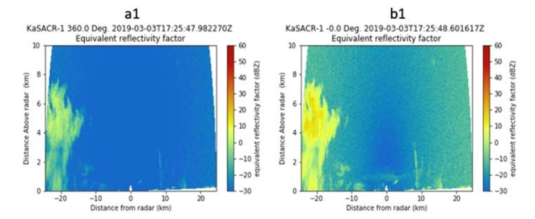
2.1.1 Corner Reflector Calibration
While many onsite RF measurements are normally done, there is inevitably a portion of the RF chain
(nominally, the antenna) that we are unable to calibrate on site. The corner reflector calibration is one
method we use to do an end-to-end calibration. Given the transmit power of the radar (which we can
measure), we bounce a signal off of an elevated trihedral reflector a distance from the radar. This reflector
7JC Hardin et al., May 2020, DOE/SC-ARM-TR-244
has a known radar cross-section (RCS), so we know how much power is expected back at the radar from
this reflector. An example of this procedure is detailed in (2). Trihedral corner reflectors are used because
of their relative insensitivity to pointing errors. For a trihedral corner reflector with edge length l, we can
calculate the maximum RCS as
A host of practical issues are known for corner reflector calibrations. For example, these efforts require
reconfiguring the signal processor and transmit chain, as well as special processing. In the absence of
some of these changes, the error in the corner reflector estimates can be large. In the case of CACTI,
corner reflector calibration was performed towards the end of the campaign, but due to the method
applied for this processing, the effort resulted in an offset/calibration number that was off by 4 dB based
on the analysis on the following sections. This is obviously not adequate for calibration.
These efforts, although not adequate for calibration, did initially point to a significant issue in the
KASACR data sets. Moreover, this initial result from the KASACR was much different than expected.
After having site operations go through the system, we discovered a blockage had built up in the
waveguide. After removal, the numbers matched up better, although still with a 4-dB error that was only
discovered much later in post-processing. While this was a useful activity, and one of the few ways ARM
has to check calibration end to end, these concepts ultimately proved to be less useful for the CACTI field
campaign in terms of establishing b1 calibrations.
Figure 7. Corner reflector calibration from raster scans. Panel (a) is the scan without the corner
reflector installed. (b) is the result with the corner reflector installed, but blockage in the
waveguide. (c) is with the blockage removed.
2.1.2 Relative Calibration Adjustment
Even for campaigns featuring viable corner reflector efforts, a proper radar calibration is recommended to
provide an operational, online mechanism to monitor the calibration/offsets during the course of the
campaign. Previous work in the field (3, 4) has shown that the clutter around a radar can be used as a
relative calibration target. This technique, relative calibration adjustment (RCA), does not calibrate the
radar directly, but rather monitors how drifts in calibration occur in time. For a complete calibration
effort, one can often combine “absolute type” calibrations interwoven with multiple relative calibrations
to inform on radar data quality over extended periods. Such combined efforts have not, however, been
8JC Hardin et al., May 2020, DOE/SC-ARM-TR-244
validated for higher-frequency (above C-band) radars. As part of these CACTI efforts, ARM activities
extended such RCA techniques up through Ka-band radars (5).
One restriction of the previous uses for RCA techniques is that it was initially applied/applicable on PPI
modes, which were not available from the SACRs until the end of the CACTI campaign. As part of the
current work, additional efforts were performed to extend these techniques to overcome this limitation
and allow them to work with RHIs. This new extended RCA (eRCA) technique will form the foundation
on which much of this calibration rests. The details of the technique can be found in (5). The technique
works by establishing a baseline value on a given day, and then all values are relative to this baseline
value.
To interpret the RCA implications on calibration monitoring, one may consider the sign of the RCA
value. For example, an RCA greater than zero means that the daily value is less than the baseline value, or
the radar is running “cold”. RCA less than zero means the daily value is greater than the baseline value, or
the radar is running “hot”. The values are a direct adjustment, which means that by adding the RCA value
back into the reflectivity field, you have matched the calibration of that day to the baseline day.
2.1.3 Self-Consistency
After discussions with an outside research group (Dr. Chandrasekar at Colorado State University [CSU])
that performed a comparison of CSAPR2 to the Global Precipitation Measurement (GPM) satellite, it was
suggested that the calibration error may be different than was indicated by the initial corner reflector
scans. The GPM comparison, however, was only done at one period during the campaign and requires
some subtlety to accomplish. We therefore wanted a technique to “break the tie” between the corner
reflector and the GPM overpass comparison.
Without the corner reflector as an absolute calibration target, we were forced to look elsewhere for a way
to tie the relative adjustments from RCA and cross-comparisons to a single calibration point. One method
used in the past has been to compare with a disdrometer, but as the disdrometer for CACTI was
co-located with the instruments, this comparison becomes somewhat more difficult and less reliable. One
other method that has been used to some success in other projects has been to tie the results of calibration
to the internal self-consistency of the dual-polarization measurements (6). This method is not particularly
robust and relies on some interpretation (choice of filters) and so is not our first choice but is necessary to
determine whether the corner reflector or the single GPM overpass was correct. There are better
implementations (namely areal averaging) of this technique, but we elected to go with a simple
implementation here just to “break the tie” between the two previous methods.
The self-consistency technique works on the principle that triplets of reflectivity, differential reflectivity,
and KDP live in some space that is less than three-dimensional. As such, one can reconstruct one variable
based on the other two to some accuracy. Most commonly, this takes the form of calculating FDP along a
profile based on reflectivity and differential reflectivity. Then, by comparing the measured FDP profile,
and the reconstructed FDP profile, one can determine calibration accuracy.
Ultimately the result of this process confirmed the GPM result (of ~2 dB) for the CSAPR2.
One of the requirements for this technique is a well-calibrated differential reflectivity and differential
attenuation correction. In the case here we only chose leading edges of clouds to avoid attenuation and
9JC Hardin et al., May 2020, DOE/SC-ARM-TR-244
differential attenuation. This is much easier to accomplish and is shown in Section 2.1.5. As mentioned
previously, this is not the most robust technique as implemented here, and we would otherwise not have
elected to use it except where we have the secondary comparison with GPM. An example of the
reconstruction can be seen in Figure 8.
Figure 8. ΦDP reconstruction for self-consistency calibration.
2.1.4 Differential Cross-Calibration
Having confidence in a strong set of 'relative’ calibration checks for the CSAPR2 at a point in time (GPM
and self-consistency) as a ‘absolute’ reference, and a way of tracking calibration changes (eRCA), we can
then use the CSAPR2 to start calibrating the other radars. This effort takes some care, as the radars are
different frequencies, and therefore the measurements of the same target are still expected to differ, even
in the case of perfect calibrations.
Differential (cross-radar) calibration requires radar gates from different radars to be matched in space and
time to ensure similar precipitation is compared. Co-mounted and co-located radars at the CACTI Sierras
de Córdoba (COR) site allowed for reflectivity cross-comparisons. Synchronized scan strategies were
designed and implemented to provide as much temporal overlap as possible. Comparisons were
performed between CSAPR2 and XSACR, and XSACR and KASACR. Given the varying gate spacing
and beam widths of the three radars (see Table 1 for radar specifications), the radar with the smaller beam
width and gate spacing is matched to the nearest azimuth, elevation, and range of the radar with the larger
beam width and gate spacing. Once radar gates are matched, we filter for conditions of light precipitation.
Light precipitation is defined to be low reflectivity (ZH < 15 or 25 dBZ depending on the pair as seen in
10JC Hardin et al., May 2020, DOE/SC-ARM-TR-244
Table 2) and meteorological correlation coefficient (ρhv > 0.95). See Table 2 for radar-specific rejection
criteria thresholds used for differential cross-calibrations.
Table 2. Ranges and thresholds used for gate selection during reflectivity cross-comparisons between
radars.
Radar band comparison Reflectivity Correlation Elevation Path-integrated
range (ZH, dBZ) coefficient minimum range attenuation
(ρhv) (deg) maximum
(IAH, deg km-1)
X-C -5, 25 0.95 10 - 170 0.1
X - Ka -5, 15 0.95 10 - 170 0.1
Radar attenuation in rain is a concern for higher-frequency radars, especially when observing heavy rains
and severe weather. We performed path-integrated attenuation filtering on XSACR and KASACR.
Specific attenuation, AH, was calculated using a basic relationship with reflectivity:
where the a and b coefficients differ for each radar (see Table 3). Coefficients were generated based on
scattering models using disdrometer data from the site. The absolute accuracy is not particularly
important as the corrections are only applied as a filter. Later, a more rigorous attenuation correction pass
is applied. Path-integrated attenuation is calculated along each radar ray to estimate the magnitude of
attenuation over a certain range. Path-integrated attenuation, IAH, is defined as:
Where r is the range at each gate and dr is the gate spacing. This is the cumulative sum of attenuation
along a ray going in both the out and back directions (i.e., ‘two-way’, e.g., the multiplication by 2
accounts for this). A threshold of 0.1 deg km-1 for IAH is applied, removing any rays from the comparison
that exceed the threshold.
Table 3. Attenuation coefficients (a,b) used for calculating specific attenuation for each radar. Specific
attenuation, AH, defines as AH = aZHb.
Radar band a b
C - -
X 0.000372 0.72
Ka 0.00115481 0.95361079
Additional filtering is included for KASACR only (the reasoning is described in Section 2.4) with respect
to relative humidity (RH) observations near the surface. For times when RH > 90%, KASACR
measurements are not included in the comparison.
11JC Hardin et al., May 2020, DOE/SC-ARM-TR-244
2.1.5 Differential Reflectivity (ZDR) Correction
Differential reflectivity (ZDR) calibration is performed using vertical, or “birdbath” scans. Traditionally,
this form of relative calibration is done using vertically pointing PPIs (i.e., ZPPI) during light rain events.
For these efforts, the radar points vertically and rotates a full 360 degrees, yielding 360 rays/profiles for
this vertical mode. The ZDR values along these rays are averaged and, because of this selection for light
rain (small, spherical drops), the axis ratio of the drops should equal 1, or have a ZDR of 0. The averaged
ZDR from the birdbath scan is the offset that needs to be corrected for. This process is generally assumed to
be accurate to 0.1-0.2 dB.
HSRHIs were used when birdbath scans were not available for CSAPR2 and XSACR. The birdbath
method is modified by choosing the vertically pointing elevation angle(s) (90 degrees, plus 1 degree on
either side) of each HSRHI azimuth, and then averaging those rays. A comparison between CSAPR2 PPI
birdbath scans and HSRHI scans collected on the same days validated the HSRHI method. While not as
robust as true birdbaths, it has been shown in previous calibrations that the results of this have no
significant biasing but require a larger number of samples for similar offset estimates.
Daily median ZDR was calculated using each scan in a day and recorded. General offset values were
determined for each radar based on the daily median ZDR values in the campaign time series. Details of
how the campaign offsets were determined for each CACTI radar are found in the Sections 2.2 for the
CSAPR2 and 2.3 for the XSACR.
2.2 CSAPR2 Calibrations and Corrections
Several additional data quality corrections were applied to the CSAPR2 during b1 processing. Differential
phase (Φ DP) was flipped during the beginning of the campaign. This was discovered and then corrected
on 14 November 2018. The Φ DP sign error has been corrected in the b1 files. Accordingly, KDP and
attenuation in rain were recalculated for this period. Details on KDP and attenuation calculations are found
in Section 4.0. While the KDP in the CSAPR2 datastreams is correct after this, we elected to reprocess all
KDP using the same algorithm to avoid temporal biases in uses of these data.
2.2.1 Reflectivity (Z) Correction
CSAPR2 HSRHI scans were used to calculate RCA values during the entire CACTI campaign. CACTI
efforts in (5) validated the use of RHI scans for the RCA method (as above, which was originally
conceived for PPI scanning in the previous literature). RCA is calculated for each HSRHI scan in a day,
and a median is taken of all scans in that day to yield a daily median RCA value. The daily median RCA
values are shown in a time series during the full campaign in Figure 9. Figure 10 shows the locations of
clutter points (black) used to calculate CSAPR2 RCA values. Most of the clutter points during CACTI
came from the mountains west of the COR site.
12JC Hardin et al., May 2020, DOE/SC-ARM-TR-244
Figure 9. CSAPR2 daily median RCA values calculated during the CACTI field campaign. Black
points represent daily median values, while blue lines indicate medians of the daily values
that are used as calibration correction values. Two distinct periods were identified.
Figure 10. HSRHI clutter map generated from CSAPR2 using the composite clutter map method in (5).
CSAPR2 required two RCA baseline periods (15 October–2 March between the green lines; 3 March–
1May between the red lines in Figure 9). This was because of a mechanical issue the radar suffered,
beginning in March 2019. After 2 March, CSAPR2 only scanned along the east-west azimuth
(270-90 degrees). During the first baseline period, the daily median RCA values stayed within +/-1 dB,
within the margin of uncertainty for RCA. Note again, this is a relative calibration reference at this stage,
but provides confidence that the calibration was stable in time (not drifting). Two offset periods were
identified (see the two horizontal blue lines) during 15 October–7 November and 8 November–1 May,
respectively. After verifying stability of the calibration offset, the correction from GPM and
self-consistency ideas suggests that the first offset period has an offset of 2.2 dB, and the second has an
offset of 1.8 dB.
13JC Hardin et al., May 2020, DOE/SC-ARM-TR-244
Therefore, these campaign offsets were applied during b1 processing to reflectivity for the final
correction. RCA was recalculated using the b1-level data and compared to the RCA from the a1-level
data as a consistency check. Figure 11 shows the b1-based RCA daily medians in blue, which still fall
within +/-1 dB, thus verifying no significant errors in the relative applications of correction factors.
Figure 11. CSAPR2 daily median RCA during the CACTI field campaign using a1-level data files and
b1-level data files.
Nevertheless, there is inherent, additional uncertainty in all of the techniques described above. Partially,
this uncertainty may be reduced when averaging results over longer periods (at the expense of
fine-grained values). As such, an early decision was made to attempt to group calibrations into relatively
large temporal periods to avoid chasing statistical uncertainty (attempting to provide detail that were not
sustainable under the given methodologies). This decision results in calibration offset corrections having
fewer piecewise corrections in time, but perhaps not the best-possible ‘event-to-event’-level calibration
details. Note that plots of corrected comparisons will still show some variability for these reasons.
2.2.2 Differential Reflectivity (ZDR) Correction
As mentioned above, the differential reflectivity calibration during most of the campaign was conducted
with the traditional “birdbath” vertically pointing scans. Later in the campaign when the azimuth motor
failed, we elected to use the HSRHI scans and take rays from within 1 degree of vertical. This shift in
method lowers the predictive power of the analysis slightly, and so multiple scans may be required to
obtain an accurate ZDR calibration within similar uncertainty bounds. This change in approach has been
used and validated in other campaigns and is suggested as not contributing significant bias to the ZDR
calibrations or interpretation therein. Since ZDR as a quantity, especially for stratiform/light rain
conditions, is relatively robust and not expected to change quickly in time, all of the ZDR calibration
numbers are combined into a daily observation. For the majority of the campaign, the ZDR calibration
offset was quite stable, with two notable exceptions as shown in Figure 12.
14JC Hardin et al., May 2020, DOE/SC-ARM-TR-244
Figure 12. Daily median ZDR (black dots) for CSAPR2 during CACTI. Median offsets (blue lines) are
calculated during two periods, 15 October−22 December and 23 January−30 April.
The first and most pronounced exception took place after the radar went down and came back online after
the turn of the year. In this instance, the ZDR calibration was significantly reduced (relative shift of
approximately 4 dB). Here, we have elected to fit the two periods as piecewise constants (Figure 12). For
reference, the first period from 15 October until 22 December had a correction of -0.47 dB, while the
second period from 23 January until 30 April had a correction of 3.74 dB. The corrections were applied
for the two periods and the analysis rerun. As shown in Figure 13, differential reflectivity is now
corrected, with a median of 0 dB.
During the beginning of the campaign, there was an additional and progressive failure of one of the
low-noise amplifiers in the system. This caused the differential reflectivity to shift quickly between two
stable values (see also, Figure 12, October–November). This can be seen in Figure 13, where some offsets
are clear outliers. Unfortunately, as the shift was sub daily and often abrupt (over the course of several
scans), we elected not to correct at an individual-file level, and instead correct for the general (global)
offset mentioned above. Therefore, care should be taken when using and interpreting files from this
period. Additionally, a single day in late February sampled large ZDR values as shown in additional
figures below. At this time, there is no obvious explanation for the behavior on this day. After corrections
were applied, we reprocessed the analysis to verify the correctness of the data. This new ZDR calibration is
shown in Figure 13.
Figure 13. CSAPR2 daily median a1 ZDR (black) with offsets (blue) and daily median b1 ZDR (green).
Finally, to see the effect these calibration changes have on the actual data, we provide a comparison as
shown in Figure 14. This image is a HSRHI plot with various parts of the process described above
highlighted.
15JC Hardin et al., May 2020, DOE/SC-ARM-TR-244
Figure 14. HSRHI of CASPR2 before and after various corrective steps. a1 is the original data, the
second row is the data after calibration, and the third row refers to the data after attenuation
correction has been run.
2.3 XSACR Calibrations and Corrections
The XSACR operated well over the bulk of the campaign, as previously mentioned. This was partially
due to the extended series of maintenance and modifications at PNNL before radar deployment for
CACTI. Overall, the primary modifications in b1 were similar to those described above, including
calibration correction, masking, attenuation correction in rain, and derived fields.
2.3.1 Radar Constant Correction
The primary method planned to calibrate the XSACR was a combination of RCA, cross-comparisons, and
a proxy for absolute calibration. This proxy was originally planned to be the corner reflector, but these
ideas were subsequently updated for efforts relying on using polarimetric self-consistency and additional
GPM comparisons with CSAPR2.
During the development and testing of these calibration corrections, we noticed piecewise constant
periods of calibration that ran the duration of the campaign. It was later discovered that two different
radar constants were being input during different periods from the campaign, thus changing the effective
calibration by 4.7 dB. This issue was ultimately caused by a workaround in the limitation of the scan
controller to perform scheduling for the XSACR that necessitated multiple scan files be created
depending on the period the scan was started. On occasion, the technicians would choose the wrong scan
file when restarting the radar, i.e., one that had not been updated. ARM has since changed our operating
16JC Hardin et al., May 2020, DOE/SC-ARM-TR-244
practice to no longer leave these files accessible for such an issue. For example, this error is revealed
clearly in the daily median RCA time series in Figure 15(a).
Figure 15. (a) XSACR daily median RCA (gray) during CACTI before the discovery of a changing
radar constant. Note the -4.7 dB differences in median offsets. (b) XSACR daily median RCA
(gray) after correction of radar constant. Green vertical bars indicate the beginning and end of
the first baseline period (15 October−6 March) while red vertical bars indicate the beginning
and end of the second baseline period when the gate spacing of XSACR changed the 75 m
(7 March−30 April).
RCA values generally fall near one of two averages, the difference of which is roughly the same as the
difference between radar constants, 4.7 dB. In order to correct for this, we include a processing step
before any corrections are applied that corrects reflectivity for the right radar constant. The correction can
be applied as follows:
Where Ccorrect is the radar constant known to be correct, and Cin file is the radar constant in the file. As part
of b1 processing, the effect of the changing radar constant on the measurements was corrected. Daily
median RCA after radar constant correction is shown in Figure 15(b). This correction eliminates the
~5 dB jumps and reveals the relatively stable behavior of XSACR during the campaign.
2.3.2 Reflectivity (Z) Correction
After radar constant correction, the RCA method is used to track the relative XSACR calibration during
the campaign. The composite clutter map generated for XSACR using the method developed in (5) is
shown in Figure 16.
17JC Hardin et al., May 2020, DOE/SC-ARM-TR-244
Figure 16. HSRHI clutter map generated for XSACR during CACTI using the composite clutter map
method described in (5).
Two baseline periods were used for XSACR. This change was necessitated since the gate spacing was
changed from 25 m to 75 m on 6 March 2019 to increase the maximum range. The first baseline period,
15 October 2018–6 March 2019, is shown in Figure 17 between green vertical bars and the second
baseline period, 7 March–30 April 2019, is shown between red vertical bars. The XSACR transmitter was
replaced on 15 January 2019. Two offset periods were identified based on the hardware replacement
done, where the first offset period spans 15 October 2018–12 January 2019 and the second offset period
spans 15 January–30 April 2019. RCA values calculated from b1 reflectivity are plotted in blue over the
top of the a1 RCA points (gray). The relative calibration of b1 reflectivity remains stable.
Figure 17. Daily median RCA using a1-level XSACR data (gray) and b1-level XSACR data (blue).
While RCA provides a relative calibration, we still need to tie the XSACR calibration to an external
source to provide the “absolute” calibration anchoring. Again, while this anchoring is not truly what is
often considered an absolute engineering calibration, the end result is similar. To this end, we performed
reflectivity cross-comparisons between co-located XSACR and CSAPR2 radars after the CSAPR2 radar
18You can also read