Forest Ecology and Management - DORA 4RI
←
→
Page content transcription
If your browser does not render page correctly, please read the page content below
Forest Ecology and Management 487 (2021) 118936
Contents lists available at ScienceDirect
Forest Ecology and Management
journal homepage: www.elsevier.com/locate/foreco
Self-thinning tree mortality models that account for vertical stand structure,
species mixing and climate
David I. Forrester a, *, Thomas G. Baker b, Stephen R. Elms c, Martina L. Hobi a, Shuai Ouyang d,
John C. Wiedemann e, Wenhua Xiang d, Jürgen Zell a, Minna Pulkkinen a
a
Swiss Federal Institute of Forest, Snow and Landscape Research WSL, Zürcherstrasse 111, 8903 Birmensdorf, Switzerland
b
School of Ecosystem and Forest Sciences, The University of Melbourne, 500 Yarra Boulevard, Richmond, VIC 3121, Australia
c
Hancock Victorian Plantations Pty Limited, 50 Northways Road, Churchill, VIC 3842, Australia
d
Faculty of Life Science and Technology, Central South University of Forestry and Technology, Changsha 410004, Hunan Province, China
e
WA Plantation Resources Pty Ltd, 2/53 Victoria Street, Bunbury, WA 6230, Australia
A R T I C L E I N F O A B S T R A C T
Keywords: Self-thinning dynamics are often considered when managing stand density in forests and are used to constrain
Forest growth forest growth models. However, self-thinning relationships are often quantified using only data at a con
Mixed-species forest ceptualised self-thinning line, even though self-thinning can begin before the stand actually reaches a self-
Mortality
thinning line. Also, few self-thinning relationships account for the effects of species composition in mixed-
Self-thinning
Stand density
species forests, and stand structure such as relative height of species (in mixtures), and/or size or age cohorts
Tree size in uneven-aged forests. Such considerations may be important given the effects of global climate change and
interest in mixed-species and uneven-aged forests.
The objective of this study was to develop self-thinning relationships based on changes in the tree density
relative to mean tree diameter, instead of focusing only on data for state variables (e.g. tree density) at the self-
thinning line. This was done while also considering how the change in tree density is influenced by site quality
and stand structure (species composition and relative height).
The relationships were modelled using data from temperate Australian Eucalyptus plantations (436 plots),
subtropical forests in China (88 plots), and temperate forests in Switzerland (1055 plots). Zero-inflated and
hurdle generalized linear models with Poisson and negative binomial distributions were fit for several species, as
well as for all-species equations.
The intercepts and slopes of the self-thinning lines were higher than many published studies which may have
resulted from both the less restrictive equation form and data selection. The rates of self-thinning often decreased
as the proportion of the object species increased, as relative height increased (species or size cohort became more
dominant), and as site (quality) index increased. The effects of aridity varied between species, with self-thinning
increasing with aridity index for Abies alba, Pinus sylvestris, Quercus petraea and Quercus robur, but decreasing
with aridity index for Eucalyptus nitens, Fagus sylvatica and Picea abies as sites became wetter and cooler. Self-
thinning model parameters were not correlated with species traits, including specific leaf area, wood basic
density or crown diameter – stem diameter allometry. All-species self-thinning relationships based on all data
could be adjusted using a correction factor for rarer species where there were insufficient data to develop species-
specific equations.
The approach and equations developed could be used in forest growth models to calculate how the tree density
declines as mean tree size increases, as height changes relative to other cohorts or species, as species proportions
change, and as climatic and edaphic conditions change.
* Corresponding author.
E-mail address: david.forrester@wsl.ch (D.I. Forrester).
https://doi.org/10.1016/j.foreco.2021.118936
Received 22 October 2020; Received in revised form 2 January 2021; Accepted 10 January 2021
Available online 18 February 2021
0378-1127/© 2021 The Authors. Published by Elsevier B.V. This is an open access article under the CC BY license (http://creativecommons.org/licenses/by/4.0/).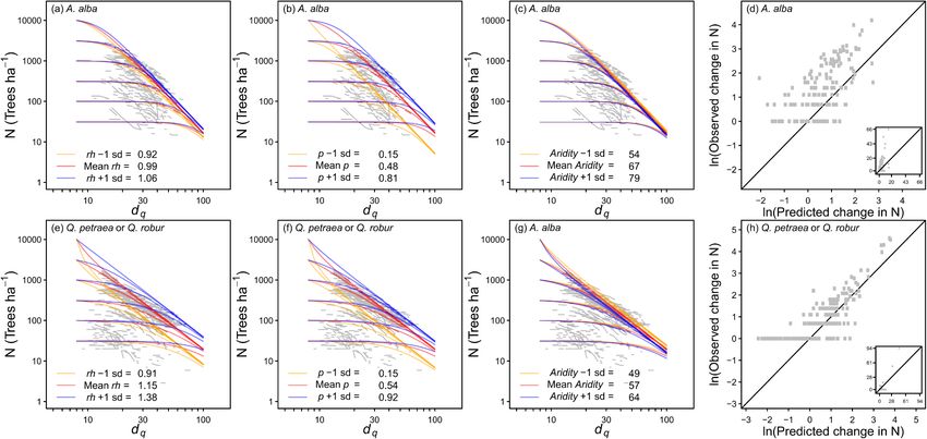
D.I. Forrester et al. Forest Ecology and Management 487 (2021) 118936
1. Introduction
dN
= − eβ 0 × Sβ1 × N β 2 , (6)
dS
Many decades after the development of indices of the effects of
density on self-thinning and of maximum size – density relationships in where N is tree density, S is the mean size of the trees, and β0, β1 and β2
even-aged monospecific forests (Reineke, 1933; Yoda et al., 1963) there are constants. This enables the simulation of the conditions that cause
remains debate about data selection and statistical methods for fitting tree density to decline, even before the stand reaches the theoretical
the relationship (Vanclay and Sands, 2009; Burkhart and Tomé, 2012; frontier. It also makes use of all data, not only data close to the theo
Trouvé et al., 2017). Moreover, self-thinning relationships for mixed- retical frontier, and therefore reduces potential subjectivity of data
species or uneven-aged forests have received much less attention than selection.
even-aged monocultures. Eq. (6) can be solved, with the separation of variables method, to
Self-thinning relationships are often described as a straight-line obtain N as a function S, from which the following self-thinning line can
relationship between logarithmically transformed tree density versus be derived (Supplementary material S1.2 of Trouvé et al., 2017):
mean tree size:
( ) ln(N) = intercept + slope × ln(S) (7)
ln(N) + 2ln dq = intercept (1)
where
( ) β0 ln(β2 − 1) − ln(β1 + 1)
ln(N) + 1.605ln dq = intercept (2) intercept = + , (8)
1 − β2 1 − β2
1 + β1
2
ln(N) + ln(v) = intercept (3) slope = . (9)
3 1 − β2
From the solution of Eq. (6), a self-thinning trajectory can be derived
3
ln(N) + ln(m) = intercept (4) that predicts tree density at the end of a period Nt2 as a function of the
4
density at the start of the period Nt1 and the mean tree size at the start St1
1 ( ) and end St2 of the period (Trouvé et al., 2017):
ln(N) + ln h = intercept, (5)
2 ( )1− 1β
1 − β2 ( β1 +1 )
(10)
2
Nt2 = Nt11− β2
+ eβ0 × × St1 − Sβt21 +1 .
where N is the tree density (i.e. number of trees per unit area), dq is the β1 + 1
quadratic mean tree-stem diameter, v is the mean tree-stem volume, m is The slopes and intercepts of Eqs. (2), (3) and (7) can differ between
the mean tree mass, and h is mean tree height. When these relationships species (Puettmann et al., 1993; Pretzsch and Biber, 2005; Pretzsch,
are fitted to data on the “frontier” (outer edge) of a data set, they provide 2006; Aguirre et al., 2018; Pretzsch and del Río, 2020), the shape of tree
a self-thinning line that is assumed to represent a barrier such that any size distributions (Sterba and Monserud, 1993; Gül et al., 2005), the
further increase in mean tree size is only possible if the density of trees environmental conditions (Zeide, 1987; DeBell et al., 1989; Hynynen,
declines along the self-thinning line. This theoretical frontier or barrier 1993; Bi, 2001; Yang and Titus, 2002; Morris, 2003; Weiskittel et al.,
has been given different names, including the maximum density (Rein 2009; Comeau et al., 2010; Aguirre et al., 2018), stand age (Ogawa,
eke, 1933; Eq. (2)), self-thinning line (Yoda et al., 1963; Eq. (3)), 2005; Zeide, 2005; Poage et al., 2007), and whether in mixed compared
maximum population density (Enquist et al., 1998; Eq. (4)) or natural with monospecific forests (Binkley, 1984; Puettmann et al., 1992;
basal area (Pienaar and Turnbull, 1973; Vanclay, 1994). Additional Woodall et al., 2005; Weiskittel et al., 2009; Ducey and Knapp, 2010;
variations have also been proposed (García, 2009; Eq. (5)), including the Reyes-Hernandez et al., 2013; Pretzsch et al., 2015). Accounting for
competition density rule (Sterba, 1987). these effects may be achieved more easily by using rates of change in N
These equations are useful simplifications of stand-level allometry, and S because they simply start from one point and go to the next, rather
and Eqs. (2) and (3) have been used in forest growth models to predict than being restricted to self-thinning frontiers (García, 2011).
density-dependent mortality (e.g. Landsberg and Waring, 1997; Bur Self-thinning equations calibrated for a specific combination of
khart and Tomé, 2012; Härkönen et al., 2019). A limitation is that species (e.g. Binkley, 1984; Puettmann et al., 1992; Pretzsch and For
contrary to the implications of Eqs. (1)–(5), self-thinning can begin rester, 2017) are limited to that species combination and often do not
before the stand actually reaches the self-thinning line, not “at” the line quantify the effect of species proportion, which may change between
(e.g. Drew and Flewelling, 1979), and many methods used for the cali stands and with stand age. Stand-level and cohort-level forest growth
bration of the relationships require a selection of data that are assumed simulation models require self-thinning equations that can predict
to be at the theoretical self-thinning frontier (Vanclay and Sands, 2009; changes in stand density for each cohort (species, size class, age class)
Burkhart and Tomé, 2012). Self-thinning relationships can also vary and any combination of species, size classes or age classes that it is
depending on the methods used to calibrate them, e.g. ordinary least competing with.
squares, non-linear least squares, reduced major axis, stochastic frontier The species or tree size cohort composition can be quantified as the
analysis, quantile regression, segmented regression, generalized linear proportion of the stand density (for example as tree density, or basal
models with different error distributions (e.g. Poisson, negative bino area) contributed by that species or size cohort (García, 2013). However,
mial) (Pretzsch and Biber, 2005; Zhang et al., 2005; Burkhart and Tomé, for a given tree size (diameter, height, etc.), different species have
2012; Possato et al., 2016; Trouvé et al., 2017), and they tend to be very different competitive abilities, so self-thinning patterns for a given
data demanding to calibrate (Vanclay and Sands, 2009). Moreover, species will probably differ depending on whether it is mixed with a
managed stands do not often lie close to posited self-thinning frontiers, strong competitor, or a weaker competitor. Based on an analysis of
somewhat limiting their practical significance (García, 2011). 140,000 plots across the world Kunstler et al. (2016) found that as stem-
To overcome these limitations, several studies have suggested wood density increased, there was a decrease in the growth response to
modelling changes in tree density relative to changes in tree size instead neighbourhood basal area from other species and the competitive effect
of the state variables (Eqs. (1)–(5)) (García, 2009; Vanclay and Sands, on other species increased. Although stem-wood density can vary for a
2009; García, 2011; Trouvé et al., 2017): given species (e.g. with growth rate, age, resource availability, climate
and silviculture (Beadle et al., 2011; Pretzsch et al., 2018; Rocha et al.,
2020)), it may still quantify some of the effects of species composition on
2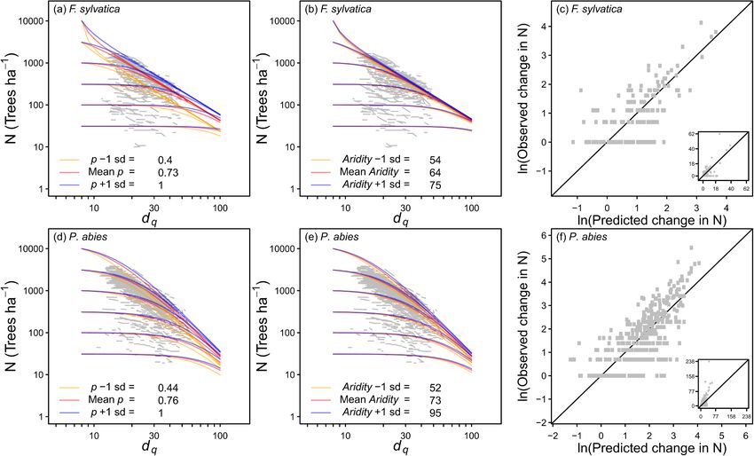
D.I. Forrester et al. Forest Ecology and Management 487 (2021) 118936
self-thinning. Species composition could be quantified as a species equations are to be applied, such as a wide range of stand basal areas,
proportion (p) in terms of the contribution the given species makes to the mean diameters, tree densities, species compositions, and vertical
stand basal area weighted by the species competitive ability as expressed structures, while not having any recruitment or applied thinning during
by wood basic density. Similarly, the mean stand wood basic density was the periods examined. Such data sets are not often available for many
used to quantify stand density indices in mixed forests of North America species or species mixtures (Woodall et al., 2005; Ducey and Knapp,
(Woodall et al., 2005; Ducey and Knapp, 2010). 2010). A possible solution to this problem is to develop all-species
Vertical stand structure may also need to be accounted for because equations, where data from many species are combined. This requires
the mortality rates for a given species or size cohort could depend on that species identity can be quantified using a variable that is correlated
canopy position (dominant, subdominant, etc). Vertical structure can be with inter-specific differences in self-thinning patterns.
quantified as the relative height (rh), which is the mean height of the Several studies have found that the basic density of the wood of a
object species (or cohort) divided by the mean height of all trees in the species is negatively correlated with maximum stand density indices and
stand. hence self-thinning patterns (Dean and Baldwin, 1996; Woodall et al.,
The use of species or size cohort proportions (p) and relative height 2005; Ducey and Knapp, 2010; Ducey et al., 2017; Andrews et al., 2018).
(rh) would extend Eq. (6) to The reasoning is that for a given diameter, species with higher wood
densities can support larger branches and leaf areas and therefore fewer
dN
= − eβ0 × Sβ1 × N β2 × rhβ3 × pβ4 . (11) trees per unit area are required to close the canopy; species with higher
dS
wood densities should have lower maximum stand density indices (Dean
Like Eq. (6), Eq. (11) can be solved to obtain N as a function of S (and and Baldwin, 1996). Shade tolerance has also been considered, however,
rh and p), and from this solution the intercept parameter for the self- it is less consistently correlated with maximum stand density indices
thinning line of Eq. (7) can be derived (the slope parameter is as (Lonsdale, 1990; Jack and Long, 1996; Woodall et al., 2005; Weiskittel
shown by Eq. (9)): et al., 2009; Charru et al., 2012; Ducey et al., 2017; Andrews et al.,
β0 ln(β2 − 1) − ln(β1 + 1) + β3 × ln(rh) + β4 × ln(p) 2018). Shade tolerance is also a complex variable that is unavailable for
intercept = + . many species, thereby reducing its practicality. While these traits have
1 − β2 1 − β2
been used to develop all-species stand density index equations, we are
(12)
not aware of any self-thinning equations that have been developed using
The self-thinning trajectory function becomes such traits.
( )1− 1β The first objective of this study was to examine how species pro
1− β2 1 − β2 ( β1 +1 β β β +1 β β ) 2
portion, relative height, site quality and climate affect self-thinning. It
Nt2 = Nt1 + eβ0 × × St1 × rht13 × pt14 − St21 × rht23 × pt24 .
β1 + 1 was hypothesized that the intercept of self-thinning lines will be greater
(13) when (1) the species proportion of the object species decreases
Self-thinning equations also need to be appropriate for stands with (assuming generally positive mixing effects on stand density), (2) a
different size or age distributions, such as from even-aged forests with species is more dominant, in terms of relative height, and (3) as climatic
unimodal-shaped distributions to single-tree selection forests with or edaphic conditions improve site quality. The second objective was to
reverse-J-shaped distributions. That is, except where there is no signif examine whether species traits could be used to develop all-species self-
icant relationship between tree size and mortality rate, the shape of the thinning equations by adding trait variables to Eqs. (11), (12) and (13).
size distribution will influence the stand mortality rate because the size
distribution defines how much of the stand density is composed of a 2. Material and methods
given tree size, and hence the proportion of the stand composed of tree
sizes susceptible to mortality (Forrester, 2019). That size distributions 2.1. Experimental sites
influence self-thinning patterns has been known for several decades
(Sterba and Monserud, 1993), and the effect can be at least partly Data were obtained from permanent sample plots and long-term
accounted for by applying Eq. (13) to several cohorts assumed to have silvicultural experiments in natural and planted forests in Australia,
roughly unimodal-shaped distributions, instead of treating the whole China and Switzerland. The Australian data (436 plots from 29 sites)
stand as a single cohort. Thus, the response of each cohort can differ were from Eucalyptus plantation experiments in temperate and Medi
depending on the exponents β3 and β4 (Eqs. (11) and (13)), and the terranean climatic regions, examining planting spacing, thinning, fer
response of the entire stand will be the sum of all the cohorts. tiliser application or species mixing (Table 1). The Chinese data were
Dividing a stand into cohorts has also been used to avoid the issue of from tree-species rich subtropical forests (88 Chinese national forest
Jensen’s inequality (Jensen, 1906) when calculating stand density inventory plots). The Swiss data were from temperate forests that were
indices based on Eq. (2), i.e. the mean of a function is not necessarily the either unmanaged, including 71 plots from 21 sites in the Swiss Forest
same as the function of the mean. For example, several studies have Reserve Research (FRR) network (Hobi et al., 2020), or experiments in
calculated stand density indices by summing the stand density index for managed forests, including 984 plots from 594 sites in the Experimental
each size class within a stand (Stage, 1968; Long and Daniel, 1990). Forest Management (EFM) network (Forrester et al., 2019). We only
However, this approach can potentially produce biased estimates by included data from plots where there were at least 5 trees of the object
overestimating the relative density of small size classes (Woodall et al., species, and it existed as a single cohort (determined by visual inspection
2003). Summation approaches have also been applied to mixed-species of size distributions). This still resulted in negative exponential shaped
forests (Woodall et al., 2005; Ducey and Knapp, 2010; Ducey et al., size distributions in the data set, but was done to avoid introducing
2017). potential subjectivity from dividing an object species into multiple
Eq. (11) may need to account for the effects of climatic and edaphic cohorts.
factors on self-thinning relationships. A potential site effect is consistent
with suggestions to use dominant height as the size variable (García, 2.2. Climate data
2009). However, Trouvé et al. (2017) suggested that mean diameter
would be appropriate because it is more closely related to crown width The effect of climate on self-thinning was quantified using an aridity
and space occupancy. index (de Martonne, 1926) that was calculated for each site as (mean
The fitting of self-thinning equations (e.g. Eqs. (1)–(5)) requires annual precipitation in mm) ÷ (mean annual temperature in ◦ C + 10).
relatively large data sets that include most situations where the The mean temperatures and precipitation used to calculate the aridity
index were obtained: (i) for the Australian sites from interpolated
3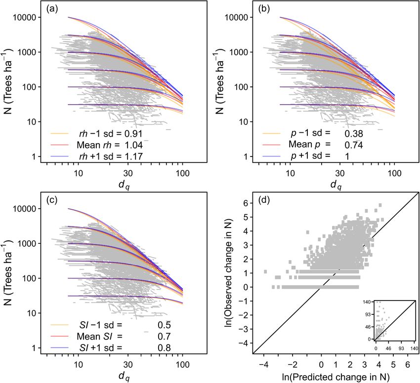
D.I. Forrester et al. Forest Ecology and Management 487 (2021) 118936
national climate surfaces ANUCLIM MTHCLM (Xu and Hutchinson, was quantified using relationships between dominant height and age. In
2011), (ii) for the Swiss sites by interpolation (after Thornton et al. monocultures, the dominant height was the mean height of the largest-
(1997)) from data collected by the Federal Office of Meteorology and d 100 trees ha− 1. In mixtures, to avoid underestimating the site index,
Climatology MeteoSwiss. For the Chinese data, monthly precipitation the dominant height was calculated from fewer trees: [100 × species
and temperature were calculated by spatial interpolation of climate data proportion in terms of basal area] trees ha− 1. The relationship between
collected at 369 meteorological stations in Hunan Province (Zhao et al., dominant height and age for a given species was estimated by fitting all
2013). the data for the species to a von Bertalanffy equation (Pienaar and
Turnbull, 1973)
2.3. Tree measurements Hd = aH [1 − exp( − bH A)]cH , (15)
In the Australian plots, tree diameter at 1.3 m height (d) was where Hd is the dominant height (m), A is age (years) and aH, bH and cH
measured for all trees when they were at least 1.3 m tall, and tree height are parameters. Eq. (15) was fit as a non-linear model using the nlxb
(h) was measured on either all trees or a sample spanning their size function of the nlmrt package (Nash, 2016) in R (R Core Team, 2019).
range. For some sites, crown diameters were also measured for a sample The SI was then calculated from
of trees. In the Chinese plots, d was measured on all trees with d ≥ 5 cm,
[1 − exp( − bH Ar )]cH
but no heights were measured. In the Swiss EFM plots and FRR plots, SI = Hd , (16)
d was measured on all trees with d ≥ 8 cm or d ≥ 4 cm, respectively, and [1 − exp( − bH A)]cH
tree heights and four crown radii were measured for a sample of trees
where Ar is the reference age for SI: 10 years for the Australian plots,
(the 100 largest-diameter trees ha− 1 and 20% of the rest). Unmeasured
which were relatively faster growing, and 100 years for Swiss plots,
tree heights in the Australian and Swiss plots were estimated using plot-,
which were slower growing. SI could not be calculated for the Chinese
year- and species-specific regressions after Forrester et al. (2019). The
plots because height data were not available.
measurement intervals for the Australian, Chinese and Swiss plots varied
between about one and twelve years, depending on silvicultural treat
2.5. All-species equations
ments and growth rates. In the data we only included growth periods
without any recruitment.
Three species traits were used to examine whether they could be used
to develop all-species self-thinning equations: (i) wood basic density (ρ),
2.4. Calculations (ii) specific leaf area (SLA, m2 kg− 1), and (iii) the relationship between
tree crown diameter (cd, m) and stem diameter (d). These values were
For each species in each plot, quadratic mean d (dq ), tree density (N, obtained from literature review (Table A1). The cd–d trait was deter
trees ha− 1), species proportion (p), and relative height (rh) were mined as the two parameters aC and bC in the equation
calculated for alive trees at each measurement age. Changes in N (ΔN)
cd = aC dbC . (17)
and dq (Δdq ) between successive pairs of measurements were annualised
by dividing by the length of the observation period. Because of the These parameters were used because for a given d, species with
highly diverse species composition of the Chinese plots, N for each longer branches may require fewer trees per unit area to close the can
species was too small for species-level analyses and therefore the species opy, and thus may manifest inter-specific differences in self-thinning.
were not differentiated and p and rh were not calculated. For all other The cd–d parameters were previously calculated from crown diameter
mixed-species plots, the N of a given species was divided by its pro measurements in the EFM and FRR plots for the Swiss species (Forrester
portional contribution to stand basal area to provide a monoculture et al., 2021), and for E. nitens by Forrester et al. (2012a) (Table A1).
equivalent. This was required because the self-thinning equations are for E. globulus cd–d parameters were calculated using data from the exper
individual species or cohorts, so regardless of whether they are growing iment described in Forrester et al. (2011), which is also included in this
in a mixture or monocultures, the N of an object species needs to study.
represent that N that would exist in a monoculture that has the same To determine any inter-specific differences in self-thinning, the slope
total stand basal area as the mixture. The species proportion was and intercept as in Eqs. (1) and (2) were calculated from the parameters
quantified in terms of the contribution the object species made to stand of the species-specific equations (e.g. Eqs. (13)) using Eqs. (9) and (12).
basal area (G, m2 ha− 1) weighted by the wood basic density (ρ; oven dry The slope and intercepts were then regressed against the traits.
mass per fresh volume; g cm− 3): The all-species equations were based on Eq. (11), but each explan
atory variable was replaced with an interaction between the given
G i × ρi
pi = ∑n . (14) variable and an individual trait or trait parameter. In order to include
i=1 Gi × ρi each species in the all-species equation, SI and aridity index were con
This weighting was to represent inter-specific differences in growth strained to a maximum of 1. That is, the index for a given species was
responses to neighbourhood basal area (competitive ability) for a tree of divided by the maximum value for that species. This normalisation was
a given d, which has been found to be correlated with ρ (Kunstler et al., required because some species can, on average, occur on sites with
2016). For a given proportional contribution to basal area, p will be higher SI or aridity indices than others and thus confound species effects
lower when a species is mixed with a high-wood-density species than with the SI or aridity effects.
when it is mixed with a low-wood-density species. A p of 1 indicates that
the species is in a monoculture, or that all species have the same wood 2.6. Model fitting
density. The ρ for each species was obtained from the literature
(Tables A1 and A2). The self-thinning lines (Eqs. (9) and (12)) and self-thinning trajectory
Because the aridity index will only partly account for all site effects functions (Eq. (13)) were calibrated by fitting the rate of change equa
(climatic and edaphic), a site (quality) index was also calculated. While tion (Eq. (11)) as a generalized linear model (GLM) with random effects.
this will be influenced by the climatic factors that influence the aridity Eq. (11) was transformed into
index, the aridity index and site index were not correlated for any of the ( ) ( )
species in this study and both indices were used to make comparisons log(ΔN) = β0 + β1 log dq + β2 log(N) + β3 log(rh) + β4 log(p) + log Δdq
with previous studies where these indices have been used to examine
(18)
self-thinning relationships. Site index (SI, m) for each species at each site
4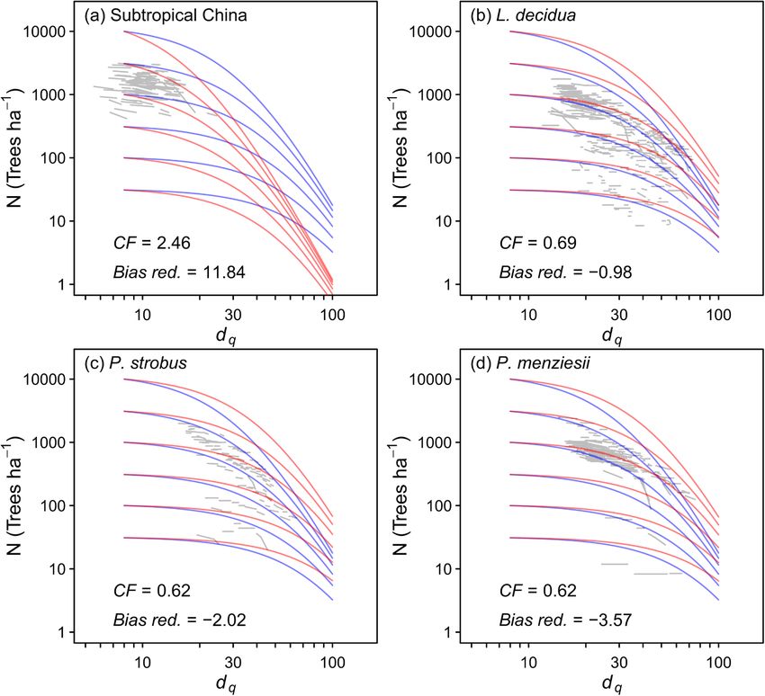
D.I. Forrester et al. Forest Ecology and Management 487 (2021) 118936
by approximating the differentials (dN,dS = ddq ) with differences ( − ΔN, where the notation is as above.
ΔS = Δdq ) and by taking the logarithm on both sides. By considering the When using zero-inflated and hurdle distributions, the probability
mortality count ΔNijk of observation period k on plot j on site i as a πijk generating extra zeros was modelled with a GLM involving Bernoulli
( )
( )
random variable with a discrete probability distribution, Eq. (18) could distribution, logit link function and log dq,ijk or log Nijk or both as the
( )
be described as a GLM with a logarithmic link function and log Δdq as explanatory variables.
an offset term: The models were fitted using the glmmTMB function in the R package
glmmTMB (Brooks et al., 2017). An example R script to fit these models is
where μijk = E(ΔNijk ) is the mean of the distribution of ΔNijk , assumed to provided as supplementary material.
To evaluate the goodness-of-fit for each model, we calculated the
depend on the observed values of dq,ijk , Nijk , rhijk , and pijk in the beginning mean of prediction errors
of the period k and of Δdq,ijk during the period k, and bi and bij are ( )
∑
random effects for the site and for the plot within each site, respectively, yk − ̂
yk
assumed to be independent and normally distributed with means 0 and Bias = (22)
separate constant variances. The random effects account for the n
dependence between the repeated measurements on a plot, and between the root mean square error
multiple plots at the same site. √̅̅̅̅̅̅̅̅̅̅̅̅̅̅̅̅̅̅̅̅̅̅̅̅̅̅
Several models following Eq. (19) but with different probability ∑
y k )2
(yk − ̂
distributions for ΔNijk were compared. First, a model with Poisson dis RMSE = (23)
n
tribution (Poisson) was fitted (cf. Trouvé et al., 2017). The problem with
the Poisson distribution is that it involves only one parameter (mean μijk ) and the coefficient of determination
and assumes the variance to be equal to the mean, whereas in practice ∑
count data are more dispersed. To deal with the problem of over (yk − ̂y k )2
R2 = 1 − ∑ (24)
dispersion, a model with a negative binomial distribution (NB) was also (yk − y)2
fitted (cf. Affleck, 2006; Trouvé et al., 2017). This distribution involves
an additional dispersion parameter, which can depend on the mean where yk and ̂
y k are the observed and the fitted values of mortality count
linearly or quadratically; in this study, the parameterisation with ΔNk for period k. All analyses were performed using R software (R Core
( )
quadratic dependence was used (Var ΔNijk = μijk + μijk 2 /θ, where θ is Team, 2019). The best models for each species were generally consid
ered those with the lowest AIC and BIC, but visual inspection of pre
the dispersion parameter).
dicted and observed ΔN, and the other statistical information in Table 2
In the data, the number of zero mortality counts was likely to be
were also used.
larger than what would be predicted by a Poisson or negative binomial
model. To deal with the problem of zero-inflation, models with zero-
3. Results
inflated, or hurdle, Poisson (ziP, hP) and negative binomial (zNB,
hNB) distributions were fitted. These distributions involve a separate
Self-thinning trajectories were fit for species with at least 100 pairs of
process that generates extra zeros with probability πijk .
successive measurements (Table 2). Fits using smaller sample sizes were
A zero-inflated distribution (Lambert, 1992; Greene, 1994) assumes
less reliable, based on the statistics used to judge the quality of fit and a
two types of observation periods: those where mortality can never occur
visual inspection of the predicted self-thinning trajectories.
(ΔN is always zero; source of extra zeros), and those where mortality can
While there were often differences in parameter estimates depending
occur but does not always (normal mortality process). Zero mortality
on the models used (Table 2), there were generally only minor differ
( ) ( )
( ) ( ) ( ) ( )
log μijk = β0 + β1 log dq,ijk + β2 log Nijk + β3 log rhijk + β4 log pijk + log Δdq,ijk + bi + bij (19)
counts can thus come from both types of periods. The zero-inflated ences in the predicted self-thinning trajectories (results not shown), and
probability distribution function is no fitting type was consistently better or worse than the others. The sign
{ ( ) ( ) of the parameters, indicating the direction of the relationship, was the
{ } πijk( + 1 − )πijk( f 0; Θ
Pr ΔNijk = m = ) ijk , m = 0 (20) same for a given variable and species.
1 − πijk f m; Θijk , m > 0,
Relative height (rh) was significant for A. alba, Q. petraea and
Q. robur, such that mortality declined as the relative height (i.e. domi
where f is the probability distribution function of Poisson distribution
nance) increased (Fig. 1). This could not be tested for the Eucalyptus
with parameter Θijk = μijk or negative binomial distribution with pa
species or P. sylvestris because there was not enough range in rh for these
rameters Θijk = (μijk , θ).
shade intolerant species. Relative height had no significant effect on the
A hurdle distribution (Cragg, 1971; Mullahy, 1986) assumes that the self-thinning of F. sylvatica or P. abies.
observation periods are either where mortality can never occur, or Species proportion (p) was significant for 4 of the 5 species where it
where mortality always occurs (at least one dead tree is observed). Here, could be tested (was not significant for P. sylvestris) (Figs. 1 and 2). In all
zero mortality counts can thus come only from periods of the first type. cases the mortality rates declined as the proportions of the object species
The hurdle probability distribution function is increased. The aridity index was significant for all species except Euca
⎧
π ijk , m = 0 lyptus (Figs. 1 and 2; Table 2). The mortality rates declined with
⎪
{ } ⎨ ( ) increasing moisture for P. abies and F. sylvatica, but increased for A. alba,
Pr ΔNijk = m = ( ) f m; Θijk (21)
⎪
⎩ 1 − π ijk ( ), m > 0, P. sylvestris and Quercus. Site index (SI) was significant for P. sylvestris
1 − f m; Θijk and E. globulus, and in both cases the rates of self-thinning decreased as
5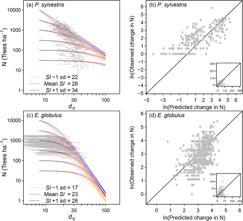
D.I. Forrester et al. Forest Ecology and Management 487 (2021) 118936
Table 1
Summaries of plot and site characteristics for the 11 object species, as well as the species-diverse subtropical forest in China. dq is quadratic mean of tree diameters at
1.3 m height, p is the proportion of stand basal area contributed by the object species, and rh is the relative height of the object species (mean height of trees of object
species divided by mean height of all trees in the plot).
Abies Eucalyptus Eucalyptus Fagus Fraxinus Larix Picea Pinus Pinus Pseudotsuga Quercus Subtropical
alba globulus nitens sylvatica excelsior decidua abies strobus sylvestris menziesii petraea or China
Q. robur
Number of plots 104 326 110 217 61 135 393 26 191 55 165 88
First/last 1888/ 1993/2019 1998/ 1889/ 1889/ 1889/ 1888/ 1891/ 1889/ 1906/2018 1889/ 2009/2014
measurement 2018 2015 2019 2017 2019 2019 1995 2019 2019
Mean plot size 0.38 0.07 0.09 0.33 0.44 0.38 0.29 0.29 0.22 0.2 (0.02/ 0.39 0.07 (0.07/
(min/max) ha (0.04/ (0.02/ (0.03/ (0.01/ (0.06/ (0.02/ (0.02/ (0.06/ (0.01/ 0.84) (0.02/ 0.07)
1.22) 0.14) 0.13) 1.22) 1.65) 1.65) 1.22) 0.53) 1.54) 3.06)
Mean basal area 51.7 19.4 (3.4/ 23 (4.7/ 35.2 39.2 36.9 49.4 44.9 37.5 (4/ 43.3 (20.8/ 28.6 12.4 (1.9/
(G) (min/max) (9.6/ 81.3) 56.6) (7.1/73) (19/70) (7.3/73) (8.6/ (26.1/ 140.2) 81.5) (4.3/ 29.7)
m2 ha− 1 84.1) 107.2) 76) 87.6)
Mean dq (min/ 29.9 20.9 (6.2/ 26.6 25.2 25.9 33.2 25.5 32 26.3 29.9 (14.4/ 28.5 (9/ 10.2 (5.5/
max) cm (10.8/ 46.9) (13.1/ (11.5/ (11.4/ (11.8/ (10.6/ (15.5/ (11.8/ 66.9) 75.4) 22)
62.7) 47.5) 52.1) 55.7) 70.8) 57.3) 61.7) 68.6)
Mean tree 446 582 (131/ 473 (100/ 485 (10/ 121 (8/ 355 (8/ 990 543 573 (10/ 630 (8/ 210 (3/ 1480 (507/
density (min/ (15/ 1718) 1735) 1664) 946) 1769) (19/ (29/ 4814) 2500) 1700) 3119)
max) ha− 1 2779) 3840) 1988)
Mean p (min/ 0.48 0.94 1 0.73 0.16 0.66 0.76 0.74 0.61 0.92 (0.01/ 0.51 *
max) (0.01/ (0.11/1) (0.01/1) (0.02/1) (0.02/1) (0.01/ (0.02/ (0.02/1) 1) (0.01/1)
1) 1) 1)
Mean rh (min/ 0.99 1.02 1 0.98 1.06 1.13 1.01 1.11 1.11 1.03 (0.98/ 1.15 *
max) (0.51/ (0.93/ (0.52/ (0.86/ (0.94/ (0.56/ (1/ (0.76/ 2.13) (0.69/
1.52) 1.47) 1.38) 1.41) 1.73) 1.95) 1.51) 1.53) 2.7)
Mean daily 23 26.6 24.7 23.3 23.1 22.2 22.4 23.8 23.2 24.1 (20.2/ 24 (20.2/ 33.5 (32.8/
maximum (17.4/ (23.9/ (21.1/ (17.4/ (21.1/ (16.2/ (15.3/ (19/ (14.9/ 26.2) 28.4) 34.5)
temperature in 26.6) 30.2) 29.7) 26.4) 25.3) 27.4) 26.6) 26.6) 28.4)
warmest
month (min/
max) ◦ C**
Mean daily − 3.7 4.8 (2.1/ 3.4 (2.1/ − 3.2 − 2.6 − 4.7 − 3.9 − 3.4 − 3.9 − 2.5 (− 7/ − 2.6 2.2 (1.5/
minimum (− 7/ 8.2) 4.4) (− 7/ (− 5/ (− 12.8/ (− 11/ (− 7.4/ (− 10.6/ − 1.3) (− 7/ 2.8)
temperature in − 0.9) − 0.3) − 1.2) 0.9) 0.1) − 0.5) − 0.5) − 0.9)
coldest month
(min/max)
◦
C**
Mean 1202 829 (457/ 1163 1179 1221 1147 1273 1202 1104 1204 (929/ 1074 1403
precipitation (898/ 1172) (794/ (853/ (927/ (744/ (823/ (899/ (631/ 1993) (646/ (1286/
(min/max) 1860) 1324) 1860) 1711) 2025) 2049) 1979) 2025) 1749) 1620)
mm yr− 1
Aridity index 67 34 (18/47) 52 (32/62) 64 (45/ 66 (47/ 67 (39/ 73 65 (46/ 62 (31/ 63 (48/121) 57 (31/ 50 (46/58)
(min/max) (46/ 108) 100) 140) (45/ 105) 107) 100)
108) 155)
*
not calculated due to the high species diversity that resulted in lower sample sizes for any given object species.
**
January and July were considered the warmest and the coldest month in the southern hemisphere, respectively, and the coldest and the warmest month in the
northern hemisphere, respectively.
Table 2
Parameter estimates and fit statistics for self-thinning models based on Eqs. (11) and (13) (for model types listed in the first column, see Methods). OD = overdispersion
parameter for models with negative binomial distributions; X = variance for the random effects of site and plot, if included in model; AIC = Akaike’s information
criterion; BIC = Bayesian information criterion; RMSE = square root of the mean square error (units = ΔN); Bias, calculated mean of the differences between observed
ΔN and predicted ΔN (units = ΔN)). Note that for individual species equations the site index and aridity index were not standardised, as opposed to the all-species
equation.
Species / β0 β1 (dq ) β2 (N) β3 (rh) β4 (p) β5 β6 (SI) OD X= X= AIC BIC R2 RMSE Bias
Model (Aridity) site/ site
plot
Picea abies
NB − 19.42 2.3 2.17 − 1.03 0.80 0.29 0.041 5913 5949 0.47 11.43 1.16
(3.05) (0.45) (0.24) (0.26)
*Poisson − 20.91 3.7 2.71 − 1.43 − 1.56 1.35 0.000 3610 3640 0.91 5.25 0.02
(2.62) (0.36) (0.19) (0.24) (0.25)
ziNB − 11.02 0.87 1.65 − 0.47 1.19 5802 5847 0.29 13.18 0.64
(2.12) (0.31) (0.17) (0.18)
ziP − 9.90 1.57 2.07 − 1.01 − 0.51 − 1.1 3896 3935 0.42 13.56 0.15
(1.06) (0.13) (0.07) (0.09) (0.09) (0.16)
hNB − 12.21 1.43 1.85 − 0.75 − 0.59 1.56 0.12 0.015 5761 5817 0.43 11.99 1.16
(2.81) (0.39) (0.2) (0.24) (0.28)
hP − 12.02 1.53 1.82 − 0.71 − 0.49 0.36 0.019 3069 3112 0.82 7.47 0.24
(2.41) (0.36) (0.19) (0.23) (0.24)
(continued on next page)
6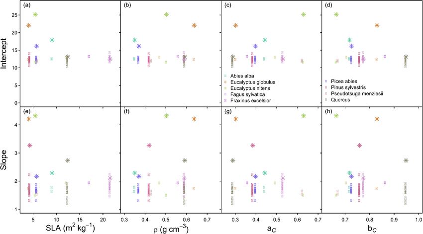
D.I. Forrester et al. Forest Ecology and Management 487 (2021) 118936
Table 2 (continued )
Species / β0 β1 (dq ) β2 (N) β3 (rh) β4 (p) β5 β6 (SI) OD X= X= AIC BIC R2 RMSE Bias
Model (Aridity) site/ site
plot
Abies alba
NB − 18.18 2.46 1.85 − 5.76 − 0.91 2.19 0.13 0.554 1509 1541 0.72 3.82 0.34
(5.98) (0.91) (0.45) (1.32) (0.46)
*Poisson − 31.07 3.71 2.55 − 5.41 − 1.58 0.96 0.15 0.926 924 954 0.89 2.84 0.01
(6.71) (0.96) (0.46) (1.14) (0.48) (0.43)
hP − 12.9 1.43 1.61 − 0.93 0.31 0.153 1587 1618 0.77 3.47 0.52
(4.56) (0.69) (0.34) (0.36)
Pinus sylvestris
Poisson − 30.17 3.04 3.38 − 1.72 3 (0.36) − 3.48 0.34 3857 3889 0.9 7.32 0.01
(3.18) (0.44) (0.21) (0.24) (0.47)
ziP − 21.31 0.59 1.79 3.41 − 0.97 0.50 1.390 2114 2171 0.8 10.57 0.31
(3.15) (0.37) (0.16) (0.46) (0.47)
*hP − 23.36 0.82 1.88 3.63 − 1.08 0.52 1.787 2117 2174 0.79 10.66 0.08
(3.18) (0.4) (0.17) (0.47) (0.5)
Fagus sylvatica
NB − 30.4 4.37 2.7 − 2.28 1.17 0.59 0.765 1721 1753 0.63 2.49 0.26
(5.4) (0.83) (0.44) (0.44)
Poisson − 33.26 4.48 3.07 − 2.51 0.91 0.900 1819 1846 0.87 1.48 0.02
(4) (0.6) (0.33) (0.35)
ziNB − 18.54 2.18 2.1 − 1.16 5.38 0.24 0.577 1663 1722 0.72 2.17 0.17
(5.85) (0.87) (0.49) (0.47)
*ziP − 19.51 2.37 2.81 − 1.78 − 0.82 1050 1088 0.6 3.42 0.12
(2.17) (0.37) (0.18) (0.2) (0.33)
hNB − 19.47 2.4 2.17 − 1.4 4.67 0.13 0.396 1723 1782 0.63 2.51 0.39
(4.84) (0.74) (0.4) (0.41)
hP − 19.24 2.31 2.18 − 1.39 0.26 0.372 1739 1793 0.77 1.98 0.28
(4.28) (0.64) (0.36) (0.37)
Quercus petraea or Q. robur
NB − 19.29 2.28 2.31 − 4.24 − 1.29 1.22 0.03 0.365 1315 1349 0.58 5.2 0.39
(3.58) (0.6) (0.29) (0.85) (0.27)
Poisson − 26.34 2.97 3.08 − 3.79 − 1.91 0.56 0.343 1498 1528 0.91 2.44 0.01
(2.77) (0.48) (0.22) (0.76) (0.21)
*ziNB − 23.37 1.6 2.15 − 4.26 − 0.97 1.89 22.5 0.213 1088 1150 0.59 5.61 0.38
(3.51) (0.43) (0.19) (0.78) (0.18) (0.71)
ziP − 25.73 1.88 2.35 − 4.23 − 1.05 1.99 0.204 1120 1177 0.68 4.96 0.34
(3.12) (0.39) (0.17) (0.75) (0.15) (0.64)
hNB − 28.42 1.72 2.37 − 5.14 − 0.84 2.76 5.48 0.055 1140 1201 0.75 4.39 0.30
(4.42) (0.53) (0.22) (1.38) (0.17) (0.95)
hP − 32.19 0.46 1.91 − 4.4 5.4 (0.61) 1277 1318 0.2 7.85 − 0.08
(2.77) (0.33) (0.11) (1.01)
Eucalyptus globulus
NB − 21.37 2.98 3.35 − 2.05 0.25 0.41 0.611 4570 4604 0.19 16.48 − 0.01
(4.26) (0.67) (0.27) (0.83)
Poisson − 19.42 5.29 2.29 − 3.11 3.87 1.341 8742 8771 0.79 8.53 0.0024
(1.49) (0.2) (0.11) (0.33)
*ziNB − 9.76 1.95 1.62 − 1.05 3.36 0.06 0.188 4183 4232 0.42 14.04 0.72
(1.86) (0.43) (0.15) (0.41)
ziP − 11.86 3.5 1.82 − 2.28 0.22 0.309 4926 4969 0.56 12.23 0.84
(1.27) (0.21) (0.09) (0.29)
hNB − 9.52 1.93 1.6 − 1.06 3.38 0.06 0.183 4186 4235 0.42 14.09 0.74
(1.8) (0.42) (0.14) (0.4)
hP − 11.69 3.46 1.8 − 2.26 0.22 0.304 4929 4973 0.56 12.27 0.85
(1.26) (0.21) (0.09) (0.28)
Eucalyptus nitens
NB − 3.26 1.03 2.2 − 2.89 0.37 0.00 0.024 2149 2176 0.45 20 0.1838
(2.52) (0.77) (0.23) (0.79)
Poisson − 7.15 2.98 2.57 − 4.04 0.094 6218 6237 0.51 18.93 0.0001
(2.3) (0.14) (0.05) (0.6)
*ziNB − 3.53 1.73 1.6 − 2.83 3.16 0.333 1940 1982 0.46 19.94 0.3797
(3.13) (0.45) (0.13) (0.79)
ziP − 13.93 3.51 2.41 − 2.93 0.342 0.785 2305 2351 0.65 15.99 1.0093
(2.19) (0.21) (0.17) (0.44)
hNB − 3.57 1.74 1.6 − 2.82 3.21 0.331 1942 1984 0.46 19.96 0.4277
(3.11) (0.45) (0.13) (0.78)
hP − 13.67 3.49 2.38 − 2.92 0.33 0.765 2307 2353 0.65 16.04 1.0136
(2.13) (0.21) (0.16) (0)
All species
*NB − 17.38 1.86 2.05 − 2.18 − 0.92 − 0.54 0.48 0.24 0.481 21,468 21,527 0.52 11.34 1.04
(1.17) (0.19) (0.09) (0.39) (0.11) (0.2)
Poisson 1.78 0.872 26,984 27,040 0.84 7.17 0.00
(continued on next page)
7
D.I. Forrester et al. Forest Ecology and Management 487 (2021) 118936
Table 2 (continued )
Species / β0 β1 (dq ) β2 (N) β3 (rh) β4 (p) β5 β6 (SI) OD X= X= AIC BIC R2 RMSE Bias
Model (Aridity) site/ site
plot
− 33.39 4.41 3.29 − 2.77 − 2.08 0.33 − 0.38
(0.73) (0.11) (0.06) (0.2) (0.07) (0.13) (0.16)
ziNB − 5.67 0.32 1.08 − 2.01 − 0.63 2.38 0.12 0.306 20,291 20,388 0.52 11.36 0.80
(0.57) (0.11) (0.04) (0.33) (0.15)
ziP − 9.92 1.11 1.33 − 2.5 − 0.57 0.33 0.393 23,768 23,859 0.68 9.27 0.53
(0.44) (0.07) (0.03) (0.23) (0.11)
hNB − 6.53 0.38 1.19 − 1.75 − 0.65 2.25 0.10 0.262 20,274 20,371 0.53 11.28 0.92
(0.61) (0.12) (0.05) (0.36) (0.15)
hP − 11.23 1.28 1.46 − 2.33 − 0.59 0.32 0.336 23,744 23,835 0.7 8.92 0.57
(0.49) (0.08) (0.04) (0.25) (0.11)
All species (with only Size and N)
Poisson − 13.27 1.42 1.64 1.40 0.861 37,294 37,327 0.79 7.08 0.01
(0.41) (0.07) (0.03)
ziP − 6.08 0.27 1.21 0.34 0.434 31,263 31,316 0.47 11.33 0.36
(0.23) (0.04) (0.02)
*hP − 8.48 0.82 1.31 0.33 0.349 25,808 25,874 0.7 8.53 0.50
(0.41) (0.07) (0.03)
*
The best models for each species; selected based on the statistical information and visual inspection of graphs, and which were also used to produce Figs. 1, 2, 3, 5
and 7.
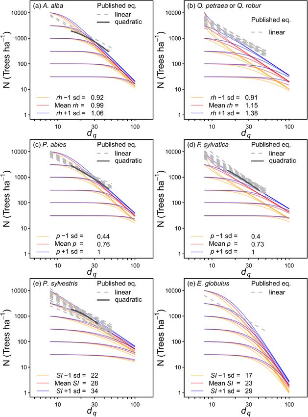
Fig. 1. Predicted self-thinning trajectories in comparison with observed data (grey lines), and the effects of relative height (rh) (a,e), species proportions (p) (b,f) and
the aridity index (c,g), and comparisons of observed and predicted changes in N (d,h) for A. alba, Q. petraea and Q. robur. Insets for (d) and (h) show non-transformed
data. The equations used to predict N are shown in Table 2. The sd is 1 standard deviation of the indicated variables.
site index increased (Fig. 3; Table 2). was applied as shown by Eq. (25) for the subtropical Chinese plots,
None of the species traits or trait parameters examined were related L. decidua, P. strobus, and P. menziesii (Fig. 6; Table 2). Since the Chinese
to the species-specific slopes or intercepts (calculated using Eqs. (9) and data did not contain the stand structural variables (rh and p), the all-
(12)) (Fig. 4). Therefore, the all-species models that included the traits species equation used also did not contain these variables, and is pre
are not presented. Instead all-species models were fit to all data without sented in Table 2. For the three conifers, the CF was negative indicating
differentiating between species (Fig. 5; Table 2). To apply this to species that before applying the CF, the all-species model overestimated rates of
for which there were not enough data, a species-specific correction self-thinning, whereas for the Chinese data, the all-species model
factor (CF) was calculated as the ratio of mean dN of measured data underestimated rates of self-thinning.
divided by the mean dN of the predicted data for the given species. This
Nt2 = Nt1 − CF × (Nt1 − [right side of Equation 10 or 13] ) (25)
8
D.I. Forrester et al.                                                                                                     Forest Ecology and Management 487 (2021) 118936

Fig. 2. Predicted self-thinning trajectories in comparison with observed data (grey lines), and the effects of species proportions (p) (a,d) and the aridity index (b,e),
and comparisons of observed and predicted changes in N (c,f) for F. sylvatica and P. abies. Insets for (c) and (f) show non-transformed data. The equations used to
predict N are shown in Table 2. The sd is 1 standard deviation of the indicated variables.

Fig. 3. Predicted self-thinning trajectories in comparison with observed data (grey lines), and the effects of site index (SI) (a,c), and comparisons of observed and
predicted changes in N (b,d) for P. sylvestris and E. globulus. Insets for (b) and (d) show non-transformed data. The equations used to predict N are presented in
Table 2. The sd is 1 standard deviation of the indicated variables.

                                                                                    9
D.I. Forrester et al. Forest Ecology and Management 487 (2021) 118936
Fig. 4. Scatter plots indicating the lack of relationships between species traits: specific leaf area (SLA), wood basic density (ρ), and cd–d parameters (aC and bC from
Eq. (17)) and the intercept and slope (e.g. of Eqs. (1) or (2)) that were calculated using Eqs. (9) and (12). The round symbols indicate published values (Table A1).
The star symbols were the fitted slope and intercept from the present study, which were calculated using rh = 1, p = 1, aridity index = 56 (mean for data set) and SI =
30 (mean for data set).
Fig. 5. Predicted changes in stand density (N ha− 1) in relation to quadratic mean diameter (dq) for all species combined, showing the observed data (grey lines) and
the effects of relative height (rh) (a), species proportion (p) (b) and site index (SI) (c), and comparisons of observed and predicted changes in N (d). Inset for (d) shows
non-transformed data. The equation used is described in Table 2. The sd is 1 standard deviation.
10D.I. Forrester et al. Forest Ecology and Management 487 (2021) 118936
Fig. 6. The all-species model applied to specific
species or the Chinese data after applying a species-
specific correction factor (CF). The blue lines are
the uncorrected all-species model, while the red lines
are the corrected model, the grey lines show the raw
data for the object species. The parameters for the
all-species model (containing only dq and N) are
shown in Table 2. The bias reduction (bias red.) is the
mean of the differences between observed dN and
predicted dN, and was reduced to 0 for all species
after applying the CF. (For interpretation of the ref
erences to colour in this figure legend, the reader is
referred to the web version of this article.)
study show that averaged across many species combinations, mixing
4. Discussion generally reduced potential maximum stand densities for a given spe
cies. The use of p assumes that the effects of species interactions on self-
Using rates of change to model self-thinning provided similar results thinning are correlated with the species proportion in terms of basal area
to previous studies that used state variables (Eqs. (1) and (2)) and weighted by the wood basic density of each species. If necessary, more
focused on data close to the self-thinning frontier (Fig. 7). However, the precise self-thinning equations could be developed by using data from a
slopes and intercepts in this study were often greater than those reported specific species mixture.
in the literature (Fig. 8). There is no reason that the equations in this
study are less accurate than those from the literature because they were
4.2. Effects of relative height and uneven-aged stands
based on large data sets, including many plots that had never been
thinned (e.g. E. globulus and E. nitens plots) or only lightly thinned, nor
Mortality rates declined as rh increased for each species where rh was
do the statistics suggest a low quality of fit. Instead the greater intercepts
significant (A. alba, Q. robur and Q. petraea). The higher mortality rates
and slopes in this study may have resulted from the less restrictive
with lower relative heights is consistent with findings of higher survival
equation form and data selection. Similarly, the non-linear self-thinning
rates with increasing light availability (Osunkjoy et al., 1992; Inman-
frontiers calculated by Charru et al. (2012) appear to be more consistent
Narahari et al., 2016). Relative height is rarely considered in mortality
with those in this study than in the studies that fit linear relationships,
studies, but these results indicate that the dominance of a species or
and several studies have suggested that self-thinning frontiers are not
cohort can be as influential as the effects of species proportions and
linear (Zeide, 1987; Cao et al., 2000). The greatest discrepancy was for
larger, as well as more consistent, than climatic effects such as those
large tree sizes, such that the linear relationships often predict that
quantified using the aridity index. The effect of rh on P. sylvestris or the
stands with dq = 100 cm will have at least 100 trees ha− 1, whereas the
Eucalyptus species could not be examined due to the small range in rh in
equations in this study predict lower stand densities.
the data set for these species. The small ranges resulted because these
species were often in monocultures or only occurred in the upper
4.1. Species mixing canopy.
By accounting for the effects of species or size cohort composition (p)
All stand structural and site variables influenced self-thinning re and the vertical position of each species or size cohort (rh), the equations
lationships. Self-thinning trajectories shifted upwards with increasing can be used for different cohorts within uneven-aged forests. Similarly,
species proportion p, indicating that monospecific stands supported the influence of size distributions on the self-thinning of a whole stand
higher densities than mixed-species stands. This was consistent, occur can be accounted for by calculating, and then summing, the changes in
ring for each species where p effects were significant; A. alba, F. sylvatica, the tree density of several cohorts. This could account for the effects of
P. abies, and Q. robur or Q. petraea. This p effect was also found for size distributions on self-thinning (Sterba and Monserud, 1993) caused
several North American species (Weiskittel et al., 2009). Therefore, by size-related differences in physiology, morphology and phenology
while potential maximum stand density is sometimes higher in mixtures that influence interactions between different size classes (Forrester,
for certain complementary combinations of species (Binkley, 1984; 2019). It can also reduce the bias caused by Jensen’s inequality in stand
Binkley et al., 2003; Pretzsch and Forrester, 2017) the results of this density index calculations by summing the stand density indices of each
11D.I. Forrester et al. Forest Ecology and Management 487 (2021) 118936
Fig. 7. Comparison of the fitted equations in this study (coloured lines, Table 2) with published equations where ln(N) is either a linear or quadratic function of ln(dq)
(Hynynen, 1993; del Río et al., 2001; Pretzsch and Biber, 2005; Charru et al., 2012; Guzmán et al., 2012; Rivoire and Moguedec, 2012; Vospernik and Sterba, 2015;
Trouvé et al., 2017; de Prado et al., 2020; Pretzsch and del Río, 2020).
12D.I. Forrester et al. Forest Ecology and Management 487 (2021) 118936
predicting self-thinning in past and current conditions, it may also
prevent the addition of bias in simulations of future conditions.
4
4.4. All-species equations
3
All-species equations based on species traits could not be developed
Slope
because no traits were correlated with the slope and intercept of the self-
2
Abies alba thinning lines. This contrasts with studies reporting correlations be
Eucalyptus globulus
Eucalyptus nitens
tween maximum stand density indices and traits such as wood basic
1 Fagus sylvatica density, shade tolerance or specific leaf area (Lonsdale, 1990; Dean and
Picea abies
Baldwin, 1996; Jack and Long, 1996; Woodall et al., 2005; Weiskittel
Pinus sylvestris
Quercus et al., 2009; Ducey and Knapp, 2010; Charru et al., 2012; Ducey et al.,
0 2017; Andrews et al., 2018). Although the traits could not be incorpo
rated into all-species equations, the all-species equation could be applied
10 15 20 25
to rarer species by calculating a correction factor. This could be used for
Intercept
species where there is not yet enough data to fit species specific equa
tions, but there is some data available to calculate the correction factor
Fig. 8. Scatter plots of the intercept and slope (e.g. of Eqn (1) or Eqn (2)) that (Eq. (25)).
were calculated using Eqs. (12) and (9) and the parameters for the all species
equation in Table 2. The round symbols indicate published values (Table A1).
The star symbols were the fitted slope and intercept from the present study, 5. Conclusions
which were calculated using rh = 1, p = 1, aridity index = 56 (mean for data
set) and SI = 30 (mean for data set). The use of rates of change, such as changes in tree density relative to
mean tree diameter, in self-thinning equations provided similar results
cohort within a stand (e.g. Long and Daniel, 1990). The rh and p expo to previous studies that focused on state variables at the self-thinning
nents (β3 and β4 in Eqs. (11) and (13)), additionally allow for a greater line (e.g. Eq. (2)), but allowed the quantification of self-thinning that
range in species or size cohort interactions (i.e. symmetric and asym occurs before the self-thinning lines defined by Eqs. (1), (2) and (7). The
metric competition) than approaches where the same exponent (e.g. 1.6 intercepts and slopes of these lines were greater than many previous
in Eq. (2)) is assumed for all size classes. studies, which may have resulted from the less restrictive equation form
and data selection. The mortality rates declined with increasing species
proportion and relative height within a stand, and site index.
4.3. Site index and aridity index
CRediT authorship contribution statement
Self-thinning occurred at higher stand densities as site index
increased for P. sylvestris and for E. globulus, as found in many other
David I. Forrester: Conceptualization, Data curation, Methodology,
studies (Zeide, 1987; Hynynen, 1993; Bi, 2001; Weiskittel et al., 2009;
Formal analysis, Writing - original draft. Thomas G. Baker: Data
Reyes-Hernandez et al., 2013; Zhang et al., 2013). The aridity index was
curation, Writing - review & editing. Stephen R. Elms: Data curation,
significant for all species except E. globulus. Climatic variables have been
Writing - review & editing. Martina L. Hobi: Data curation, Writing -
shown to influence self-thinning lines or maximum stand density indices
review & editing. Shuai Ouyang: Data curation, Writing - review &
previously (Condés et al., 2017; Aguirre et al., 2018; Andrews et al.,
editing. John C. Wiedemann: Data curation, Writing - review & edit
2018; de Prado et al., 2020). The size of the effect was similar to the
ing. Wenhua Xiang: Data curation, Writing - review & editing. Jürgen
stand structural variables (p, rh) but inconsistent, such that for P. abies
Zell: Writing - review & editing. Minna Pulkkinen: Methodology,
and F. sylvatica the mortality rates were higher at moister and cooler
Formal analysis, Writing - original draft.
sites, but for the other species they were higher at dryer and hotter sites.
If the effects of a given climatic factor on growth depend on other cli
matic or soil factors (Etzold et al., 2019), the interacting effects of
Declaration of Competing Interest
different variables could reduce the effect size of the aridity index (by
averaging contrasting effects) or distort the effect. This makes it more
The authors declare that they have no known competing financial
difficult to account for climatic effects and requires data from a wider
interests or personal relationships that could have appeared to influence
range of sites that include multiple gradients in climate and stand
the work reported in this paper.
structures. Another complication of using climatic variables could be
that temporal climate effects need to be quantified using a temporal
resolution that matches the resolution at which climate influences self- Acknowledgements
thinning (e.g. monthly resolutions for droughts) rather than the
approximately 8-year resolution of some of the inventory data used in We gratefully acknowledge the long-term commitment of the many
this study (Landsberg and Sands, 2011). If the resolution is not fine scientists and technicians who have designed, established, maintained
enough, the effects of climate could be averaged out and and measured the networks of growth plots from which we have drawn
underestimated. data, and their supporting organisations. The Swiss Forest Reserve
An argument against including climate in self-thinning equations Research Network is supported by the Swiss Federal Office for the
that are to be used in process-based forest growth models is that the Environment (FOEN) and ETH Zurich. Thanks also to Volodymyr Trot
applicability of such self-thinning equations for future climatic condi siuk and an anonymous reviewer who provided comments that
tions is unknown. The use of such equations for predictions under new improved upon an earlier version of the manuscript.
climatic conditions that were not included in the empirical data, re
quires an assumption that space-for-time substitution is appropriate. Appendix A
However, this is not necessarily a valid assumption (Trotsiuk et al.,
2020). Therefore, although excluding climate may reduce precision for See Tables A1 and A2.
13You can also read