Adaptive Terrain Rendering using DirectX 11 Shader Pipeline - Bachelor Thesis Studiengang Medieninformatik Bachelor Hochschule der Medien ...
←
→
Page content transcription
If your browser does not render page correctly, please read the page content below
Adaptive Terrain Rendering using
   DirectX 11 Shader Pipeline

              Bachelor Thesis
   Studiengang Medieninformatik Bachelor
      Hochschule der Medien Stuttgart

                   Markus Rapp

    Erstprüfer:        Prof. Dr. Jens-Uwe Hahn
    Zweitprüfer:       Prof. Walter Kriha

    Stuttgart, 4. April 2011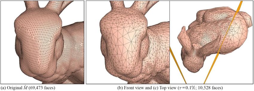
Adaptive Terrain Rendering using DirectX 11 Shader Pipeline                         Abstract

                                        Abstract

This thesis is about the development of a terrain rendering algorithm that uses the
DirectX 11 shader pipeline for rendering and the ability of DirectX 11 to render a
view-dependent level of detail system. The basics of terrain rendering and level of detail
systems are described and previous work that has been done on the subject of adaptive
terrain rendering is discussed. In addition, an explanation of the DirectX 11 shader
pipeline is provided. This shows how the new shader stages of the pipeline are
integrated to support hardware tessellation. Accordingly the developed algorithm will
be described and its usefulness for terrain rendering will be explored. Finally the
difficulties of the development will be mentioned and the future work will be discussed.

Keywords: thesis, terrain, view-dependent level of detail, tessellation, DirectX 11,
refinement, adaptive, hull shader, tessellator, domain shader

                                                                                i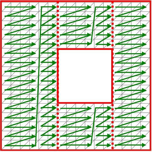
Adaptive Terrain Rendering using DirectX 11 Shader Pipeline           Declaration of originality

                    Declaration of originality

I hereby certify that I am the sole author of this thesis and that no part of this thesis has
been published or submitted for publication.
I certify that, to the best of my knowledge, my thesis does not infringe upon anyone’s
Copyright nor violate any proprietary rights and that any ideas, techniques, quotations,
or any other material from the work of other people included in my thesis, published or
otherwise, are fully acknowledged in accordance with the standard referencing
practices.

Markus Rapp, April 4, 2011

                                                                                    ii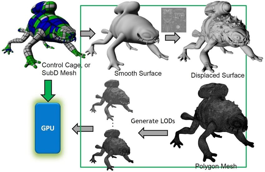
Adaptive Terrain Rendering using DirectX 11 Shader Pipeline           Acknowledgements

                            Acknowledgements

I want to say thank you very much for all people that supported me while I was writing
this thesis. A special thanks goes to my brother Daniel Rapp who supported me at the
last weeks of my thesis and gave me good advices so I could finish my work in time.
Also thank you very much for Michael Steele and Brigitte Bauer for supporting me with
their English skills. I would also like to say thank you to my parents who supported me
financially over my whole study time and helped me a lot so I could focus on my thesis.
Finally I want to say thank you to all professors and employees of “Hochschule der
Medien Stuttgart” that taught me a lot at my studies. Without the knowledge I got from
the lectures, making this thesis would not have been possible.

                                                                             iii
Adaptive Terrain Rendering using DirectX 11 Shader Pipeline                                                                                    Contents

                                                             Contents

Abstract .............................................................................................................................. i
Declaration of originality ................................................................................................ ii
Acknowledgements .......................................................................................................... iii
Contents ........................................................................................................................... iv
List of Figures ................................................................................................................. vi
1. Introduction.................................................................................................................. 1
2. Basics ............................................................................................................................ 3
   2.1. Coordinate System ........................................................................................................... 3
   2.2. Terrain Structure ............................................................................................................. 3
       2.2.1. Triangulated Irregular Networks ............................................................................................... 3
       2.2.2. Regular Grid .............................................................................................................................. 4
       2.2.3. Height Map ............................................................................................................................... 5

   2.3. Level of Detail ................................................................................................................... 7
       2.3.1. Discrete Level of Detail ............................................................................................................ 8
       2.3.2. Continuous Level of Detail ....................................................................................................... 9
       2.3.3. Distance-Dependent Level of Detail ....................................................................................... 11
       2.3.4. View-Dependent Level of Detail ............................................................................................ 12

   2.4. T-Junctions and Cracks................................................................................................. 16
3. Previous Work ............................................................................................................ 17
   3.1. ROAM ............................................................................................................................. 17
   3.2. Smooth View-Dependent Level-of-Detail Control and its Application to Terrain
   Rendering............................................................................................................................... 21
   3.3. Geometry Clipmaps ....................................................................................................... 26
4. DirectX 11 Shader Pipeline ....................................................................................... 31
   4.1. Input Assembler ............................................................................................................. 34
   4.2. Vertex Shader ................................................................................................................. 35
   4.3. Hull Shader ..................................................................................................................... 36
   4.4. Tessellator ....................................................................................................................... 37
   4.5. Domain Shader ............................................................................................................... 40
   4.6. Geometry Shader ........................................................................................................... 41
   4.7. Pixel Shader .................................................................................................................... 42

                                                                                                                                          iv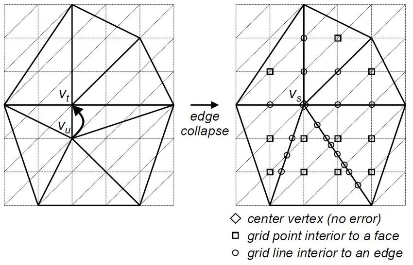
Adaptive Terrain Rendering using DirectX 11 Shader Pipeline                                                                                Contents

5. Terrain Rendering with DirectX 11 .......................................................................... 43
   5.1. Architecture of Terrain Engine .................................................................................... 43
   5.2. Implementation of View-Dependent Tessellation........................................................ 48
      5.2.1. Grid Construction .................................................................................................................... 48
      5.2.2. Normal calculation .................................................................................................................. 49
      5.2.3. Density Map Creation ............................................................................................................. 50
      5.2.4. Shader Pipeline ....................................................................................................................... 52

6. Conclusion.................................................................................................................. 58
   6.1. Future Work ................................................................................................................... 59
References ...................................................................................................................... 62

                                                                                                                                       v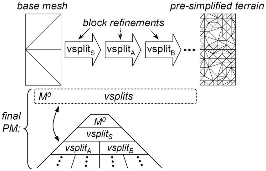
Adaptive Terrain Rendering using DirectX 11 Shader Pipeline                                                                    List of Figures

                                                List of Figures
Figure 2-1: Left-handed and right-handed Cartesian coordinate systems .................................................... 3

Figure 2-2: TIN representation [Gar95] ....................................................................................................... 4

Figure 2-3: Regular grid [Lue03] ................................................................................................................. 5

Figure 2-4: Gray scale height map with resolution 256 x 256 [AMD09] .................................................... 6

Figure 2-5: Color height map [Wig10] ........................................................................................................ 7

Figure 2-6: Different LODs of Stanford Bunny [Lue03] ............................................................................. 8

Figure 2-7: Different LODs of a quad [Lue03] ............................................................................................ 9

Figure 2-8: Shows edge collapse (ecol) and vertex split (vsplit) [Hop96] ................................................. 10

Figure 2-9: Progressive mesh [Hop96] ...................................................................................................... 10

Figure 2-10: Distance selection of Stanford Bunny LODs [Lue03] .......................................................... 11

Figure 2-11: Vertex hierarchy [Hop97] ..................................................................................................... 13

Figure 2-12: Shows modified edge collapse (ecol) and vertex split (vsplit) [Hop97] ............................... 14

Figure 2-13: Preconditions and effects of vertex split and edge collapse [Hop97] .................................... 14

Figure 2-14: Illustration of MA, MB and MG [Hop97]................................................................................ 15

Figure 2-15: View-dependent refinement example of Stanford Bunny [Hop97] ....................................... 16

Figure 2-16: Shows cracks and t-junctions [Lue03] .................................................................................. 16

Figure 3-1: Levels 0-5 of triangle binary tree [Duc97] .............................................................................. 17

Figure 3-2: Split and merge operation [Duc97] ......................................................................................... 18

Figure 3-3: Forced split of triangle T [Duc97]........................................................................................... 19

Figure 3-4: Construction of nested wedgies [Duc97] ................................................................................ 20

Figure 3-5: Changes to active mesh during forward motion of viewer [Hop98] ....................................... 22

Figure 3-6: Shows geomorph refinement [Hop981] .................................................................................. 23

Figure 3-7: Accurate approximation error [Hop98] ................................................................................... 23

Figure 3-8: Hierarchical block-based simplification [Hop98] ................................................................... 24

Figure 3-9: Result of the hierarchical construction process [Hop98] ........................................................ 25

Figure 3-10: Mesh with an average error of 2.1 pixels, which has 6.096 vertices [Hop98] ...................... 25

Figure 3-11: How geometry clip maps work [Asi05] ................................................................................ 26

Figure 3-12: Terrain rendering using a coarse geometry clipmap [Asi05] ................................................ 27

Figure 3-13: Terrain rendering using a geometry clipmap with transition regions [Asi05] ....................... 28

Figure 3-14: Illustration of triangle strip generation within a renderer region. [Los041] .......................... 29

                                                                                                                                    vi
Adaptive Terrain Rendering using DirectX 11 Shader Pipeline                                                                         List of Figures

Figure 4-1: Authoring pipeline of the past [NiT09] ................................................................................... 31

Figure 4-2: Real-time tessellation rendering [NiT09] ................................................................................ 32

Figure 4-3: Shader pipeline DirectX 11 ................................................................................................... 33

Figure 4-4: Input assembler ....................................................................................................................... 34

Figure 4-5: Vertex shader .......................................................................................................................... 35

Figure 4-6: Hull shader .............................................................................................................................. 36

Figure 4-7: Tessellator ............................................................................................................................... 37

Figure 4-8: Tessellation of a quad with tessellation factor 2.5 ................................................................. 38

Figure 4-9: Quads with different tessellation factors ................................................................................ 39

Figure 4-10: Domain shader ...................................................................................................................... 40

Figure 4-11: Geometry shader ................................................................................................................... 41

Figure 4-12: Pixel shader ........................................................................................................................... 42

Figure 5-1: Class diagram of terrain engine .............................................................................................. 43

Figure 5-2: Class diagram of CSystem ..................................................................................................... 43

Figure 5-3: Class diagram of CRenderer .................................................................................................. 45

Figure 5-4: Class diagram of CRenderable ............................................................................................... 46

Figure 5-5: How to create two triangles out of one quad ........................................................................... 49

Figure 5-6: Normal calculation .................................................................................................................. 49

Figure 5-7: Pixel selection and variation calculation for density map creation ......................................... 50

Figure 5-8: Calculation of variation .......................................................................................................... 51

Figure 5-9: Input and output of vertex shader ........................................................................................... 52

Figure 5-10: Vertex shader ....................................................................................................................... 52

Figure 5-11: Hull shader constant data, hull shader main function output and hull shader main function 53

Figure 5-12: Phong tessellation principle [Bou08] .................................................................................... 54

Figure 5-13: Domain shader ..................................................................................................................... 55

Figure 5-14: Terrain without tessellation ................................................................................................... 57

Figure 5-15: Terrain with tessellation ........................................................................................................ 57

Figure 6-1: Frame rate comparison with 256-to-256 height map (frame rate [rendered triangles]) .......... 58

Figure 6-2: Crack in terrain........................................................................................................................ 59

                                                                                                                                        vii
Adaptive Terrain Rendering using DirectX 11 Shader Pipeline                             1. Introduction

                                   1. Introduction

Terrain rendering has a wide application area. It has been used for virtual tourism,
education in subjects such as geography, for weather visualization, and to calculate the
most efficient positioning of radio, TV or cellular transmitter. Large companies such as
Google use terrain rendering for products like Google Earth.
Especially in the video games industry terrain rendering plays a big role as main
geometry for outdoor scenes. Open world games like Grand Theft Auto 4 or Mafia 2
were not be possible without a good terrain system. Also, for first person shooters
terrain is the main geometry for outdoor scenes. Game engines like Unreal Engine 3 and
Cry Engine 3 have their own terrain systems. Racing games use terrains for making the
tracks. Even dynamic terrain was used in games. One example is Sega Rally Revo
which was released in 2007 for PC, Xbox 360 and PS3. It uses a deformable terrain
system, which changes the course each lap. 1
What qualities and capabilities do we look for in a terrain renderer? A perfect terrain
would be a single continuous mesh from the foreground to the horizon with no cracks or
holes. A perfect terrain renderer would allow us to see a wide area over a large range of
detail. We want to walk on the terrain or fly over the terrain in real-time. To achieve
these requirements a rendering terrain algorithm has to be developed that has the ability
to blend out detail that is not seen or distant. This is done to save computing resources
to be able to show as much detail near the viewport as possible.
The first terrain renderer had a static geometry. Because of lack of these algorithms to
adapt geometry dependent on changing scene conditions it has always been necessary to
find a balance between small terrain with large detail and large terrain with less detail.

Since the 90’s a lot of research has been done about terrain rendering that supported a
greater level of detail (LOD). The main focus on development of these algorithms has
been to render a terrain in real-time that is as large as possible and has as much close up
detail as possible. 2

The first rendering algorithms that tried to achieve this target were CPU bound. The
final geometry was calculated on the CPU and send to the GPU for rendering. The GPU
only got the final data, which it had to render.
With the rapid development of graphics hardware the algorithms moved increasingly to
GPU. Therefore the algorithms had to be adapted to the specialized hardware to be
massively parallel.

1
    cf. http://www.gametrailers.com/video/preview-hd-sega-rally/26005 (accessed March 2011)
2
    cf. [Vir10], http://www.vterrain.org/LOD/Papers/ (accessed March 2011)

                                                                                              1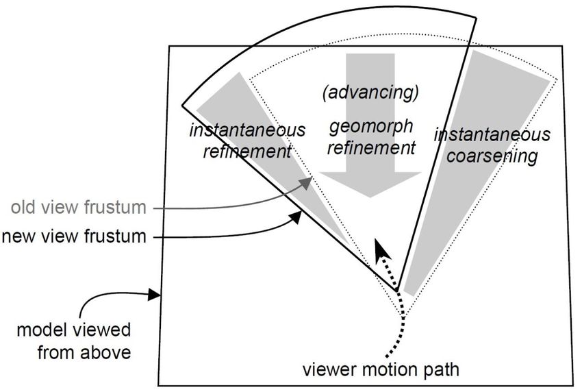
Adaptive Terrain Rendering using DirectX 11 Shader Pipeline                               1. Introduction

In 2005 ATI was the first company to integrate a hardware tessellator in their graphics
cards. With this tessellator it has been possible to refine the geometry entirely on the
GPU. ATI published a Tessellation SDK which made it possible to use the tessellator
together with DirectX9. 3

Two years later Microsoft released DirectX10 with Shader Model 4.0 which included
the new geometry shader. This made geometry refinement possible on all GPUs that
support DirectX 10.
The big break-through of hardware tessellation came with the introduction of
DirectX 11, which Microsoft released together with Windows 7 in 2009. DirectX 11
sets a standard for hardware tessellation with the new hull shader, tessellator and
domain shader. With this development, NVIDIA also decided to develop graphics cards
that are capable of tessellation.

The goal of this thesis is to develop a view-dependent LOD system. The main focus is
to develop a LOD system that is not visible for the user. It should show as much detail
as possible. Additionally an adaption of the detail should be possible in order that faster
hardware will show more detail than slower hardware. At the same time, the
development of the program should allow backward compatibility to older approaches.
This backward compatibility allows the use of old data. Terrain can also be rendered on
graphics cards that do not have a hardware tessellator integrated. The amount of visual
quality would be reduced, but the application could still run on older hardware.

In the end result it should also be possible to use a collision detection system or a
physics engine for the terrain. This would make it possible to walk over the terrain. All
this should be accomplished in real-time. For a fluid application it is important to have
at least 60 frames per second. In most applications terrain is only the base geometry.
Thus it would be better when a higher frame rate than 60 frames per seconds would be
achieved. Finally it should be developed a terrain editor that gives artists the ability to
model a terrain that uses the developed terrain rendering algorithm.
These goals will be attempted using the DirectX 11 shader pipeline with Shader Model
5.0. The hardware that is used for development is an AMD Radeon HD 6870.

The second chapter of the thesis will describe the basics of terrain rendering and level of
detail systems. In section 3 previous approaches to the topic will be discussed. The
following section is about the DirectX11 shader pipeline. Shader stages will be
explained. Section 5 will be shown the new developed tessellation terrain rendering
system. The final section will deal with the results of the new rendering system and
possible work for the future.

3
    cf. http://developer.amd.com/gpu/radeon/Tessellation/Pages/default.aspx (accessed March 2011)

                                                                                              2
Adaptive Terrain Rendering using DirectX 11 Shader Pipeline 2. Basics
2. Basics
In this section you’ll find some basic terms and definitions about terrain rendering.
Additionally you’ll read what exactly a LOD system is and which types of LODs exist.
2.1. Coordinate System
First it is important to decide which coordinate system to use. In Direct3D for example
it is possible to use a left-handed or right-handed Cartesian coordinates. Figure 2-1
shows the different coordinates.
Figure 2-1: Left-handed and right-handed Cartesian coordinate systems 4
In this thesis the left-handed Cartesian coordinates will be used. All explanations that
have to do with coordinates will be explained using left-handed Cartesian coordinates.
The x coordinate stands for length, y coordinate stands for height and z coordinate
stands for width.
2.2. Terrain Structure
The structure of a terrain can be differentiated in two major approaches, triangulated
irregular networks (TINs) and regular gridded height fields. Those two structures will
be described in the next two sections. 5
2.2.1. Triangulated Irregular Networks
A TIN constructs the terrain with a set of triangles dependent on the surface appearance.
Each vertex need to be stored. Figure 2-2 shows a terrain with 512 vertices. On the
4
cf. [Mic11], http://msdn.microsoft.com/en-us/library/bb204853%28v=vs.85%29.aspx (accessed March
2011)
5
cf. [Lue03], page 188
3Adaptive Terrain Rendering using DirectX 11 Shader Pipeline 2. Basics
lower right you see a part of the height field, which is flat. This part can be represented
with a few polygons. On the left side the surface is very bumpy. More polygons are
necessary to approximate the surface.
Figure 2-2: TIN representation [Gar95]
Advantages:
Surfaces can be approximated to the required accuracy. Large flat regions can be
represented with few polygons.
TINs are more flexible. Caves and overhangs can be constructed.
Disadvantages:
Irregularities of the surface make parallelization, collision detection, view-space
culling and dynamic deformations more complex.
TIN has a poor applicability for run-time view-dependent LOD.
TINs are not suitable for this analysis. The first reason is that parallelization is more
complex. This does not work for an approach that is mainly calculated on the GPU
because the architecture of a GPU is massively parallel. The second reason that makes
TINs impossible to use is that they are not applicable in a run-time view-dependent
LOD. Therefore TIN will not be used in this thesis. 6
2.2.2. Regular Grid
Regular or uniform grids are made out of quads. Each quad has the same size and
consists of two triangles. Grids are regularly spaced for length and width of the terrain.
The height of the terrain can be stored in an array or a height map.
In Figure 2-3 a regular gird of 8-to-8 is shown. It consists of 128 triangles.
6
cf. [Lue03], page 188 to 190
4Adaptive Terrain Rendering using DirectX 11 Shader Pipeline 2. Basics
Figure 2-3: Regular grid [Lue03]
Advantages:
X and z coordinates for width and length can be generated. Only the height
needs to be stored. Therefore less storage is needed.
Data can be stored in a texture. This is better for processing with GPU.
Regularity of the surface makes parallelization, collision detection, view-space
culling and dynamic deformations easier.
Disadvantages:
A grid has a less optimal representation and is unable to present different
complexity because same resolution is used over entire terrain.
It’s not possible to model overhangs or caves with a regular grid.
Grids are the perfect terrain structure for my requirements. All advantages are good for
less data storage and for parallel processing. The disadvantage to be not able to present
different complexities is not fatal because with tessellation it is possible to have
different resolutions. Of course the base grid is the lowest possible resolution. However,
over a million triangles will be rendered and the percentage of the possible number to
reduce when using another structure is so much less that it doesn’t need to be
considered. Also the disadvantage of not being able to model overhangs or caves is not
serious because there are other techniques like a Voxel Engine7 that can be used. 8
For these reasons I will use a regular grid as base structure for my algorithm.
2.2.3. Height Map
A height map is the best way to store height data for a regular grid. A height map is a
texture where the height data of a terrain is saved. There are four different approaches to
store the height data in a height map. One approach is to use the R-, G- and B-channel
7
cf. [Cry08], http://doc.crymod.com/SandboxManual/Voxel.html (accessed March 2011)
8
cf. [Lue03], page 188 to 190
5Adaptive Terrain Rendering using DirectX 11 Shader Pipeline 2. Basics
of a texture.9 In each channel the same data is stored. The result is a picture
representation of the heights in a gray scale. Figure 2-4 shows an example of such a
height map. This is nice for generating a height map. You can see on the texture how
the terrain will look like. Black stands for minimum height and white stands for
maximum height. However, the problem of this height map is its small data range. Only
256 different heights are possible. Therefore this type of height map is only good for
terrains that have a smaller difference in height. Another difficulty with this type of
height map is that 16 bit per pixel are wasted because the same data is saved in the R, G
and B channel of the texture.
Figure 2-4: Gray scale height map with resolution 256 x 256 [AMD09]
A second approach is to use a color height map. The representation of heights is now
displayed in colors. R, G and B channel of the texture are used for the height data. The
highest value is still white and the lowest value is black. With this approach 2 24
(16777216) different height values are possible. The advantage is that you still can
represent the different heights with colors in a picture. As well as in a gray scale height
map the alpha channel is free to use for additional data.
9
A texture has four channels: Red, Green, Blue and Alpha.
6Adaptive Terrain Rendering using DirectX 11 Shader Pipeline 2. Basics
Figure 2-5: Color height map [Wig10]
A third approach is to use the R and G channel for the height data. Now 65536 different
heights are possible. This is enough for the most applications. The B and Alpha channel
is still available for other data. The problem here is that you don’t have a picture
presentation of the heights. There have to be other ways to change the height data. One
approach could be to use a color height map at first to model a height map in a 2D
texture view. After this the height data is converted to the 16 bit to fit in the R and G
channel.
It is also possible to use all channels of a texture for height data. With this 232 height
values are possible. 10 11
The advantages of height maps are that they are easy to implement and require
substantially less memory than a polygon mesh representation. Furthermore GPUs are
specialized to access textures. So a height map is also a good data representation for a
GPU.
2.3. Level of Detail
In computer graphics level of detail is a technique that is concerned with the reduction
of complexity of 3D polygon models. This reduction of complexity is done for the
purpose of decreasing the workload of graphics hardware to be able to show more detail
where it is needed.
The necessary polygon count of an object depends on the shape of an object as much as
on the distance and orientation of the object to the camera. The used screen resolution is
a dependency for the polygon count, as well. A level of detail system tries to calculate a
representation of a polygon object according to these dependencies.
10
cf. [Sch06], page 756
11
cf. [Wig10], page 308, 309
7Adaptive Terrain Rendering using DirectX 11 Shader Pipeline 2. Basics
There are several different approaches of level of detail systems.
2.3.1. Discrete Level of Detail
Discrete LOD is a scheme where several discrete models with fewer triangles are
calculated or modeled for a complex model. The different models are precomputed
offline and can then be used inside the application when they are needed. At run-time
the application chooses which representation of the model is best suited to the scene
conditions and should be rendered.
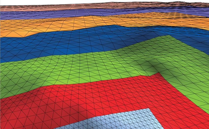
Discrete LOD is also called view-independent LOD. When the LODs are computed it
can’t be predicted in which direction the camera shows.
In Figure 2-6 you see how the different LODs of a model could look like.
Figure 2-6: Different LODs of Stanford Bunny [Lue03]
Advantages:
Decoupling simplification and rendering makes it good for real-time
applications. Expensive precomputation for precise LODs can be made offline.
At real-time not much processing power is needed.
It is very simple at run-time. Only the model needs to be switched.
Disadvantages:
Additional memory is needed to store each representation of the model.
Switching between different LODs is visible for the user because of the little
number of LODs.
Discrete LODs are not dependent on viewing direction.
Discrete LODs are applicable for applications that don’t have much compute power.
But using a discrete LOD system also means a poorer visual quality.
In a terrain system you would have a grid with different quad sizes. Some quads of the
grid would be very small for a high resolution and some quads of the grid would be very
large. Figure 2-7 shows different resolutions of a quad. The sizes of the quads would be
8Adaptive Terrain Rendering using DirectX 11 Shader Pipeline 2. Basics
selected according to the scene conditions. Because there are only a discrete number of
quad sizes, the user would see a change of shape of the terrain when one quad size
changes to a lower or higher quad size. 12
Figure 2-7: Different LODs of a quad [Lue03]
2.3.2. Continuous Level of Detail
Continuous LOD is completely different to discrete LOD. Rather than have some
discrete LOD models, continuous LOD defines a continuous spectrum of data detail.
This spectrum reaches from a low polygon mesh to a high polygon mesh. All you need
for this is a low poly mesh and a data structure that defines how this mesh can be
refined. According to this structure a mesh can be created on run-time that fits to the
scene conditions.
Advantages:
Continuous LOD has a better granularity because the number of possible meshes
with different LODs is much higher than with discrete LOD.
The better granularity leads to a better fidelity. An exact model can be created,
and only the number of polygons that are essential will be created.
The better granularity also leads to a smoother transition because the difference
between the possible LOD meshes is very small.
Streaming of the refinement data is possible.
Disadvantages:
Continuous LOD is much more complex.
More processing is needed at run-time.
In conclusion, continuous LOD offers a much better visual representation with the cost
of additional computation. 13 14
An example for a continuous LOD is the progressive mesh representation that was
presented from Hugues Hoppe on ACM SIGGRAPH 1996. The progressive mesh
representation works with two operations, edge collapse (ecol) and vertex split (vsplit).
12
cf. [Lue03], page 5, 9, 334
13
cf. [Lue03], page 10, 332
14
cf. [Red03], [Lue031]
9Adaptive Terrain Rendering using DirectX 11 Shader Pipeline 2. Basics
Figure 2-8 shows how these operations are performed. For edge collapse you have four
vertices Vl, Vr, Vt and Vs. Vt and Vs are unified into to one vertex Vs. Vertex split is the
reverse of this operation. It splits Vs into two vertices Vt and Vs.
Figure 2-8: Shows edge collapse (ecol) and vertex split (vsplit) [Hop96]
But how are these operations used to make a continuous LOD? First we need to model a
high polygon mesh Mn. Next we define a sequence of edge collapses that simplify Mn to
a very coarse mesh M0. After this we have a spectrum that reaches from n to 0 where
each step is one edge collapse.
An edge collapse transformation is invertible with a vertex split. When we invert the
previous process, we can start with the base mesh M0 and make vertex split operations
until we get to the high poly mesh Mn. Now we have a spectrum from 0 to n where each
step is a vertex split.
Figure 2-9 shows four models of a spectrum, which consists of 13369 different
models.15 In an application we use the low polygon mesh M0 and a sequence vertex
splits. According to the distance to the camera we now refine or coarse our model with
edge collapse and vertex split operations. 16
Figure 2-9: Progressive mesh [Hop96]
15
M0 = 150 faces, MN = 13546 faces; number of possible meshes = (MN-M0)/2 = 13369
16
cf. [Hop96] [Hop961]
10Adaptive Terrain Rendering using DirectX 11 Shader Pipeline 2. Basics
Progressive meshes alone are not applicable for a terrain system. Because we have only
one refinement sequence, the terrain only can be refined at one part of its surface. One
sequence is enough for a small mesh but for a big terrain it is insufficient.
2.3.3. Distance-Dependent Level of Detail
Distance-dependent is the selection of LODs dependent on the distance between the
camera and the rendered object. This selection criterion can be applied to a discrete
LOD or a continuous LOD system. In Figure 2-10 you see an example how the
Stanford Bunny LODs are rendered according to the distance of the camera.
Figure 2-10: Distance selection of Stanford Bunny LODs [Lue03]
When selecting a LOD it is important to use the true 3D distance instead of the distance
between camera and object in view-space after projective transformation. It’s common
in a 3D game or application to rotate the camera rapidly. This rapid rotation of the
camera would lead in a screen depth based LOD selection to changes of LOD models,
which could lead to visual artifacts.
It is advisable to use tolerance factors like hysteresis to avoid LOD changes resulting
from small changes in viewer distance. Hysteresis is a lag between LOD transitions so
that objects switch to a lower LOD slightly further away than the defined distance and
to a higher LOD at a slightly closer distance. For example if we have a distance of 100
to the camera where we switch from LOD1 to LOD2. Now we define a threshold 10 for
the hysteresis. We would switch from LOD1 to LOD2 at 110 and LOD2 to LOD1 at 90.
So the range between 90 and 110 is where both LODs could appear. When moving
away from the object it is the LOD1 and when moving towards the object it is the
LOD2.
Advantage:
Distance-dependent LOD is simple and efficient to implement. Only the distance
in 3D space between two points needs to be calculated.
11Adaptive Terrain Rendering using DirectX 11 Shader Pipeline 2. Basics
Disadvantages:
Only using the distance for LOD selection is inaccurate because shape or
orientation of the mesh to the camera are not considered.
View-distance conditions can change when scaling a mesh or using different
display resolutions.
In conclusion, distance-dependent LOD is the best selection for discrete LOD and
continuous LOD because the different LODs of the schemes only depend on the
distance to the camera. 17
In section 3.3 a terrain rendering approach is described that uses distance-dependent
LOD for its LOD selection.
2.3.4. View-Dependent Level of Detail
View-dependent LOD is an extension of continuous LOD. The selection of LOD is
done with view-dependent selection criteria such as screen resolution, orientation of the
camera and shape of a polygon mesh. Meshes that are near to the camera have a higher
detail than meshes that are far away.
The human visual system is sensitive to edges. Therefore a view-dependent LOD
system also provides to have a higher detail on silhouette regions and less detail on the
interior regions of a mesh.
One major problem of continuous LOD is that either we have a very detailed mesh or a
very coarse mesh. A view-dependent LOD provides the ability to have a mesh that on
the one hand has very detailed parts like silhouette of the mesh or parts that are really
near to the camera. On the other hand the same mesh could also have some regions of
the mesh that are not that detailed. These parts are in the interior region of the mesh or
parts that are not that close to the camera. There are also some parts of the mesh that are
not seen from the user such as faces oriented to the rear or parts that are outside the
view frustum. These parts that are not seen should not be rendered.
Advantages:
A view-dependent LOD system provides even better granularity than a
continuous LOD system. The outcome of the better granularity is a higher
fidelity. As a result polygons are allocated exactly where they are needed.
View-dependent LOD provides smoother transition between LODs. This leads
to a reduction of popping effects18 that plague discrete LOD.
Drastic simplification of very large objects is possible.
17
cf. [Lue03], page 88-90, 93-94, 180
18
Popping effect is the noticeable flicker that can occur when the graphics system switches between
different LODS. cf. [Lue03], page 342
12Adaptive Terrain Rendering using DirectX 11 Shader Pipeline 2. Basics
Disadvantage:
Relatively high computational cost at run-time.
View-dependent LOD seems to be the perfect approach to have the best visual quality
with fewest polygons. The only problem is the high computational cost at run-time that
comes with view-dependent LOD. 19 20
An example for a view-dependent LOD is “View-Dependent Refinement of Progressive
Meshes”. This is a further development of progressive meshes and was developed by
Hugues Hoppe. With this approach different LODs can coexist on one mesh. Regions
that are outside the view frustum, distant or facing away from the camera are coarsened.
With progressive meshes vertex split and edge collapse operations are only possible in a
defined sequence. Therefore it is not possible with this technique to have different
LODs on one mesh. To define different LODs on one mesh we need to be able to make
vertex split and edge collapse operations on several parts of the mesh. The first thing we
need to be aware of is that a vertex split transformation defines a parent-child
relationship between the vertex Vs that gets split and the new created vertices Vt and Vu.
This parent-child relation can be applied to a binary tree.
Figure 2-11 shows how such a vertex hierarchy of vertex splits is constructed. In this
example we got a coarse mesh M0 that has three vertices V1, V2, V3. Each of these
vertices can be split independently of the other vertices. With a vertex split two new
child nodes are created. As a result of all vertex splits we got M^, which consists of all
child nodes. With this vertex hierarchy we can now make selectively vertex split and
edge collapse operations. We don’t have a defined sequence anymore. But we still have
some restriction. We are not able to split and collapse any part we want.
Figure 2-11: Vertex hierarchy [Hop97]
19
cf. [Lue03], page 10-12, 104
20
cf. [Lue031]
13Adaptive Terrain Rendering using DirectX 11 Shader Pipeline 2. Basics
But what are the restrictions? Before I talk about the restriction for vertex split and edge
collapse I need to introduce the modified vertex split and edge collapse operations. The
operations where modified because with the old operations it was not possible to define
a consistent restriction for edge collapse. Figure 2-12 shows the new operations. For a
vertex split we need to consider the four neighboring faces fn0, fn1, fn2 and fn3 of vertex
Vs. A vertex split now creates two new vertices Vu and Vt. It also creates two new faces
fl and fr, which are surrounded of the faces fn1, fn2, fn3 and fn4. An edges collapse
transformation has the same parameters as a vertex split operation and performs the
inverse operation.
Figure 2-12: Shows modified edge collapse (ecol) and vertex split (vsplit) [Hop97]
There are new restrictions that come with these operations. A vertex split operation is
legal if Vs is active and fn0, fn1, fn2, fn3 are active. A vertex or a face is active if it exists
in the selectively refined mesh MS. For example in Figure 2-11 vertices V1, V2, V3 are
active in M0. An edge collapse is legal if Vt, Vu are active and if the faces to fi and fr are
adjacent to fn0, fn1, fn2, fn3. Figure 2-13 demonstrates these preconditions.
Figure 2-13: Preconditions and effects of vertex split and edge collapse [Hop97]
Now that we have the algorithm to refine the mesh we only need to define the criteria
that tell us when to refine the mesh. There are three criteria. The mesh only will be
14Adaptive Terrain Rendering using DirectX 11 Shader Pipeline 2. Basics
refined if the surface is inside the view frustum, faces the viewer or if screen-space
geometric error exceeds screen-space tolerance τ. The screen-space tolerance can be
adapted according to refinement level that wants to be achieved. A byproduct of the
screen-space geometric error is that the refinement is denser near the silhouettes and the
mesh is coarser the farther it is from the viewpoint.
The selective refinement framework also supports geomorphs. Geomorphs make a
smooth transition between two selectively refined meshes possible. MA and MB are two
selective refined meshes. MG is a selective refined mesh whose active vertex front is
everywhere lower or equal then the active vertex front of M A or MB. By interpolating
the vertices of MG, it’s possible to make a smoothly transition between MA and MB.
Figure 2-14 shows an example of MA and MB with the corresponding MG.
Figure 2-14: Illustration of MA, MB and MG [Hop97]
The presented algorithm exploits frame coherence. The mesh of the last frame is
adapted to fit to the next frame. Therefore, small changes in the view are good for this
algorithm. Bad for this algorithm are fast camera rotations or rapid movement. The
algorithm is efficient. It needs about 15% of frame time. Additionally it is possible to
reduce the overhead of this algorithm by considering each frame only a fraction of the
active vertex list that leads to a delay of the detail adaption of the mesh.
Figure 2-15 shows how selected refinement is used for a mesh with 69473 faces. In this
view it is possible to reduce the face number to 10582 using a screen-space tolerance of
0.1. This is a reduction of about 85% of the faces of the original mesh. 21 22
A modified version of this algorithm was used for terrain rendering. This approach will
be explained in section 3.2.
21
cf. [Hop97]
22
cf. [Hop971]
15Adaptive Terrain Rendering using DirectX 11 Shader Pipeline 2. Basics
Figure 2-15: View-dependent refinement example of Stanford Bunny [Hop97]
2.4. T-Junctions and Cracks
There is one common problem when using different LODs on one grid. Adjacent
triangles with different LODs are not connected properly when the higher LOD has a
vertex that does not share a vertex of the lower LOD. This phenomenon is called
t-junction. This t-junction could lead to bleeding tears in the terrain.
If additionally the vertex of the higher LOD doesn’t lie on the edge of the lower LOD
cracks will appear. These cracks lead to holes in the terrain.
Figure 2-16: Shows cracks and t-junctions [Lue03]
The solution of this problem is to have LODs that share the same vertices on the
adjacent edges. How this is implemented is dependent on the LOD system that is used.
Therefore I will explain how t-junctions and holes are avoided when I write about the
terrain LOD systems. 23 24
23
cf. [Sch06], page 757
24
cf. [Lue03], page 193
16Adaptive Terrain Rendering using DirectX 11 Shader Pipeline 3. Previous Work
3. Previous Work
In this section three previous terrain rendering algorithms will be explained.
3.1. ROAM
ROAM stands for real-time optimally adapting meshes. In 1997 it was developed in
cooperation of Los Alamos National Laboratory and Lawrence Livermore National
Laboratory. The algorithm was very popular among game developers and has been
implemented for Tread Marks, Genesis3D and Crystal Space engine. ROAM has
view-dependent error metrics, is able to achieve specified triangles counts and uses
frame-to-frame coherence.
Figure 3-1: Levels 0-5 of triangle binary tree [Duc97]
The base idea of ROAM is to use a right-isosceles triangle T. This triangle has three
vertices V0, V1 and Va. The edge between V0 and V1 is the hypotenuse of the triangle.
Va is the apex of the triangle. To split T, a new edge is built from Va to a new vertex Vc,
which is in the middle of the hypotenuse of T. The result is two new vertices T 0 and T1,
which have the same size. This split can recursively performed until the necessary
17Adaptive Terrain Rendering using DirectX 11 Shader Pipeline 3. Previous Work
refinement is achieved. This approach works for terrain rendering because a quad of a
regular grid consists of two right-isosceles triangles.
Figure 3-1 shows the first six levels of a triangle binary tree. In level 5 the triangle
count is 32 triangles. ROAM uses a triangle binary tree structure to keep track of the
refinement scale of each triangle. As mentioned in section 2.4 when dealing with
different LODs, t-junctions could be a problem. This is a problem of this approach as
well. To avoid this t-junctions ROAM stores for each node its left child T0, right child
T1, left neighbor TL, right neighbor TR and its base neighbor TB. Additionally TB of T
has to have the same LOD level. TL and TR of T either have to be from the same LOD
level, from the next finer level or from the next coarser level. Taking these restrictions
into account we need to split TB when we want to split T. This split is called diamond
split. The reverse of a split operation is called merge. Every split operations are totally
reversible. See Figure 3-2 for a graphical representation of split and merge. On the left
side you see a typical neighborhood for T. TL, TR and TB are from the same LOD level
and also the neighboring triangles of TB fulfill the requirements. So a diamond split can
be performed, which creates the four new triangles T0, T1, TB1 and TB0.
To provide a smooth transition splits and merges can be animated by using vertex
morphing. Instead of just adding a new vertex Vc as shown in Figure 3-1, we could
create Vc on the position of Va and then move Vc over time to its final position.
Figure 3-2: Split and merge operation [Duc97]
But what to do when neighboring triangles of T don’t fulfill the conditions? If this
happens the neighboring triangles need to be forced split or forced merged. Figure 3-3
shows an example where TB has one coarser level than T. To be able to split T, TB
needs to be split first. This is not possible because the base neighbor of TB is from a
coarser level as well. So a forced split is performed recursively on the base neighbor
until a diamond is found, where a triangle has the same LOD level as its base triangle.
18Adaptive Terrain Rendering using DirectX 11 Shader Pipeline 3. Previous Work
Now diamond splits can be made until T is split. In the case of Figure 3-3 four diamond
splits are required to split T.
Figure 3-3: Forced split of triangle T [Duc97]
To take advantage of frame coherence, ROAM uses a dual queue approach, the split
queue and the merge queue. According to the importance of the split or merge these
queues are sorted. The most imported merges and splits are performed first. This gives a
good flexibility at run-time. In a frame coherence system the amount of splits and
merges are dependent on the change of the viewport. If the change of the viewport is big
the system needs to do a lot of merges and splits. This could lead to a drop in the frame
rate. With the two priority queues it is now possible to do only the most important
calculations in the queue and do the rest in another frame where the change is not that
big. So a constant frame-rate can be guaranteed while having only a small error.
The base error metric of ROAM is to calculate the distance between where the surface
point should be in screen space and where the triangulation places the point. Therefore
nested world-space bounds are needed. These are precalculated bounding volumes
around each triangle, which were calculated in world space and are called wedgies. The
wedgies allow faster calculation and provide a guaranteed error bound. This error bound
is the maximum amount that the plane formed by the triangle varies from the original
fine detailed terrain. Figure 3-4 shows how wedgies are built through the vertices when
a merge operation is done. At real-time the precalculated wedgies are transformed into
screen space to compute a local upper bound, which represents the base error metric.
Other most important error metrics that can be done with ROAM are back-face detail
reduction, view frustum and silhouette edges. For all triangles that are facing away from
the camera and outside the view frustum the priority can be set to a minimum. Because
the viewer doesn’t see these triangles they can be coarsened in a later frame without the
19Adaptive Terrain Rendering using DirectX 11 Shader Pipeline 3. Previous Work
viewer recognizing it. Silhouette edges are the triangles, where a front-face to back-face
transition takes place. To have a good visual representation, it is important to give such
triangles a high priority.
Figure 3-4: Construction of nested wedgies [Duc97]
Now that we have all building blocks of ROAM we can look at the processing phases
that are performed each frame.
1. View frustum culling is updated.
2. Do priority update for triangles that can potentially be split or merged in next
phase. Split queue and merge queue is updated.
3. Triangulation update driven by split and merge queue.
4. Update all triangles that area dependent on phase 1 and 3.
One limitation for terrain rendering is important to mention. The resolution of the height
map is the limitation for the level of refinement of the terrain. So the maximum detail of
the terrain is directly dependent of the size of the height map. Therefore the refinement
of a triangle stops when either the error is small enough or the maximal triangle count is
reached.
In conclusion ROAM is a flexible view-dependent terrain rendering algorithm, which
allows a fixed frame rate and can work towards a fixed triangle count. The problem
with ROAM is that it makes small sets of triangles for rendering. Modern GPUs are
working better with a large number of triangles. Because of that ROAM 2.0 was
20Adaptive Terrain Rendering using DirectX 11 Shader Pipeline 3. Previous Work
developed which mixes the continuous LOD approach of ROAM with a discrete LOD
system. 25 26
The original ROAM algorithm has been modified and improved by a number of
researchers and game developers. One example is the implementation of Bryan Turner.
He implemented a simplified version of ROAM. In his approach he uses a split only
approach where the terrain is refined from scratch in each frame. Therefore he uses a
variance binary tree, which stores geometric error. The variance tree is updated every
frame according to the change of the scene. The terrain is then tessellated according to
the variance binary tree. 27
ROAM is also able to deal with dynamic terrain. Yefei He developed a real-time
dynamic terrain for an off-road ground vehicle simulation, in which a vehicle can
deform the terrain. So it’s possible to form skid marks of the car into the terrain. The
system is called DEXTER (Dynamic EXTEnsion of Resolution). 28
3.2. Smooth View-Dependent Level-of-Detail Control and its
Application to Terrain Rendering
Hugues Hoppe developed the terrain algorithm in 1998. The representation uses as base
view-dependent progressive meshes that were introduced in section 2.3.4. The target of
this terrain rendering systems was to render the Grand Canyon data in real-time, which
has about 16.7 million triangles. To be able to render this data the complexity of the
terrain needed to be reduced to 20000 triangles. This was the number of polygons,
which graphics hardware was able to render in 1997. To achieve this target they would
like to adapt the mesh complexity according to the screen-space projected error, which
makes a view-dependent LOD system. So the terrain is refined more densely near the
viewer, while distance and regions outside the view frustum are kept coarser. It was also
the goal to make a terrain rendering system with improved approximation error and that
provides scalability. Two important factors for a good terrain system they also tried to
achieve were a constant frame rate and the absence of popping artifacts.
To avoid popping artifacts the screen-space error value needs to be near 1 pixel. When
the screen-space error is near 1 pixel the change of resolution can’t be seen by the
viewer. The problem of a constant error tolerance is that the number of faces depends
directly on the terrain complexity near the viewpoint. This leads to a non-uniform frame
rate because the frame rate is dependent on the number of triangles that need to be
25
cf. [Duc97]
26
cf. [Lue03], page 202-206
27
cf. [Tur00]
28
cf. [HeY00]
21Adaptive Terrain Rendering using DirectX 11 Shader Pipeline 3. Previous Work
rendered, and these are not constant in this approach. For a constant frame rate, the
screen-space error needs to be adjusted. But this leads to popping artifacts. To hide the
popping artifacts they use geomorphs. At run-time the triangles of the terrain need to be
split or refined to get the needed resolution. Instead of doing the refine and split in one
frame they morph it over several frames.
When do we need to use this geomorphing in a terrain rendering system? There are two
different situations we need to consider. One is forward moving the other is backward
moving.
When we move forward we use geomorph refinement. In Figure 3-5 we see how the
view port changes when we move forward and turn left at the same time. We get three
different regions. All parts that are new in the view frustum are instantaneous refined,
all parts that are outside the view frustum are instantaneous coarsened and all parts that
were visible in the frame before, we need to do geomorph refinement.
Figure 3-5: Changes to active mesh during forward motion of viewer [Hop98]
Figure 3-6 shows how a geomorph refinement is done. At first we do a split operation.
But instead of placing the new created vertex directly on its final position we spawn the
vertex on the old vertex. After this we move the new vertex over several frames to his
new position. How long this morphing takes, depends on a user specified time, which is
called gtime. With a frame rate between 30 to 72 fps the gtime is set to 1 second. A nice
thing about geomorph refinement is that while a new vertex is morphing it can be split
already. So we’re able to do several geomorph refinements at the same time.
22You can also read