INDIAN OCEAN DECADAL VARIABILITY - A Review
←
→
Page content transcription
If your browser does not render page correctly, please read the page content below

INDIAN OCEAN
                        DECADAL VARIABILITY
                                                          A Review
                           by   Weiqing Han, Jérôme Vialard, Michael J. McPhaden, Tong Lee,
                                 Yukio Masumoto, Ming Feng, and Will P.M. de Ruijter

          Improved definition and understanding of decadal timescale variability in the Indian Ocean region
          will support climate prediction efforts and have the potential to benefit a large percentage of the
                world’s population living in Indian Ocean rim countries and elsewhere around the globe.

    E
         xisting records of upper-ocean temperature                    by natural external forcing, such as volcanic eruptions
         exhibit clear fluctuations at time scales ranging             and variability in solar forcing (e.g., Domingues et al.
         from one to a few decades, which for simplicity               2008), and part of which is due to natural internal
    we refer collectively to as “decadal variability” in this          variability (e.g., Meehl et al. 1998; Alexander 2010; Liu
    paper1 (see Fig. 1). This variability includes a rising            2012). In view of society’s need for adapting to climate
    trend since the 1960s, which is attributed to anthro-              variability and change, understanding and predicting
    pogenic greenhouse gas forcing, with about 90% of                  climate on decadal time scales emerge as pressing
    the excess heat input in the climate system stored in              priorities in climate research today (Goddard et al.
    the ocean (Levitus et al. 2012). Overlying this trend              2009; Hurrell et al. 2009; Meehl et al. 2009; Pohlmann
    are decadal fluctuations, part of which may be caused              et al. 2009; Doblas-Reyes et al. 2011). Preliminary

Fig. 1. Time series (1955–2012) of yearly, ocean heat content (1022 J) for the 0–700-m layer of the Indian Ocean
(thick solid curves). One standard deviation errors (thin vertical lines) and linear trends (dotted lines) are shown
in each panel. Data provided by Dr. John Antonov and replotted after Levitus et al. (2009).

    1
        Unless specified otherwise in this review, “decadal” variability will refer broadly to variations on decadal to multidecadal
        time scales, spanning 10–100 yr.

    AMERICAN METEOROLOGICAL SOCIETY                                                                       NOVEMBER 2014            | 1679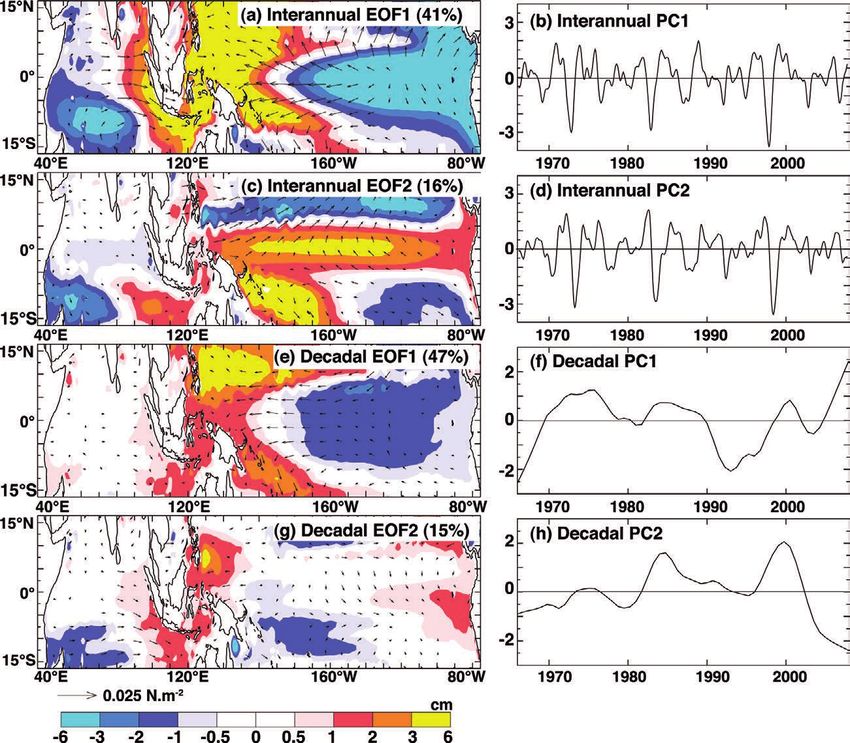
decadal prediction experiments have been carried                    SanchezGomez et al. 2008; Schott et al. 2009) and
      out and assessed recently (e.g., Collins 2002; Smith                North Pacific (e.g., Chen et al. 1992; Graham et al.
      et al. 2007, 2013; Keenlyside et al. 2008; Hoerling                 1994; Deser and Phillips 2006). Progressive warming
      et al. 2011; Corti et al. 2012). Defining the limits of             of Indian Ocean SST also influences the tropical
      decadal predictability and developing models capable                atmospheric circulation by strengthening the Pacific
      of skillful decadal predictions, however, rely critically           Walker circulation (Luo et al. 2012), which intensifies
      on our understanding of the causes of decadal vari-                 the easterly trade winds and thereby accelerates sea
      ability, including contributions from both external                 level rise in the western tropical Pacific Ocean (Han
      forcing (greenhouse gases, aerosols, volcanoes, and                 et al. 2014). Air–sea coupling over the tropical Indian
      solar forcing) and natural internal variations of the               Ocean can induce large-amplitude decadal modula-
      climate system (e.g., Hoerling et al. 2011; Solomon                 tions of El Niño–Southern Oscillation (ENSO; Yu
      et al. 2011).                                                       et al. 2002; Yu 2008) and of the relationship between
          While natural modes of decadal climate vari-                    ENSO and the Indian monsoon (Ummenhofer et al.
      ability have been identified and extensively studied                2011). Decadal variations of Indian Ocean SST have
      in the Atlantic and Pacific Oceans [see reviews by                  led to an intensification of Arabian Sea premonsoon
      Alexander (2010) and Liu (2012)], decadal variability               tropical cyclones in recent decades (Rao et al. 2008;
      of the Indian Ocean is much less understood. There                  Krishna 2009; Evan et al. 2011; Sriver 2011; Wang et al.
      is, however, considerable evidence showing that                     2012). The decadal trend in upper-ocean heat content
      Indian Ocean decadal sea surface temperature (SST)                  in the southeast Indian Ocean combined with the
      variations have large climate impacts both regionally               strong 2010/11 La Niña forced an extraordinary surge
      and globally.                                                       of the Leeuwin Current off the west coast of Australia
          Both observational and modeling studies have                    during austral summer 2011. This surge resulted in
      shown that decadal variability in Indian Ocean                      an unprecedented warming event (recently dubbed
      SST can inf luence the tropical and extratropical                   Ningaloo Niño) in February–March 2011 (Feng et al.
      atmosphere via changes in the Walker and Hadley                     2013; Kataoka et al. 2013), which had devastating im-
      circulations (Wang and Mehta 2008) and in particular                pacts on living marine resources in the region (Pearce
      impact weather regimes and climate variability in                   and Feng 2013).
      the North Atlantic (Bader and Latif 2005; Hoerling                      Tropical Indian Ocean SST variations have large
      et al. 2004; Hurrell et al. 2004; Latif et al. 2006;                climatic impacts over continents as well. Indian
                                                                          Ocean warming acted in concert with tropical
                                                                          Pacific cooling to force droughts over the United
AFFILIATIONS: Han —Department of Atmospheric and Oceanic                  States, southern Europe, and southwest Asia during
Sciences, University of Colorado, Boulder, Boulder, Colorado;             1998–2002 (e.g., Hoerling and Kumar 2003; Lau
Vialard —Laboratoire d’Océanographie: Expérimentation et                  et al. 2006). The Indian Ocean warming trend may
Approches Numériques, IRD, CNRS, MNHN, Université Paris 6,                have contributed to the increased frequency of
Paris, France; McPhaden —NOAA/Pacific Marine Environment
                                                                          Mediterranean winter drought during the past 20 yr
Laboratory, Seattle, Washington; Lee —Jet Propulsion Laboratory,
                                                                          (Hoerling et al. 2012), to the drying trend over West
California Institute of Technology, Pasadena, California;
Masumoto —Climate Variation Predictability and Applicability              Sahel from the 1950s to the 1990s (Bader and Latif
Research Program, Japan Agency for Marine-Earth Science                   2003, 2005; Giannini et al. 2003; Lu 2009; Mohino
and Technology, Yokohama, Japan; Feng —CSIRO Marine and                   et al. 2011), and to the drier eastern Africa “long-rain”
Atmospheric Research, Center for Environment and Life Sciences,           season since 1980 (Williams and Funk 2011). Indian
Floreat, Western Australia, Australia; De Ruijter—Institute for           Ocean SST also controls multidecadal variability in
Marine and Atmospheric Research, Utrecht University, Utrecht,             the hydroclimatic conditions of East Africa (Tierney
Netherlands
                                                                          et al. 2013). In addition, the reduced interhemispheric
CORRESPONDING AUTHOR: Weiqing Han, Department of
Atmospheric and Oceanic Sciences, University of Colorado,
                                                                          SST gradient associated with the aerosol loading of
Boulder, UCB 311, Boulder, CO 80309                                       the atmosphere from South Asia since the 1950s acts
E-mail: weiqing.han@colorado.edu                                          to weaken the Indian summer monsoon rainfall
                                                                          (Chung and Ramanathan 2006; Meehl et al. 2008;
The abstract for this article can be found in this issue, following the
table of contents.
                                                                          Dash et al. 2009).
DOI:10.1175/BAMS-D-13-00028.1                                                 The Indian Ocean rim region is home to one-
                                                                          third of the world’s population, mostly living in
In final form 6 March 2014
©2014 American Meteorological Society                                     developing countries that are highly vulnerable to
                                                                          climate variability and change, especially in low-

1680 |          NOVEMBER 2014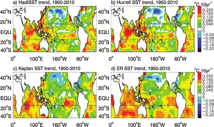
lying coastal areas. Indian Ocean island nations are           is to summarize the observational basis for, and our
     likewise vulnerable to the vicissitudes of climate,            current understanding of, decadal variability in the
     including the likely increased incidence and/or                Indian Ocean. We will also identify outstanding sci-
     magnitude of extreme high sea level events (Rhein              entific issues that need to be addressed and challenges
     et al. 2014). Consequently, there is a strong societal         we face in addressing them.
     demand for improved understanding and prediction                   In the section titled “Indian Ocean circulation and
     of decadal climate variability and sea level rise in the       interannual climate variations,” we briefly review
     region (Milne et al. 2009; Church et al. 2011). Yet,           the mean circulation and interannual variability of
     our knowledge about Indian Ocean decadal vari-                 the Indian Ocean, since these concepts are helpful
     ability remains primitive compared to the Pacific and          for describing decadal variability in later sections.
     Atlantic Oceans. The purpose of this review therefore          In the section titled “observed decadal variability

UNCERTAINTIES IN TRENDS OF THE INDO-PACIFIC WALKER CIRCULATION.

T  he Walker circulation is an equatorial
   zonal atmospheric circulation cell,
driven by deep atmospheric convec-
                                               1950s and 1960s (Han et al. 2010; Yu
                                               and Zwiers 2010; Yasunaka and Kimoto
                                               2013), while the bias-corrected observed
                                                                                          Sea Surface Temperature dataset,
                                                                                          version 3 (HadSST3; Kennedy et al.
                                                                                          2011a,b) produces a weakened Walker
tion over the Indo-Pacific warm pool           winds indicate a weakening of equato-      circulation. If HadSST3 is the best
(Fig. SB1). The lower branch of the            rial Indian Ocean surface westerlies       dataset for detecting tropical Indo-
Walker circulation is associated with          (Tokinaga and Xie 2011; Tokinaga et al.    Pacific SST changes, then the Indo-Pacific
easterlies in the Pacific Ocean and            2012a,b).                                  Walker circulation should be weakening.
westerlies in the Indian Ocean that are            Modeling studies also provide con-     Without a careful investigation and com-
important for driving decadal variations       trasting results. Coupled global climate   parison of data processing and analysis
in the Indian Ocean (see the “observed         models produce a robust slowdown of        techniques for each dataset, however, we
decadal variability and its interpreta-        the tropical atmospheric circulation,      cannot judge which is superior.
tion” section). There is, however, no          including the Pacific Walker circula-           The lack of consensus in these
consensus on decadal variations of the         tion (e.g., Vecchi et al. 2006; Vecchi and studies may arise from many factors,
Walker circulation, as illustrated below.      Soden 2007; Chadwick et al. 2013) and      such as temporal heterogeneity of the
    Observational studies provide con-         the Asian monsoon circulation (but with    observational datasets, differences in
trasting results regarding the long-term       enhanced monsoon rainfall; Kitoh et al.    analysis methods, and systematic model
trends of the Walker circulation, depend-      2013) in response to greenhouse gas        errors. These inconsistencies point to
ing on dataset and analysis technique.         forcing. Standalone atmospheric general    our fundamental need for accurate, reli-
Some studies suggest enhanced trends           circulation models produce contrast-       able, consistent, and decades-long data
in equatorial Pacific zonal SST gradients      ing changes in the Walker circulation      records for studying decadal climate vari-
over the past century (Karnauskas              depending on the SST forcing product       ability. Models also need to be improved.
et al. 2009), particularly after ENSO          (Tokinaga et al. 2012a; Meng et al. 2012). Coupled climate models for example
signals are removed (Solomon and               Using HadISST (Rayner et al. 2006)         still have biases in simulating the mean
Newman 2012). An enhanced Pacific              results in a strengthened Indo-Pacific     state of the monsoons (e.g., Meehl et al.
Walker circulation since 1950 has also         Walker circulation for the twentieth       2012), interannual variability (e.g., ENSO;
been suggested (L’Heureux et al. 2013;         century and for 1950–present. Using        Newman 2013), and the response to
Newman 2013). However, there is no             the extended reconstructed SST (Smith      Indian Ocean warming (Meng et al. 2012).
robust strengthening or weakening              and Reynolds 2004) generates neutral       These shortcomings limit the ability of
trends in Pacific Walker circulation for       response, and using Hadley Centre          models to simulate decadal variability.
century-long records (Solomon
and Newman 2012). By contrast,
some observational studies have
argued for a slowdown of the Pacific
surface easterlies (Deser et al. 2010;
Tokinaga et al. 2012a,b; Yasunaka and
Kimoto 2013) and weakened zonal
SST gradients (Deser et al. 2010).
There is also no clear consensus on
the long-term evolution of equato-
rial westerlies in the Indian Ocean.      Fig . SB1. Schematic diagram of the Indo-Pacific Walker circulation. The
Atmospheric reanalysis products           ascending branch over warm water is associated with low surface pressure
suggest a strengthening of the Indian     and the descending branches over cold water are associated with high surface
Ocean Walker circulation since the        pressure.

     AMERICAN METEOROLOGICAL SOCIETY                                                                   NOVEMBER 2014           | 1681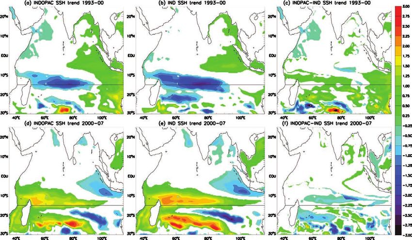
and its interpretation,” we review the observations        continental heating during boreal summer leads to a
     and current understanding of Indian Ocean decadal          strong meridional pressure gradient that drives the
     variability, delineating the effects of external forcing   southwest monsoon. The intense monsoon winds
     and internal climate variability whenever possible. In     induce a strong northward Somali Current and
     the final section, we briefly summarize the present        coastal upwelling near the coasts of Somalia and
     state of our knowledge and list major issues that need     Oman (Figs. 2b,d). During the winter monsoon,
     to be resolved.                                            surface winds (Fig. 2a) and ocean circulation (Fig. 2c)
                                                                reverse direction across the entire basin north of
     INDIAN OCEAN CIRCUL ATION AND                              10°S. By contrast, south of 10°S the South Equatorial
     INTERANNUAL CLIMATE VARIATIONS.                            Current (SEC) flows westward all year long under
     Here, we introduce the most important concepts that        the influence of relatively steady trade wind forcing.
     are essential for discussing decadal Indian Ocean             Warm water with SSTs > 28°C (the so-called warm
     variability. A detailed review of Indian Ocean circu-      pool) occupies a large portion of the tropical Indian
     lation and climate variability can be found in Schott      Ocean north of 10°S, with cooler temperatures to the
     and McCreary (2001) and Schott et al. (2009).              south and in the upwelling zones off Oman and the
                                                                Horn of Africa (Figs. 2a,b). The north Indian Ocean
     Indian Ocean circulation. In contrast to the Pacific       gains heat on an annual average via air–sea fluxes and
     and Atlantic Oceans, the Indian Ocean is bounded           this heat gain is transported across the equator to the
     to the north by the Asian landmass. As a result, the       south within the wind-driven cross-equatorial cell

Fig. 2. (a) January and (b) July monthly SST climatology (color) and surface wind stress (arrows) from HadISST
(Rayner et al. 2006) and ECMWF operational analysis/reanalysis winds (Balmaseda et al. 2008) for the 1960–
2009 period; (c) January and (d) July depth of 20°C isotherm (D20; color) averaged for 2001–12 period based
on in situ temperature data (Hosoda et al. 2008) and surface currents from Ocean Surface Current Analyses
Real-Time (OSCAR) data (arrows; Bonjean and Lagerloef 2002) averaged for 1992–2012. Large bulk arrows
identify the Leeuwin Current, Agulhas Current, ITF, SEC, and Somali Currents. The black boxes show the
thermocline ridge region.

1682 |      NOVEMBER 2014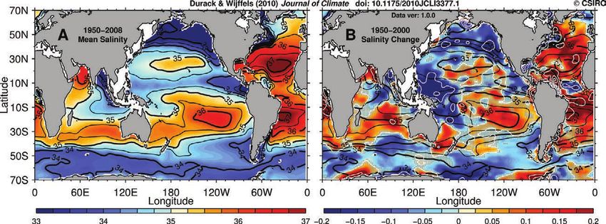
(CEC; Fig. 3). The surface branch of the CEC flows
southward across the equator, while the subsurface
branch is associated with cold thermocline water
that flows northward within the Somali Current,
upwelling near the coasts of Somali and Oman
(Miyama et al. 2003; Lee 2004; Schott et al. 2004).
   Unlike the prevailing easterly trades in the equato-
rial Pacific and Atlantic, annual-mean surface winds
in the equatorial Indian Ocean are westerlies. In the
tropical south Indian Ocean, wind stress curl asso-
ciated with easterly trade winds south of ~10°S and
the westerly winds farther north induce open-ocean
upwelling in the western basin between 12° and 2°S
(McCreary et al. 1993; Murtugudde and Busalacchi
                                                             F ig . 3. Schematic diagram showing the zonal- and
1999). This upwelling causes the thermocline shoal
                                                             time-mean meridional overturning circulation of the
in this latitude band, which is thus referred to as the      upper Indian Ocean that consists of a STC and CEC.
thermocline ridge region (Hermes and Reason 2008;            Adapted from Lee (2004).
Yokoi et al. 2008, 2009; boxed areas of Figs. 2c,d).
The existence of this upwelling induces a secondary          IOD is associated with a cold SST anomaly (SSTA)
overturning circulation referred to as the subtropical       in the eastern tropical Indian Ocean and warm
cell (STC; Miyama et al. 2003; Lee 2004; Schott et al.       SSTA in the western tropical basin (Fig. 4), reaching
2004; Fig. 3), which is fed in part by waters subducted      peak amplitudes during boreal fall (September–
(pumped down) into the thermocline in the south-             November). Like ENSO, the IOD is linked to warm
eastern Indian Ocean (e.g., Schott et al. 2009).             pool deep convection and the Indo-Pacific Walker
   The Indian Ocean is fed to the east by water              circulation. It has also been suggested that the IOD
coming from the western Pacific via the Indonesian           is an integral component of the tropical biennial
Throughflow (ITF). Part of the ITF feeds upwell-             oscillation (Loschnigg et al. 2003; Meehl et al. 2003).
ing in the thermocline ridge region of the STC and              Two other modes of interannual SST variability
some directly flows southward along the west coast           have also been identified: the Indian Ocean basin
of Australia in the Leeuwin Current. The major-              mode and the subtropical SST dipole. The basin mode
ity of the ITF, however, flows westward across the           features a basinwide warming (or cooling) pattern
Indian Ocean in the South Equatorial Current and             that primarily results from ENSO-induced changes
southward through the Mozambique Channel to the              in cloud cover and thus in shortwave radiation over
Agulhas Current where part of it enters the Atlantic         the Indian Ocean (Klein et al. 1999). It is maintained
near the southern tip of Africa (Figs. 2c,d). The rest       beyond the termination of ENSO events by Indian
returns eastward around 25°S, where it feeds into the        Ocean air–sea interactions and ocean dynamics (Du
Leeuwin Current (e.g., Reid 2003; McCreary et al.            et al. 2009). The subtropical SST dipole varies inter-
2007; Palastanga et al. 2007).                               annually with peak development in austral summer
                                                             (Behera and Yamagata 2001; Suzuki et al. 2004). A
Interannual climate variability. Until the late 1990s, the   positive phase is characterized by warm SSTA in the
scientific community focused most of its efforts on          southwestern Indian Ocean south of Madagascar and
the tropical Pacific, which hosts the powerful ENSO          cold SSTA in the eastern Indian Ocean off Australia.
phenomenon [see McPhaden et al. (2006) for an                The Antarctic Circumpolar Wave (e.g., White and
introduction to this phenomenon]. Prior to that, no          Peterson 1996) and air–sea interaction in the tropical
independent mode of interannual variability had been         Indo-Pacific basin may contribute to its generation
identified in the Indian Ocean. With the discovery           (Morioka et al. 2012, 2013).
of the Indian Ocean dipole (IOD; Saji et al. 1999;
Webster et al. 1999), however, it was realized that          OBSERVED DECADAL VARIABILITY AND
ocean–atmosphere interactions in the Indian Ocean            ITS INTERPRETATION. Warming trends and
can also give rise to significant climate fluctuations.      decadal variations. Long -term trends. Upper-ocean
Like ENSO, the IOD varies on interannual time                heat content reveals a warming trend of the Indian
scales, sustained through positive feedbacks between         Ocean since the 1950s (Levitus et al. 2009; Xue et al.
equatorial winds and zonal SST gradients. A positive         2012; Fig. 1). The Hadley Centre Sea Ice and Sea

AMERICAN METEOROLOGICAL SOCIETY                                                              NOVEMBER 2014         | 1683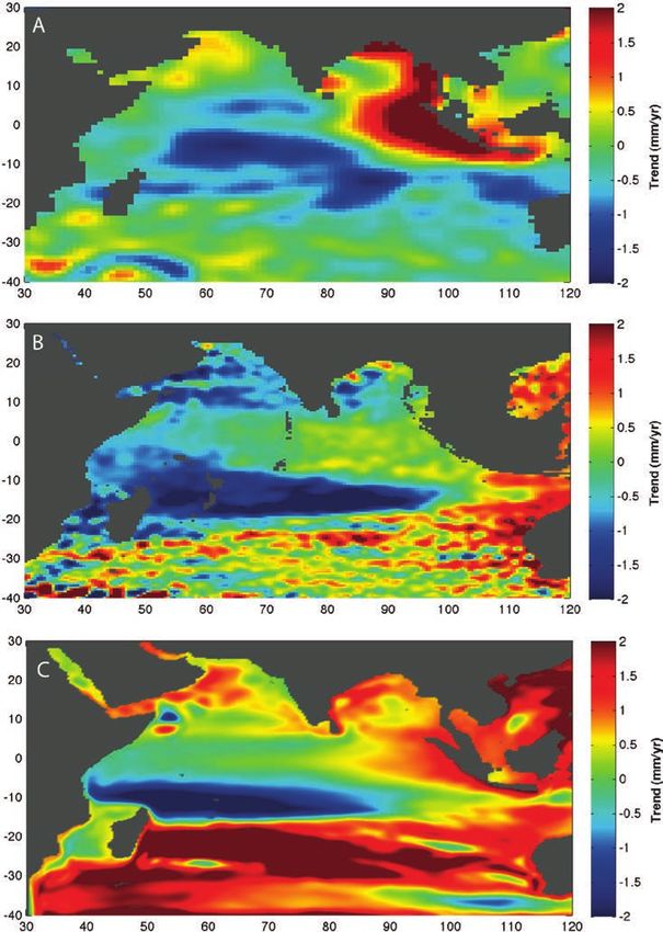
Fig. 4. (left) September, October, and November mean SSTA for the 1997 IOD event, based on the detrended
and demeaned SST from 1920 to 2011; (right) dipole mode index (DMI; black) for each year, which is defined
as the September, October, and November mean SSTA difference between the western pole (10°S–10°N,
50°–70°E) and eastern pole (10°S–0°, 90°–110°E); the red curve is 8-yr low-passed DMI, which shows decadal
variability. The red dashed vertical line marks the 1997 IOD.

     Surface Temperature dataset (HadISST; Rayner et al.      increasing Indian Ocean surface wind speed from
     2003) suggests that the tropical Indian Ocean has        1981 to 2005 (Yu and Weller 2007). This difference
     generally warmed faster than most regions of the         between models and observations may arise because
     tropical Pacific and Atlantic since the 1950s, with an   the models could not properly simulate Indian Ocean
     accelerated warming since the 1970s (Fig. 5; Hoerling    regional convection and the atmospheric circulation
     et al. 2012). In all SST datasets, the northern Indian   response to warming (Meng et al. 2012). Alternatively,
     Ocean has slower warming rates than the equatorial       the observed wind trend over the period 1981–2005
     zone, with warming signals that qualitatively agree      may reflect internal decadal variability that is sig-
     among different datasets. However, there are apparent    nificantly damped in the ensemble means of climate
     differences in the regional magnitudes and spatial       model solutions.
     structures of this warming, which underscore the            Attempts have also been made to explain the
     uncertainty in quantifying regional warming rates.       slower warming rate in the north Indian Ocean
        Climate model simulations with and without            (Figs. 1, 5). In this region, the effects of anthropogenic
     anthropogenic greenhouse gases demonstrate that          greenhouse warming are compensated by enhanced
     increases in these gases are the primary cause for       evaporative cooling and reduced solar radiation from
     the observed warming trends (e.g., Hansen et al.         South Asian aerosols (Chung and Ramanathan 2006).
     2002; Reichert et al. 2002; Gent and Danabasoglu         Despite the slow rate, the north Indian Ocean still
     2004; Gregory et al. 2004; Pierce et al. 2006; Hegerl    exhibits “warming.” This warming largely results
     et al. 2007; Gleckler et al. 2012). Attempts have been   from a spin down of the CEC since the 1950s and
     made by analyzing climate model simulations to           1960s (Schoenefeldt and Schott 2006; Trenary and
     understand the physical processes through which          Han 2008). A weaker CEC reduces the southward
     anthropogenic forcing causes the observed near-          transport of warm surface water from, and north-
     surface warming. Du and Xie (2008) argued that the       ward transport of cold thermocline water into, the
     steady warming of Indian Ocean SST since the 1950s       north Indian Ocean. In the south Indian Ocean,
     results from greenhouse gas–induced increases in         both increased surface heat flux and lateral advec-
     downward longwave radiation (see also Dong et al.        tion—likely from the Pacific Ocean—contribute to
     2014) amplified by the water vapor feedback and          the observed warming (Pierce et al. 2006). It is unclear
     from weakened winds that suppress turbulent heat         what the relative roles of anthropogenic forcing and
     loss from the ocean. Reduced upwelling may also          natural variability play in causing the CEC change.
     contribute to the surface warming over the ther-            Indian Ocean warming exhibits a complex
     mocline ridge region (defined in Fig. 2; Alory and       structure in the vertical: near-surface warming
     Meyers 2009). The weakened wind scenario proposed        accompanies upper-thermocline cooling in the
     by Du and Xie (2008) from model studies, however,        tropics and weaker warming beneath (Barnett
     appears to contradict the observed trend toward          et al. 2005; Pierce et al. 2006; Bindoff et al. 2007;

1684 |      NOVEMBER 2014
Fig. 5. (a) Linear trend of HadISST (Rayner et al. 2006) from 1950 to 2010; color (white) shading shows
values that are above (below) 95% significance; (b) – (d) As in (a), but for SST from Hurrell et al. (2008),
Kaplan et al. (1998), and Smith and Reynolds (2004) extended reconstructed (ER) data, respectively.
The two horizontal lines show 15°S and 15°N latitudes. The tropical Indian Ocean warms faster than
most regions of the tropical Pacific and Atlantic, except for a local area in the eastern Pacific south
of the equator. This trend pattern also holds for median Hadley Centre Sea Surface Temperature
dataset version 3 (HadSST3) data (Kennedy et al. 2011a,b) for the period of 1958–2006, even though
the warming rate over the Indo-Pacific warm pool is slower (not shown). HadSST3 data are available
until 2006 and have too many missing values in the tropical Pacific from 1950–57.

Fig. 6). This structure can only be reproduced when
anthropogenic greenhouse gases are included in
climate models (Barnett et al. 2005; Pierce et al.
2006). Han et al. (2006) and Trenary and Han (2008)
suggested that long-term changes in tropical Indian
Ocean winds are instrumental in causing the
thermocline cooling. The increasing southeasterly
trades strengthen the STC and the reduced wind
stress curl on the equator weakens the CEC (see also
Schoenefeldt and Schott 2006). These two effects
combine to induce heat divergence and thus cool
the upper thermocline over the thermocline ridge
region (Trenary and Han 2008). In contrast, Alory
et al. (2007) and Cai et al. (2008) suggested that in the
third phase of the Coupled Model Intercomparison
Project (CMIP3) climate models, the observed south
Indian Ocean thermocline cooling results mainly
                                                            Fig. 6. Linear trend of zonal-mean temperature across
from the shoaling thermocline in the western equato-
                                                            the Indian Ocean in the upper 1500 m from 1955 to 2003.
rial Pacific and wave transmission via the Indonesian       The contour interval is 0.05°C decade –1, and the dark
archipelago, driven by the relaxation of the easterly       solid lines are zero contours. Pink shading indicates val-
trades in the Pacific (McPhaden and Zhang 2002).            ues ≥ 0.025°C decade –1 and blue shading indicates values
In agreement with this hypothesis, analysis of              ≤ –0.025°C decade –1. Adapted from Bindoff et al. (2007).

AMERICAN METEOROLOGICAL SOCIETY                                                            NOVEMBER 2014         | 1685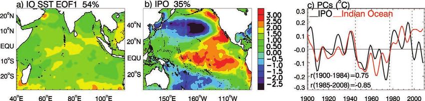
XBT data suggests a reduction of ITF transport by          et al. 2009; Hosoda et al. 2009; Durack and Wijffels
     ~2.5 Sverdrups (Sv; 1 Sv ≡ 106 m3 s–1) after 1976/77       2010; Helm et al. 2010). Regionally, SSS exhibits a
     (Wainwright et al. 2008). This analysis, however,          decreasing trend in the equatorial Indian Ocean, Bay
     was based on temperature data in the upper 700 m           of Bengal, and Southern Ocean, but an increasing
     only, without considering the effect of salinity and       trend in the subtropical south Indian Ocean and
     potential changes in transport below 700 m. Available      the Arabian Sea (Fig. 7). This spatial pattern of SSS
     multidecadal ocean data assimilation products do not       changes is consistent with the notion that saltier
     show evidence of a significant reduction of total (top     regions get saltier and fresher regions get fresher
     to bottom) ITF transport after 1976/77 as would be         under global warning. The surface freshening at
     required for a net ITF-mediated loss of mass from the      mid-to-high latitudes extends downward and equa-
     Indian Ocean basin (Lee et al. 2010). Schwarzkopf          torward to intermediate depths, primarily through
     and Böning (2011) demonstrated in controlled ocean         subduction and advection of salinity anomalies in
     general circulation model (OGCM) experiments the           the thermocline by the mean flow (Wong et al. 1999;
     role played by Indian Ocean winds in causing the           Bindoff and McDougall 2000; McDonagh et al. 2005;
     complex, zonal-mean vertical temperature structure         Bindoff et al. 2007; Böning et al. 2008; Roemmich and
     from 1960 to 1999, even though they emphasized the         Gilson 2009; Durack and Wijffels 2010). Freshening
     ITF effects on the thermocline cooling. Their solu-        in the abyssal southeastern Indian Ocean has also
     tions indeed produced stronger ITF effects on the          been observed (Johnson et al. 2008).
     cooling thermocline than that of Han et al. (2010).           Climate model simulations with and without
     The causes for these differences are discussed further     anthropogenic greenhouse gas forcing demonstrate
     in the “sea level variability” section.                    that observed salinity changes cannot be explained
                                                                by natural variability, either internal to the climate
     Decadal variations. Superimposed on these multi-           system or from external forcing via variations in
     decadal trends, near-surface temperature and upper-        solar output and volcanic eruptions (Durack et al.
     ocean heat content exhibit large-amplitude decadal         2012; Terray et al. 2012; Pierce et al. 2012). The ob-
     variations. Trenary and Han (2013) performed a             served changes, however, are consistent with the
     hierarchy of OGCM experiments and showed that the          changes expected due to the greenhouse gas–induced
     observed complex vertical structures of zonal-mean         warming and the resultant amplification of the global
     temperature vary from decade to decade, with strong        hydrological cycle (Held and Soden 2006).
     temperature variations generally occurring in the
     thermocline layer. Wind stress forcing over the Indian     Decadal variations. In addition to the multidecadal
     Ocean was primarily responsible for these variations,      trend since 1950 (Fig. 7), hydrographic data reveal
     but the ITF made significant contributions after           decadal fluctuations in salinity. Freshening in the
     1990. Near the surface, observations show significant      thermocline along 32°S before 1987 (Bindoff and
     decadal variations in basin-averaged upper-ocean           McDougall 2000) is consistent with global warming
     heat content (Fig. 1). The century-long coral-based        (Joos et al. 2003). However, between 1987 and 2002,
     records in the southwest Indian Ocean show large-          the trend reversed in the upper thermocline across
     amplitude decadal variability of SST, which is appar-      the entire 32°S section, accompanied by an increased
     ently associated with the natural decadal variability      oxygen concentration (McDonagh et al. 2005). This
     of ENSO (Cole et al. 2000; Cobb et al. 2001; Allan         signal appears to be associated with the natural
     et al. 2003; Zinke et al. 2004). Domingues et al. (2008)   decadal spinup of the south Indian Ocean subtropi-
     showed that volcanic eruptions induce significant          cal gyre over that period, as evident from enhanced
     decadal variability in global-mean temperature and         northward volume transport across 32°S (Palmer
     sea level (also see Zanchettin et al. 2012), but they      et al. 2004).
     did not examine volcanic effects separately for the           Variations in freshwater and heat transports in the
     Indian Ocean.                                              southern Indian Ocean are tied to the variability in
                                                                Agulhas Current transport (Bryden and Beal 2001),
     Salinity variability. Long -term trends . Recent obser-    whose leakage to the Atlantic has increased during
     vational studies indicate that globally, sea surface       the past few decades as suggested by satellite observa-
     salinity (SSS) has increased over the past few decades     tions (Rouault et al. 2009) and modeling studies [see
     in regions where evaporation exceeds precipitation         Beal et al. (2011) for a review]. The increased leakage,
     and decreased in regions of excess precipitation           however, is not supported by a recent analysis using
     (e.g., Roemmich and Gilson 2009; von Schuckmann            along-track satellite altimeter data (Le Bars et al.

1686 |      NOVEMBER 2014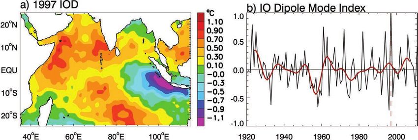
Fig. 7. (a) The 1950–2000 climatological-mean surface salinity. Contours every 0.5 on the practical salinity
scale (PSS) are plotted in black. (b) The 50-yr linear surface salinity trend [PSS (50 yr) –1]. Contours every 0.2
are plotted in white. Regions where the resolved linear trend is not significant at the 99% confidence level are
stippled in gray. Adapted from Durack and Wijffels (2010).

    2014). Thus, there remain uncertainties in detecting        et al. (2010) showed a distinct spatial pattern to the
    decadal variability in southern Indian Ocean fresh-         sea level trend since the 1960s, with sea level falling
    water and heat fluxes as well as their transports into      in the southwest tropical Indian Ocean and rising
    the Atlantic Ocean.                                         elsewhere. Similar patterns, evident in the thermo-
                                                                steric (i.e., temperature related) sea level derived from
    Sea level variability. Tide gauge observations. Sea level   in situ observations for the upper 700 m (National
    rise has been detected by tide gauge observations at        Research Council 2012) and in reconstructed sea
    various locations along coasts bordering the Indian         level data (Fig. 8) are well simulated by several ocean
    Ocean. In the northern Indian Ocean, sea level from         models (e.g., Timmermann et al. 2010; Schwarzkopf
    tide gauge records longer than 40 yr yield average          and Böning 2011; Dunne et al. 2012). The sea level fall
    sea level rise rates of 1.06–1.75 mm yr–1 over the          in the southwest tropical Indian Ocean also agrees
    1878–2004 period (Unnikrishnan and Shankar 2007).           with the observed subsurface cooling associated
    Overlying these trends, there is significant decadal        with the shoaling thermocline in the same latitudinal
    variability. At Mumbai, the century-long record             band (Fig. 6).
    shows that decadal variations in sea level mimic that          Han et al. (2010) suggested that the sea level trend
    of rainfall over the Indian subcontinent, indicating        from 1961 to 2001 is primarily driven by changing
    the effect of salinity on sea level variability when        surface winds associated with enhanced regional
    freshwater from monsoon rainfall f lows into the            Walker and Hadley circulations (also see Yu and
    Indian Ocean (Shankar and Shetye 1999). This sea            Zwiers 2010). On the other hand, Schwarzkopf and
    level/monsoon rainfall correlation may also reflect         Böning (2011) suggested a considerably larger ITF
    the effects of monsoon winds on sea level, which com-       influence. The divergence between these two studies,
    bine with freshwater input from monsoon rainfall and        based primarily on model results, is probably due to
    river discharge to force a large sea level response at      the wind products that were used to force the ocean
    Mumbai. Along the west coast of Australia, tide gauge       models. Han et al. (2010) used 40-yr European Centre
    and satellite altimeter data reveal large-amplitude         for Medium-Range Weather Forecasts (ECMWF)
    decadal variability in sea level and in the Leeuwin         Re-Analysis (ERA-40) winds that do not show an
    Current, which are heavily influenced by decadal            apparent reduction in easterly trades in the equa-
    variability in the western tropical Pacific via the ITF     torial Pacific after 1977, while Schwarzkopf and
    (e.g., Lee 2004; Lee and McPhaden 2008; Feng et al.         Böning (2011) used National Centers for Environ-
    2004, 2010, 2011).                                          mental Prediction–National Center for Atmospheric
                                                                Research (NCEP–NCAR) reanalysis winds that show
    S ea level trend patterns . The sea level trend and         an evident reduction of Pacific easterly trades near
    decadal variability along Indian Ocean coasts are in        1977 (e.g., Feng et al. 2011). These results stress the
    part associated with basinwide sea level patterns. Han      importance of long-term changes in the Indo-Pacific

    AMERICAN METEOROLOGICAL SOCIETY                                                              NOVEMBER 2014          | 1687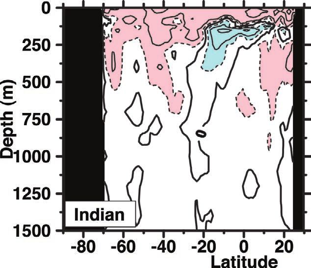
atmospheric circulation for describing and under-       changes in Indo-Pacific trade winds. Collectively,
     standing decadal changes in the Indian Ocean;           these wind and SSH changes imply opposite trends
     however, inconsistencies between different wind         in the transports of the Pacific and Indian Ocean
     products, ocean reanalysis datasets, and the lack of    STCs (see also Zhuang et al. 2013). Lee and McPhaden
     reliable observations prior to the 1980s before the     (2008) suggested that the decadal changes in the
     satellite era may cause significant uncertainties in    Pacific and Indian Ocean STCs during this period
     detecting atmospheric circulation changes (see the      were linked via the atmosphere through the Walker
     side bar for Indo-Pacific Walker circulation change)    circulation and via the ocean through the ITF.
     and in quantifying their impacts on Indian Ocean           To understand the causes for Indian Ocean
     sea level changes.                                      decadal sea level variability, Trenary and Han (2013)
                                                             and Nidheesh et al. (2013) performed a hierarchy of
      D ecadal sea level variations . Basinwide sea level OGCM experiments. The satellite observed basin-
      trend patterns also exhibit decadal variations. Lee wide SSH trend reversal from 1993–2000 to 2000–07
      and McPhaden (2008) detected in satellite observa- (Fig. 9) described in Lee and McPhaden (2008) was
      tions substantial decadal reversals in basinwide sea successfully simulated by the OGCMs (Figs. 10a,d).
      surface height (SSH) trends in the Indo-Pacific region This pattern reversal resulted primarily from Indian
      from 1993–2000 to 2000–06 associated with decadal Ocean wind forcing (Figs. 10b,e), with the effect of
                                                                        Pacific forcing transmitted through the
                                                                        Indonesian archipelago via the ITF contrib-
                                                                        uting most significantly in the eastern basin
                                                                        (Figs. 10c,f). Nidheesh et al. (2013) showed
                                                                        that thermal variations dominate the
                                                                        decadal sea level variability, with sizeable
                                                                        salinity contributions in only a few regions.
                                                                        The large-amplitude decadal variations in
                                                                        sea level in the southwest Indian Ocean
                                                                        thermocline ridge region were primarily
                                                                        caused by local Ekman pumping velocity
                                                                        associated with wind stress curl and by
                                                                        westward-propagating Rossby waves gen-
                                                                        erated by winds in the central and eastern
                                                                        basin (Trenary and Han 2013).
                                                                            Since the early 1990s, however, the
                                                                        ITF has increased its contribution in the
                                                                        thermocline ridge region and along the
                                                                        west coast of Australia (Trenary and Han
                                                                        2013). This increased Pacific influence is
                                                                        consistent with the decadal intensifica-
                                                                        tion of easterly trades and sea level in the
                                                                        western tropical Pacific (Merrifield 2011;
                                                                        Luo et al. 2012; Han et al. 2014), increased
                                                                        Makassar Strait transport (Susanto et al.
                                                                        2012), and enhanced ITF and Leeuwin
                                                                        Current transports (Feng et al. 2011) since
                                                                        the early 1990s. Enhanced transmission of
                                                                        ENSO signals at thermocline depth into
                                                                        the Indian Ocean since 1980 has also been
                                                                        suggested (Shi et al. 2007). Trenary and
                                                                        Han (2013) also found that in the subtrop-
F ig . 8. Regional sea level trends for 1961–2001 computed
from (a) the Church et al. (2004) reconstructed data, (b) the
                                                                        ics between 20° and 30°S, oceanic internal
Hamlington et al. (2011) reconstructed data, and (c) a Hybrid           variability makes significant contributions
Coordinate Ocean Model (HYCOM) simulation. Adapted from                 to the decadal variability of sea level and
Hamlington et al. (2011).                                               thermocline depth.

1688 |      NOVEMBER 2014
Fig. 9. (a) Linear trend of SSH anomaly (SSHA) from multisatellite merged French Archiving, Validation, and
Interpretation of Satellite Oceanographic (AVISO) data (Ducet et al. 2000) for the 1993–2000 period; values
exceeding 95% significance are shown; (b) As in (a), but for 2000–07. Units are centimeters per year. The hori-
zontal line marks the latitude of 15°S.
Fig. 10. Linear trends in SSHA for the period 1993–2000 for (a) HYCOM experiment with full forcing in both
the Indian and Pacific Oceans (referred to as INDOPAC), (b) HYCOM experiment with variability of the Pacific
forcing excluded (referred to as IND), and (c) DIFF = (INDOPAC – IND), which assesses the effect of Pacific
forcing via the Indonesian Archipelago and also includes oceanic internal variability effect; (d) – (f) As in (a) – (c),
but for the period of 2000–07. Values exceeding 95% significance are shown. Units are centimeters per year.
Adapted from Trenary and Han (2013).
Finally, Nidheesh et al. (2013) and Lee and variability over the Indian Ocean (Fig. 11). This
McPhaden (2008) are in basic agreement about the behavior is different from that on interannual time
role of atmospheric teleconnections between the scales, when basin-scale winds and SSH associated
Pacific and southwestern Indian Ocean over the last with ENSO and IOD significantly covary. These
20 yr. These teleconnections, however, break down conflicting results need to be reconciled, which may
when considering the longer 1966–2007 period, involve consideration of the possible varying rela-
during which large-amplitude decadal variations in tionship between the Pacific and Indian Oceans in
Pacific SSH and winds do not correspond to large different decades and the reliability of atmospheric
AMERICAN METEOROLOGICAL SOCIETY NOVEMBER 2014 | 1689reanalysis products in representing decadal variabil- trends (Cai et al. 2013). Zheng et al. (2010) examined
ity, especially before the satellite era. the impact of greenhouse warming on IOD behavior
[see Cai et al. (2013) for a review] and concluded that
Decadal modulation of interannual variability. Abram the increasing occurrence of positive IOD events in
et al. (2008) analyzed coral oxygen isotope records the past few decades results from a gradual increase in
and showed an increasing trend in the frequency and the mean west-minus-east SST gradient in the tropical
strength of IOD events during the twentieth century. Indian Ocean. As a result, the IOD index crosses the
Analyses of historical SST datasets and ocean reanaly- defined threshold more frequently near the end of the
sis products suggest that prior to 1920, negative IOD twentieth century. Climate model projections suggest
events dominated, whereas after 1950, positive IOD that under greenhouse gas warming, the frequency of
events prevailed (e.g., Kripalani and Kumar 2004; positive IOD events will increase by a factor of three
Ihara et al. 2008; Yuan et al. 2008; Cai et al. 2009). The near the end of the 21st century (Cai et al. 2014).
upward trend of the IOD index (see Fig. 4b) in recent Overlying this trend, there are decadal fluctuations
decades, however, appears in some SST datasets but in the IOD index (e.g., Ashok et al. 2004; Ihara et al.
not in others, highlighting the uncertainties in these 2008; red curve of Fig. 4; Figs. 12c,d,g,h) and decadal
Fig. 11. The first two EOF patterns of steric sea level anomalies over the (left) Indo-Pacific sector and (right)
their corresponding normalized PCs at decadal (7-yr low-passed) time scales from an OGCM experiment.
Arrows are the wind stress components regressed onto each normalized PC. The percentage explained by
each EOF is shown in parentheses. Adapted from Nidheesh et al. (2013).
1690 | NOVEMBER 2014Fig. 12. (a),(c) PCs and (b),(d) spatial amplitudes of the first and second EOF modes of the simulated decadal (9–35-yr bandpass) SSTA by a global coupled model control run. (e) – (h) As in (a) – (d), but for the observed decadal (9–35-yr bandpass) SSTA from extended reconstructed data of Smith and Reynolds (2004). Contour interval is 0.01°C and negative anomalies are shaded for the spatial amplitude (from Tozuka et al. 2007). AMERICAN METEOROLOGICAL SOCIETY NOVEMBER 2014 | 1691
changes in the Indian Ocean SST–ENSO (Annamalai            over the northwest Pacific (Xie et al. 2010; Chowdary
     et al. 2005) and IOD–ENSO–monsoon relationship             et al. 2012). The Indian Ocean subtropical dipole
     before and after 1976/77 (e.g., Allan et al. 2003; Clark   (“interannual climate variability” section) also
     et al. 2003; Meehl and Arblaster 2011, 2012). Decadal      undergoes decadal variations. In particular, its
     fluctuations of IOD index are not well correlated with     amplitude weakened but its correlation with ENSO
     decadal variations in the Niño-3 index—the SSTA            was enhanced after 1979/80 (Yan et al. 2013). The
     averaged over 5°S–5°N and 90°–150°W in the Pacific         reasons for this decadal variability in the subtropical
     and an indicator of ENSO variability (Ashok et al.         dipole are not clear.
     2004; Song et al. 2007; Tozuka et al. 2007). They are,
     however, highly correlated with Indian Ocean ther-         Decadal variability generated by processes internal to
     mocline depth and equatorial zonal wind anomalies          the Indian Ocean. On decadal time scales, a basinwide
     (Ashok et al. 2004), suggesting that ocean dynamics        warming/cooling pattern dominates Indian Ocean
     are involved. Since the time for low-latitude Rossby       SSTAs and explains 54% variance using HadISST
     waves to cross the tropical Indian Ocean is too short      (Fig. 13a). We dub this f luctuation the “decadal
     to account for decadal time scale variability, Tozuka      Indian Ocean basin mode” by analogy with the
     et al. (2007) concluded that decadal variations in the     basin mode that is evident on interannual time
     IOD are due to the skewness (asymmetry) of positive        scales. While this basin mode is positively corre-
     and negative IOD events.                                   lated with the IPO before 1985, analogous to ENSO
         Meehl and Arblaster (2011, 2012) suggested that        impact on the interannual Indian Ocean basin mode
     interdecadal Pacific oscillation (IPO; Power et al.        (“interannual climate variability” section), the corre-
     1999; Fig. 13) can significantly modulate the relation-    lation reverses to negative after 1985 (Fig. 13c). Causes
     ship between the Asian–Australian monsoon, ENSO,           for this change in character remain unclear. It may
     and IOD. Given that the IPO index—the principle            indicate that the Indian Ocean plays an increasingly
     component (PC) of the leading empirical orthogonal         important role in shaping Indo-Pacific decadal cli-
     function (EOF) of Pacific decadal SSTA—is highly           mate under global warming (Han et al. 2014) or that
     correlated with ENSO indices (Han et al. 2014), the        it is due to natural variability (forced or internally
     low IOD–ENSO correlation on decadal time scales            generated) in the climate system.
     discussed above requires an explanation. It is possible        To understand the effect of air–sea interaction in
     that the IOD possesses a component independent of          the Indian Ocean in generating decadal variability,
     IPO, even though IPO can modulate its variability.         Allan et al. (1995) and Reason and Lutjeharms (2000)
         In addition to the IOD, the Indian Ocean basin         analyzed detrended observational datasets and identi-
     mode (“interannual climate variability” section)           fied decadal variations in SST, sea level pressure (SLP)
     shows pronounced interdecadal modulation in its            and surface winds during austral summer and for
     variance and correlation with ENSO, strengthening          the annual mean for four epochs: 1900–20, 1921–41,
     when ENSO variance is high and weakening when it           1942–62, and 1963–83 (also see Jones and Allan 1998;
     is low (Chowdary et al. 2012). This decadal modula-        Reason et al. 1998). The first two epochs showed rela-
     tion has large impacts on atmospheric variability          tively weak south Indian Ocean SLP and anticyclonic

Fig. 13. (a) The leading EOF of SST for the Indian Ocean, based on 8-yr low-pass filtered monthly HadISST
from 1900 to 2008, which explains 54% variance. The monthly SST data from 1870 to 2012 are first detrended
and demeaned and then the Lanczos low-pass filter with half power point placed at 8-yr period is applied. The
filtered SST from 1900 to 2008 is chosen to perform the EOF analysis. (b) As in (a), but for the Pacific SST,
which represents the IPO spatial pattern and explains 35% variance. (c) The leading PC (PC1) of 8-yr low-passed
SST for the Pacific (black curve) and Indian Ocean (red). Adapted from Han et al. (2014).

1692 |      NOVEMBER 2014
surface winds, which were associated with cold SSTAs interaction play in generating Indian Ocean decadal
across the midlatitudes (south of 30°S) and weaker, SSTAs? What are the effects in the Indian Ocean of
warm SSTAs in the subtropical south Indian Ocean. stochastic atmospheric forcing, which has been shown
The last epoch shows a significant intensification of to be important for generating Pacific decadal vari-
the anticyclone, which was associated with warm ability? What is the relative importance of external
SSTAs in the midlatitudes and weaker, cold SSTAs forcing (greenhouse gases, aerosols, solar forcing,
in the tropics. During 1942–62 (the third epoch), and volcanoes) versus natural internal variability in
the atmospheric circulation underwent a transition generating decadal Indian Ocean variability? These
between the first two epochs and the last. are important unanswered questions.
Standalone OGCM experiments show that the ob-
served decadal SSTA pattern in the southern Indian SUMMARY, ISSUES, AND CHALLENGES.
Ocean is well reproduced by the Indian Ocean surface In situ and satellite observations, ocean–atmosphere
forcing primarily through surface heat fluxes (Reason reanalysis products, and reconstructed datasets show
2000). By contrast, when forced by idealized SSTAs multidecadal trends in upper Indian Ocean heat
prescribed in the southern Indian Ocean where the content, temperature, salinity, and sea level since
observed SSTAs are large in amplitude, the AGCM the 1950s. Model experiments suggest that all the
could not reproduce the observed winds and SLP observed trends are associated with anthropogenic
(Reason and Lutjeharms 2000). The authors con- forcing to some degree. While basinwide warming
cluded that the decadal SSTAs in the southern Indian is attributed to forcing by anthropogenic greenhouse
Ocean might be forced by a global atmospheric mode, gases, the slower warming rate over the north Indian
with Indian Ocean air–sea interaction providing Ocean results from reduced solar radiation caused by
some regional feedback. The caveat for this experi- the loading of the atmosphere with anthropogenic
ment was that the SSTAs were prescribed only in the aerosols of South Asian origin. The basin-scale near-
midlatitudes of the southern Indian Ocean. SSTAs surface warming accompanies thermocline cooling
have smaller amplitudes in the equatorial and north- and falling sea level over the tropical–subtropical
ern Indian Ocean basins, but their effects on convec- south Indian Ocean. The distinct spatial structures of
tion can be large there because they are superimposed temperature and sea level can largely be explained by
on high mean SSTs (Fig. 2). Given the nonlinear the changing wind patterns, which are partly driven
dependence of convection on SST, tropical variability by the Indo-Pacific warming. On the other hand,
can affect the extratropics via atmospheric telecon- there is no consensus on the contribution to these
nections, an issue that was not explored in Reason and trends from the Pacific via the ITF. The SSS trend
Lutjeharms (2000). Krishnamurthy and Goswami has a spatial pattern resembling that of the mean SSS,
(2000) analyzed the NCEP–NCAR reanalysis and which is consistent with an enhanced hydrological
suggested that SST and SLP patterns over the Indian cycle associated with global warming. There is an
Ocean, Pacific, and Atlantic regressed onto an 11-yr apparent upward trend of positive IOD occurrence
running-mean Indian summer monsoon rainfall since the 1950s, which is attributed to the mean state
index that resembles those regressed onto an 11-yr change associated with global warming.
running-mean Niño-3 index. They argued that these It is important to understand decadal changes
results support a hypothesis that decadal variations of the Indo-Pacific winds and Walker circulation
of the Indian summer monsoon and tropical SST are because they largely drive the spatial structures of
parts of a tropical coupled ocean–atmosphere mode Indian Ocean sea level and thermocline changes.
that is connected by the Walker and Hadley circula- There is, however, no consensus on trends in equato-
tions (also see Meehl et al. 1998). rial Indian Ocean westerly winds and the Indo-Pacific
Trenary and Han (2013) showed that variability Walker circulation over the past 50–100 yr. Some
internal to the Indian Ocean can generate decadal observational analyses indicate that Indo-Pacific
SST variations in the southern Indian Ocean. Walker circulation is weakening while others indicate
Similarly, Compo and Sardeshmukh (2010) showed it is strengthening. AGCMs forced by different SST
that the Indian Ocean SST trend pattern from 1949 products produce divergent results. Hence, further
to 2006 is dominated by variability unrelated to research is needed to resolve these issues.
ENSO. In addition, they found that for 1871–2006, Superimposed on these long-term trends are
Indian Ocean SST variability related to ENSO and decadal time scale fluctuations. The observed decadal
that not related to ENSO have comparable ampli- variability in the Indian Ocean basinwide sea level,
tudes. Just what role does the Indian Ocean air–sea salinity, and thermal structure results primarily from
AMERICAN METEOROLOGICAL SOCIETY NOVEMBER 2014 | 1693forcing by Indian Ocean winds, with a significant into account both forced climate change and natural
contribution from the ITF in the interior of the south decadal-scale climate variability. Most of these efforts
Indian Ocean after 1990. Near the coasts, salinity vari- have adopted a global perspective, but with emphasis
ability due to the river discharge may also contribute on variations in the Atlantic and Pacific. There are
to decadal sea level fluctuations. Decadal modulation recent studies showing predictive skill in the Indian
of the interannual Indian Ocean basin mode, the IOD, Ocean at interannual time scales, such as for the 2006
and subtropical dipole are observed. While decadal and 2007 IOD (Luo et al. 2008); also there is evidence
variability of the interannual basin mode is tied to of predictive skill for Indian Ocean SST at 2–9-yr lead
decadal variability in ENSO, decadal modulations of times, which is attributed to variations in radiative
the subtropical dipole and IOD are not well under- forcing, volcanic aerosols, and the long-term warming
stood. Some studies suggest that decadal fluctuations trend (Corti et al. 2012; Guemas et al. 2013). The pre-
of the IOD are not correlated with the decadal vari- dictive skill for Indian Ocean SST on 10-30-yr time
ability of ENSO or the IPO, while some climate model scales and the effect of Indian Ocean SST variability
studies suggest that the IPO can modulate the IOD via on regional and global decadal climate prediction,
changes in the Walker circulation. Thus, the relative however, remain largely unexplored.
importance of variability internal to the Indian Ocean From an oceanographic perspective, the generation
versus Pacific forcing of the IOD at decadal time scales of decadal time scale variability in the Indian Ocean
remains an open question. involves processes operating both at and below the
Basinwide patterns of decadal covariability in SST, air–sea interface. Subsurface oceanic processes in
SLP, and surface winds have been detected for the particular provide the memory of the system because
past century. Data analyses, together with dynamical of the vast thermal inertia of the interior ocean.
model experiments, suggest that the observed decadal Development of successful decadal prediction schemes
variability in Indian Ocean SST results from atmo- will rely critically on our understanding of the origins
spheric forcing associated with global-scale variations and mechanisms of Indian Ocean decadal variability.
in circulation, with Indian Ocean SST providing Advancing our understanding of that variability will
only a weak local feedback to the atmosphere. Recent require reliable, long-term surface and subsurface
studies show that large-amplitude decadal SST vari- oceanic observations. Continuous progress is being
ability over the Indian Ocean unrelated to ENSO is made to quality control existing historical datasets
comparable in magnitude to that which is related to for climate research applications (e.g., Gouretski
ENSO. The dominant pattern of decadal SST vari- and Koltermann 2007; Wijffels et al. 2008; Ishii and
ability, which we dub the decadal Indian Ocean Kimoto 2009; Levitus et al. 2009; Willis et al. 2009;
basin mode, also appears to be partially independent Gouretski and Reseghetti 2010), but there remains
from the IPO and to have impacts on tropical Pacific an imperative for sustained in situ and satellite ob-
variability particularly since the mid-1980s. What servations into the future as well. Recent advances
are the processes internal to the Indian Ocean in in observing system development, most notably with
generating the observed decadal variability? Ocean the implementation of the Indian Ocean Observing
modeling results suggest that oceanic instabilities System (IndOOS), have significantly enhanced our
contribute to decadal SST variability in the extratropi- capability to conduct Indian Ocean research. IndOOS
cal south Indian Ocean. While the role of stochastic includes the Research Moored Array for African–
atmospheric forcing in generating decadal variabil- Asian–Australian Monsoon Analysis and Prediction
ity has been investigated in detail in the Pacific and (McPhaden et al. 2009); the Argo network (www.argo
Atlantic Oceans, it has not been carefully studied for .ucsd.edu); and other elements designed to comple-
the Indian Ocean. What are the effects of stochastic ment satellite observations of wind stress, SST, sea
forcing and oceanic Rossby waves in causing Indian level, and gravity. Collectively, these satellite and in
Ocean decadal variability, and what is the relative situ measurements systems are providing indispens-
importance of forcing that is external to the Indian able observational resources for studies of decadal
Ocean (natural and anthropogenic forcing plus the variability and predictability in the Indian Ocean
influence of ENSO) versus processes internal to the region. Recent advances in salinity remote sensing
Indian Ocean in generating Indian Ocean decadal from Soil Moisture Ocean Salinity (SMOS; www.esa
variability? These are outstanding questions that need .int/Our_Activities/Observing_the_Earth/SMOS)
to be addressed. and Aquarius/Satelite de Aplicaciones Cientificas-D
Efforts to predict the evolution of climate over (SAC-D; http://aquarius.nasa.gov) missions are
the next several decades have recently begun, taking broadening the frontiers of the Indian Ocean research
1694 | NOVEMBER 2014You can also read