Genetic mapping on local Swedish chicken breeds

Genetic mapping on local Swedish
 chicken breeds

 Samrawit Tsehay Gebeyehu

Independent project: 30 hp
Swedish University of Agricultural Sciences, SLU
Faculty of Veterinary Medicine and Animal Science
Department of Animals Breeding and Genetics
European Master in Animal Breeding and Genetics (EMABG)
Uppsala 2021

Genetic mapping on local Swedish chicken breeds

Samrawit Tsehay Gebeyehu

Supervisor: Dr. Anna Maria Johansson, SLU, Department of Animal
 Breeding and Genetics
Supervisor: Prof. Dr. Henner Simianer, UGOE, Department of Animal
 Science
Examiner: Dr. Martin Johnsson, SLU, Department of Animal Breeding and
 Genetics

Credits: 30 hp
Level: Advanced, A2E
Course title: Independent project in Animal Science
Course code: EX0870
Programme/education: European Master in Animal Breeding and Genetics (EMABG)
Course coordinating dept: Department of Animals Breeding and Science

Place of publication: Uppsala
Year of publication: 2021

Keywords: chicken, genetic diversity, GWAS, plumage color, SNP, Swedish
 chicken breed

Swedish University of Agricultural Sciences
Faculty of Veterinary Medicine and Animal Science
Department of Animals Breeding and Genetics

Publishing and archiving
Approved students’ theses at SLU are published electronically. As a student, you
have the copyright to your own work and need to approve the electronic
publishing. If you check the box for YES, the full text (pdf file) and metadata will
be visible and searchable online. If you check the box for NO, only the metadata
and the abstract will be visible and searchable online. Nevertheless, when the
document is uploaded it will still be archived as a digital file.
If you are more than one author you all need to agree on a decision. Read about
SLU’s publishing agreement here: https://www.slu.se/en/subweb/library/publish-
and-analyse/register-and-publish/agreement-for-publishing/.

☒ YES, I/we hereby give permission to publish the present thesis in accordance
with the SLU agreement regarding the transfer of the right to publish a work.

☐ NO, I/we do not give permission to publish the present work. The work will
still be archived and its metadata and abstract will be visible and searchable.

 i

Abstract
Today, genetic studies are gaining popularity around the world, especially in the developed world.
The study of genetic diversity is the basis for genetic protection and future breed improvement. The
current study aimed to assess the genetic diversity, genetic relationship, and to identify the genes
affecting the plumage colors of eight Swedish chicken breeds. There are about 11 breeds of Swedish
chickens in Sweden. The study breeds were Gotlandshöna, Öländsk dvärghöna, Kindahöna,
Hedemorahöna, Skånsk blommehöna, Åsbohöna, Ölandhöna, and svarthöna chicken.
A total of 83 chickens were genotyped using a 62K SNP chip. The mean observed heterozygosity
of the study breeds was 0.40 and the mean inbreeding coefficient (F) of the study breeds calculated
from the discrepancy of observed and expected heterozygotes was -0.07. The mean FST of the study
breeds was 0.36, which indicated that the Swedish chicken breeds were very diverse. The study
breeds formed 3 main clusters in the multi-dimensional scaling (MDS) plot based on their genetic
relationship, where most of the breeds were grouped in one of the main groups. Due to population
structure, it was not possible to identify potential SNPs involved in plumage color variation.
To do GWAS for plumage color variability of Swedish chickens, the sample size must be much
larger. The current study on genetic diversity may help to strengthen the genetic conservation
program, such as, eliminating inbreeding and conducting additional molecular-based studies.
Further research into plumage color variability should be done, by including many more individuals.

Keywords: chicken, genetic diversity, GWAS, plumage color, SNP, Swedish chicken breed

 ii

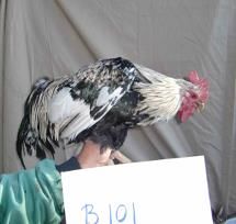
Table of Contents

List of tables ............................................................................................................................ v

List of figures .......................................................................................................................... vi

List of figures in appendix 1 .................................................................................................... vii

List of figures in appendix 2 ................................................................................................... viii

List of figures in appendix 3 ..................................................................................................... ix

List of abbreviations................................................................................................................. x

1. INTRODUCTION............................................................................................................... 1
 1.1. Background .................................................................................................................... 1
 1.2. Statement of Problem .................................................................................................... 3
 1.3. Objectives....................................................................................................................... 3

2. LITERATURE REVIEW ....................................................................................................... 4
 2.1. Genetic diversity within and between breeds ................................................................ 4
 2.2. Genetics of plumage color ............................................................................................. 6

3. MATERIAL AND METHODS .............................................................................................. 9
 3.1. Data source .................................................................................................................... 9
 3.2. Chicken Samples ............................................................................................................ 9
 3.3. DNA-Samples and Genotyping ..................................................................................... 10
 3.4. Phenotypic traits used in the study .............................................................................. 10
 3.5. SNP quality control for diversity analysis ..................................................................... 11
 3.6. Statistical analysis........................................................................................................ 11
 3.6.1. Diversity analysis ..................................................................................................... 11
 3.6.2. Genetic relationship ................................................................................................ 13
 3.7. Genome-wide association test ..................................................................................... 14

4. RESULT and DISCUSSION ............................................................................................... 16
 4.1. Genetic diversity within and between breeds .............................................................. 16
 4.2. Genetic relationship between breeds .......................................................................... 22
 4.3. GWAS for phenotypic traits ......................................................................................... 23

 iii

5. CONCLUSION ................................................................................................................ 26

References ............................................................................................................................. 27

Acknowledgments ................................................................................................................. 37

Appendix 1: GWAS for the entire body parts .......................................................................... 38

Appendix 2: GWAS for different body parts ............................................................................ 41

Appendix 3: Principal component analysis .............................................................................. 44

 iv

List of tables

Table 1. SNP quality control ............................................................................................................ 11
Table 2: The measure of genetic diversity for the study breeds .................................................... 20
Table 3. Pairwise FST estimate between breeds ............................................................................. 21

 v

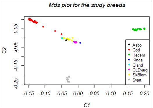
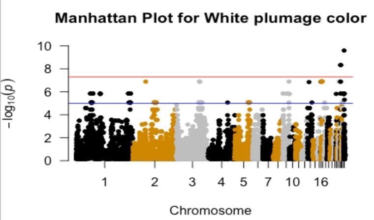
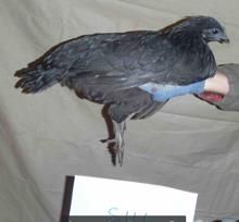
List of figures

Figure 1. Svart chicken with black plumage color (Left); SkBlom chicken with black-white blooming
plumage color (Right) ..................................................................................................................... 10
Figure 2. MDS plot of the study breeds; MDS plot indicated distance and similarity between
breeds, C1 is the largest component of variability, and C2 indicated the second-largest component
of variability .................................................................................................................................... 23
Figure 3. QQ plot for black wing color with inflation factor (=2.4265) ......................................... 24
Figure 4. QQ plot for Gotlands breed for light-brown plumage color using principal components 25
Figure 5. QQ plot for Gotlands breed for black-tail plumage color using principal components .... 25

 vi

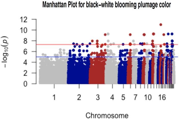
List of figures in appendix 1

Figure 1. Manhattan plot for white plumage color ........................................................................ 38
Figure 2. QQ plot for white plumage color with inflation factor (=2.41228) ................................ 38
Figure 3. Manhattan plot for black plumage color ......................................................................... 39
Figure 4. QQ plot for black plumage color with inflation factor(=2.70855).................................. 39
Figure 5. Manhattan plot for black-white blooming plumage color ............................................... 40
Figure 6. QQ plot for black-white blooming plumage color with inflation factor (=2.8643) ........ 40

 vii

List of figures in appendix 2

Figure 1. Manhattan plot for black-wing color ............................................................................... 41
Figure 2. Manhattan plot for brown-black neck color .................................................................... 41
Figure 3. QQ plot for brown-black neck color with inflation factor (=3.26639) ............................ 42
Figure 4. Manhattan plot for black-tail color.................................................................................. 42
Figure 5. QQ plot for black-tail color with inflation factor (=2.39234) ......................................... 43

 viii

List of figures in appendix 3

Figure 1. Bi-plot principal component (PCs) analysis for Gotlands breed ....................................... 44

 ix

List of abbreviations

Chr – Chromosome
F --- Inbreeding coefficient
FIS--- Individual heterozygosity relative to the subpopulation
FST – Fixation index
Geno ---Missing genotype rate
GWAS ---Genome-wide association study
HWE ---Hardy Weinberg Equilibrium
MAF ---Minor allele frequency
Mds ---Multi-dimensional scaling
Mind ---Missing genotype rate
Ne ---Effective population size
PCs --- principal components
PIC ---Polymorphism information content
QQ plot ---Quantile- Quantile plot
SNP ---Single nucleotide polymorphism
 ---genomic inflation factor

 x

1. INTRODUCTION

1.1. Background
The ancestor of the domestic chickens (Gallus gallus domesticus) originated from
the wild junglefowl (G. gallus) in Southeast Asia (Crawford, 1990; Moiseyeva et
al., 2002). The genus gallus had four main wild species, which are expected to be
the ancestor of domestic chickens; red junglefowl (G. gallus), gray junglefowl (G.
sonnerati), green junglefowl (G. varius), and Sri Lankan junglefowl (G. lafayetii).
However, the genetic predisposition of each species to the modern chicken has not
been well discovered (Dessie et al., 2012; Moiseyeva et al., 2002), but, based on
the archaeological and molecular evidence, it is widely described that the red
junglefowl is the main ancestorial origin of domestic chicken.

Local chicken breeds make a significant economic contribution in many countries
(Barua &Yoshimura, 2017; Kingori et al., 2010). They are highly adapted to the
local environmental condition and require a minimum input for farming (Kaya and
Yildiz, 2008). They are also selected by their nature and may have unique genetic
differences. However, they have poor performance and less attention to genetic
protection than other breeds (Blackburn, 2006; FAO, 2007). Most phenotypic and
genetic studies have also focused on high-performing commercial chicken breeds
(FAO, 2011; Granevitez et al., 2007).

The selection and breeding of some poultry began in the mid-19th century (FAO,
2007). The growing demand for improved breeds of chickens and the availability
of modern technologies are increasing (Englund et al., 2014). A long-term breeding
effort supports the improved breeds to dominate the current poultry production
sector. Indigenous breeds are threatened by the commercialization of improved
breeds. Poultry breeding supports the use of improved breeds and the replacement
of indigenous breeds with improved breeds (FAO, 2011; Granevitez et al., 2007).

There are about eleven local Swedish chicken breeds in Sweden (Abebe et al.,
2015). Before being rescued by the Swedish Local Chicken Association, the
number of individuals of the breeds was very small (Englund et al., 2014). The
association has maintained these chickens directly in the form of a gene bank in
collaboration with its members and other partners (http://www.kackel.se) (Abebe
et al., 2015). The individual chicken was originated from different areas of Sweden
and may have been selected for a variety of adaptations. Although they pass

 1

between a lot of bottle-neck, there are many phenotypic variabilities (Englund et
al., 2014).

Previous studies on the genetic diversity of local Swedish chicken have reported a
lower genetic diversity among breeds. A study on nine breeds using the mtDNA D-
loop reported a limited mtDNA diversity between breeds with seven different
haplotypes and most of the breeds had the same haplotype (Englund et al., 2014).
A limited genetic difference between Swedish chicken breeds was also reported by
Abebe and others (2015) using a 24K SNP chip. In all studies, relatively high
molecular co-ancestry has been found, which may increase the rate of inbreeding
in successive generations.

Recent advances in genetic markers provide many options for estimating genetic
diversity among populations at the DNA level, rather than identifying species based
on their phenotypic traits. Microsatellites are very numerous and are distributed
evenly throughout the genome at high levels of mutations (Anmarkrud et al., 2008).
they provide accurate information because they have a higher rate of occurrence of
common alleles and have more polymorphism over the population (Maudet et al.,
2002). Recently, a lot of researches have been done to assess the genetic diversity
of chickens using microsatellite markers, and the results are a clear indicator of the
usefulness of these markers for biodiversity research (Kaya & Yildiz, 2008;
Ramadan et al., 2012; Wilkinson et al., 2012).

In poultry, plumage color is an economically important trait and has cultural value
in many parts of the world (Huang et al., 2020). Plumage color may be used as a
genetic marker to identify species, breeds, and breeding groups (Moisseva et al.,
2012), as camouflage and sex symbol (Gluckman & Cardoso, 2010; Seddon et al.,
2013; Wilkins et al., 2016). Feather formation is more complex than mammalian
hair color (Yu et al., 2004). Many colors and patterns appear on a single feather.

Currently, only a few genes associated with plumage color have been identified
(Makarova et al., 2019). There are many factors involved in expressing the color of
a plumage (Kerje, 2003). The use of molecular genetic techniques can accurately
identify genes responsible for phenotypic variability. This is because different
colors can be controlled by the same gene, and different genes can produce the same
color scheme. Identifying genes that regulate biological behavior provides direction
for the genes of interest.

The present study focused on eight Swedish chicken breeds using the 62K SNP
chip. The study breeds are Gotlandshöna chicken abbreviated to Gotl, Öländsk
dvärghöna chicken abbreviated to ÖLDvärg, Kindahöna chicken abbreviated to
Kinda, Hedemorahöna abbreviated to Hedem, Skånsk blommehöna chicken
abbreviated to SkBlom, Äsbohöna chicken abbreviated to Äsbo, Ölandhöna
chicken abbreviated to Öland, and Svarthöna chicken abbreviated to Svart.

 2

1.2. Statement of Problem
Studies on the genetic diversity and relationship among breeds provide insights into
the genetic similarities and differences between breeds (Abebe et al., 2015).
Knowledge of the genetic diversity of the breed can be a source of information for
future breed development, implementation of successful breeding programs, and
future scientific research. Thus, a study on the genetic diversity of Swedish chicken
breeds helps to strengthen the genetic conservation program of local Swedish
chicken breeds, such as eliminating inbreeding and implementation of further
Swedish chicken breeding research.

Besides, a genome-wide study on the phenotypic variability in Swedish chickens
can serve as a baseline for further study of the molecular basis of plumage color
formation. However, there is limited research on the genetic diversity of local
Swedish chickens, and no previous studies have been done to identify the genes
associated with plumage color. Therefore, it is important to study the genetic
diversity, genetic relationship, and to identify the genes that cause the change in the
plumage color of Swedish chicken breeds.

1.3. Objectives
 1. To evaluate the genetic diversity of local Swedish chicken breeds
 2. To evaluate the genetic relationship of local Swedish chicken breeds
 3. To identify the genes involved in the plumage color variability of local
 Swedish chicken breeds

 3

2. LITERATURE REVIEW

2.1. Genetic diversity within and between breeds
Heterozygosity levels are a reflection of genetic diversity within races (De et al.,
2017). When the breed is under HWE, the genetic diversity is similar to the
expected heterozygosity estimation. Lower heterozygosity indicates the occurrence
of a higher rate of inbreeding (Abebe et al., 2015). The average observed and
expected heterozygosity variability was due to evolutionary forces, such as random
change of allelic frequency (Masatoshi, 1978). A low level of within-breed
diversity can be related to small effective population size (Ne), inbreeding, genetic
drift, null allele effect, and breeding practices, and lack of effective breeding
strategies (Aubin-Horth et al., 2005; Dakin & Avise, 2004).

Heterozygosity deficiency may be due to the presence of homozygous alleles at the
same locus (Dakin & Avis, 2004). The excess of homozygosity also resulted from
the existence of null alleles. Keeping breeds in small populations and small isolated
flocks results in the loss of heterozygosity for many generations (Young & Clark,
2000). Excess of homozygosity can lead to locus-specific heterozygosity deficit and
a mismatch in well-known parent-to offspring relationships (Castro et al., 2004;
Dakin & Avis, 2004; Wilkinson et al., 2012).

Various studies have examined the genetic diversity of Italian native chickens. A
study by Viale and others (2017) reported the mean observed and expected
heterozygosity varied from 0.124 to 0.244 and 0.132 to 0.300 respectively, using
next-generation sequencing technologies. A study by Zanetti and others (2010)
using 20 microsatellites markers, reported the mean observed and expected
heterozygous of 0.35 and 0.33 respectively, and an average FST of 0.54. Cendron
and others (2020) reported a low genetic diversity relative to commercial stocks,
using Affymetrix 600 K Chicken SNP Array.

Numerous studies have examined the genetic diversity of Chinese native chickens.
A study by Zhang and others (2018) using Illumina HiSeq 4000 sequencer, reported
a significant genetic difference with the FST value ranged from 0.0046 to 0.1530.
Another study by Zhang and others (2020) showed the pairwise FST estimates
ranged from 0.03 to 0.27 using the 600K SNP chip. A study by Chen and others
(2019) using a 600K SNP chip, reported a larger number of nucleotide diversity in
China than European races and commercial species.

 4

Historical processes, environmental factors, and life history, such as matting, can
influence the genetic structure of the population (Gerlach & Musolf, 2000). A study
by Malomane and others (2019) using high genomic resolution techniques reported
that African chicken breeds (Egyptian, Sudanese, Ethiopian, and South African)
shared with the Saudi Arabian and European gene pool. Egyptian chicken breeds
have a higher genetic diversity among breeds (Eltanany et al., 2011).

PIC is one of the most important indicators of the quality of genetic markers. It
measures the informativity and the usefulness of markers for linkage analysis (Guo
& Elston, 1999). PIC for the co-dominant markers is ranged from 0 (monomorphic)
to 1 (very informative) (Smith et al., 1997). According to (Dakin & Avise, 2004)
PIC>0.5 is more informative, 0.25

2.2. Genetics of plumage color
There are different colors associated with plumage color (Doucet et al., 2004;
Johnson et al., 2012). However, the level of understanding of the molecular basis
of the production process is poor. Color diversity is the result of two interrelated
physical processes; optical and chemical factors (Makarova et al., 2019). The color
of the plumage depends on gender, age, and shape of the cover (Rzepka et al.,
2016). The main types of coloration in the feathers are melanin, porphyrin, and
carotenoids (Lucas & Stettenheim, 1972). Melanin is a commonly available
pigment in chicken (Yu et al., 2004). Carotene is absent in domestic chicks and
adult feathers (McGraw et al., 2004), and it is also absent in Red Junglefowl adults
(Thomas et al., 2014).

In birds, melanin is present in two forms: pheomelanin and eumelanin. Melanin is
made from tyrosine and the aromatic amino acid (Makarova et al., 2019). Melanin
is influenced by sex hormones (androgen and estrogen), thyroid hormone, and
luteinizing hormone (Rzepka et al., 2016). It can also interact with other pigments
and then give complex expressions of feather color. A dark brown allele is
particularly interesting because it affects the nature of pigmentation, instead of the
presence or absence of color (Zhang et al., 2017).

Melanogenesis is the process of color production (Kerje, 2003). During
melanogenesis, many loci are involved, to makes the feathers more complex.
Melanogenesis is primarily affected by genetics, but also by environmental and
physiological conditions, and the production of the color varies depending on the
sex, season of birth, and feather structure (Rzepka et al., 2016). The color of hair,
skin, fur, and feathers in chickens and mammals is produced by melanocytes (Kerje,
2003).

As one of the major visual characteristics of the animals, color variations are used
for breed identification and characterization (Fan et al., 2014). There are many
factors involved in expressing the color of a plumage (Kerje, 2003). Genotype by
environmental interactions (G*E) is the most contributor to the development of
tumors and melanoma (Gudbajartsson et al., 2008; Ibarrola-Vilava et al., 2012).
The color change in feathers is mainly due to changes in the levels of eumelanin
and pheomelanin (Guernsey et al., 2013). There may be genes that control color
diversity and have a pleiotropic effect and affect economic traits (Makarova et al.,
2019).

The melanocortin 1 receptor (MC1R gene) is a protein that regulates hair color and
skin color in mammals (Wolf Horrell et al., 2016). In poultry, MC1R is encoded by
the solid black color locus (Kerje, 2003). The MC1R is encoded by a small gene
(

In the past, a lot of studies have examined the genes involved in plumage color
variation. According to Dávila et al. (2014), the change in the complementary sex
determiner (CSD) locus E is explained by the haplotype of the MC1R gene. In quail,
a lavender feather is associated with a variety of mutations in the melanophilin
(MLPH) gene, resulting in weight loss in birds (Bedhom et al., 2012). Gunnarsson
et al. (2011) indicated the location of the SOX10 gene on Chr 1 with more than 14
kb of dark brown color with a deletion of 8.3 kb.

previously, a lot of research has been done on the secondary feather color technique.
Adequate sources of information have been obtained from mice for the study of
feather color, and about 150 loci associated with feather color have been found
(Jackson, 1994). A mutation on the EDNRB2 gene affects the formation of marble
feathers (Makarova et al., 2019). The synthesis of black melanin is activated by the
enzymes TRP1 and TRP2 (Galvan et al., 2016). High levels of these enzymes are
associated with darker colors in most birds, such as ducks, quail, geese, Chinese,
and pigeons, and chickens.

Plumage color differences are the result of a variety of factors. The main
determinant for plumage color differences in chickens is the amount of
pheomelanin and eumelanin (Yang et al., 2017). Pheomelanin and melanin are also
major constituents of brown, dark-black, and gray color. The formation of melanin
cells is controlled by one major gene, AKT3 (Tsao et al., 2012). The AKT3 gene
also regulates cell signaling, which is involved in growth factors, insulin, and
various biological processes in the body.

Recently, a lot of significant SNPs and genes related to plumage color are identified.
Yang and others. (2017) a study using Affymetrix 600K HD chip identified 13
significantly related SNPs with plumage color. Candidate genes NUAK and SHH,
and the synthesis of eumelanin are affected by these identified SNPs. Fogelholm et
al. (2020) Identified five candidate genes significantly associated with red-brown
color (ARL8A, CREBBP, LAD1, WDR24, and PHLDA3). Three different QTLs
were also identified in Chr 2 at 149 cm, Chr 10 at 176 cM, and Chr 14 at 207cM.

Various studies have assessed the gene related to plumage color. A GWAS on
Korean chickens identified 12 significantly related SNPs with plumage color (Park
et al., 2013). According to Huang et al. (2020), 10-20% of the genes related to the
color of feathers are located in Chr 2. A linkage mapping study on plumage color
reported that Chr 1 and Chr 20 were significantly associated with plumage color
(Kerje, 2003). According to Park et al. (2013), GWAS identified 8 SNPs most
closely related to wing color in Korean chickens.

Unlike other animals, sex chromosomes in chickens are different, ZW and ZZ for
hen and rooster respectively (Park et al., 2013). Sex-related locus “silver locus”
controls silver, wild/gold color, and has interfered with red coloration (Gunnarsson
et al., 2007). This result is an indicator of the relative color difference between hen
and rooster. The colorful feathers in the roosters are related to the effect of the male
chromosome when it comes to sex (Browner et al., 2000). The striped plumage
color is influenced by sex-related and autosomal genes (Zhang et al., 2017).

 7

Domestic animal colors are different from their wild ancestors. In the case of
chickens, red junglefowl had a variety of feathers, varied from dark red to light
orange. In commercial chickens, especially in broiler and layers, the plumage color
is often only brown or white (Fogelholm et al., 2020). Various GWAS in livestock
had conducted for coat color; such as cattle (Edea et al., 2017; Fan et al., 2014;
Mastrangelo et al., 2019), goat (Chang et al., 2006; Nazari-Ghadikolaei et al.,
2018), and sheep (Kijas et al., 2013; Muniz et al., 2016).

 8

3. MATERIAL AND METHODS

 3.1. Data source
 All of the data used in the study were obtained from the Department of Animal
 Breeding and Genetics through my supervisor (Dr. Anna Maria Johansson), and
 some of the supplementary information was obtained from previous literature done
 on Swedish local chicken breeds. Chicken sample information such as the number
 of breeds used in the study, the number of individuals per breed, and the owner
 information was obtained from Dr. Anna Maria Johansson.

 The number of individuals used for blood sample collection, the routine of blood
 sample collection, DNA extraction, DNA purity assessment, and the genotyping
 method information was obtained from Abebe and others (2015). The genetic
 marker information was obtained Johansson and Nelson (2015). The genotyped
 data and phenotypic data including the photos of chickens were obtained from Dr.
 Anna Maria Johansson. The photos of the chicken were taken by Dr. Thomas
 Englund.

 3.2. Chicken Samples
 In this study, a total of 83 samples from eight breeds were used. The name of the
 breed and the sample size used in each breed were; Gotlandshöna chicken
 abbreviated to Gotl (N=24), Öländsk dvärghöna chicken abbreviated to ÖLDvärg
 (N=8), Kindahöna chicken abbreviated to Kinda (N=2), Hedemorahöna
 abbreviated to Hedem (N=22), Skånsk blommehöna chicken abbreviated to
 SkBlom (N=8), Äsbohöna chicken abbreviated to Äsbo (N=3), Ölandhöna chicken
 abbreviated to Öland (N=4), and Svarthöna chicken abbreviated to Svart (N=12).

 The chickens were obtained from 8 private owners of local chickens. 38 samples
 were collected from animals that were owned by an agricultural school, and the rest
 of the animals was owned by a member of the Swedish Local Chicken Association
 (Abebe et al., 2015). Chicken belonging to Äsbo, Kinda, and Öland were obtained
 from only one private owner. Svart, Gotl, and Hedem breeds were obtained from
 three owners. ÖLDVärg and SkBlom breeds were obtained from two owners. All
 of the breeds found in each owner were kept separately.

 9

3.3. DNA-Samples and Genotyping
A total of 127 local chickens was used to collect the blood sample (Abebe et al.,
2015). Of the total samples, in this study, 83 chickens were used, which was
genotyped using an SNP chip. In all individuals, blood samples were taken using a
small needle from the wing vein and the sample was mixed with EDTA at
Eppendorf tube. The blood samples were collected by a local veterinarian. Before
collecting blood samples, the ethical permission (permission number C247 / 6) was
taken into account, obtained from the Uppsala Ethics Board (Swedish name:
Uppsala djurförsöksetiska nämnd) (Johansson & Nelson, 2015).

Genomic DNA was extracted for all samples (Abebe et al., 2015). DNA purity was
assessed by looking at the A260 / A230 and A260 / A280 ratios obtained by
ultraviolet-visible spectroscopy. DNA purity was quantified and evaluated using
the NanoDropTM 8000 Spectrometer. Genotyping was performed in 2013 in
Canada by DNA Landmark, and all of the marker’s positions were based on the
Gallus_gallus-2.1 genome assembly set from the SNP chip (Johansson & Nelson,
2015). 62K SNP chip was used for genotyping, created by Illumina for GWAS
(Groenen et al., 2011).

3.4. Phenotypic traits used in the study
For the study of plumage color variability for the entire-body color and at different
body parts a minimum number of three individuals per color group was considered.
For the study of plumage color for the entire body; white, black, and black-white
blooming plumage color was considered. For the study of plumage color of
different body parts; wing, neck, and tail colors were considered. Only Gotl breed
was also used to study plumage color variability, without considering the minimum
number of individuals, for light-brown plumage color and black-tail color. There
was an interest to use only Gotl breed to do GWAS, due to its relatively higher
sample size to control population stratification. The sample of plumage colors of
the chickens is shown in (Figure 1).

Figure 1. Svart chicken with black plumage color (Left); SkBlom chicken with black-white blooming
plumage color (Right)

 10

3.5. SNP quality control for diversity analysis
SNPs data were filtered using PLINK 1.9 programs. For the genetic diversity study,
the data were analyzed by excluding individuals below the threshold. According to
Purcell. (2007) Individuals with a genotyping rate >90% (i.e, less than 10% of
missing information, mind 0.1), SNP >95% data (i.e, less than 5% of missing data,
--geno 0.05), SNP >99% MAF (--maf 0.01), and SNP above the HWE test with p<
10-9 were used for further analysis. Based on the above QC criteria, some SNPs
have been removed as described in (Table 1). All chickens passed all the QC
criteria, and there are no removed SNPs due to the HWE test. QC for all breeds was
done at a genotyping rate of 95 %.

Table 1. SNP quality control

 Breeds Removed SNPs Removed SNPs Passed SNPs after
 (geno) (MAF) QC
 Äsbo 2929 26726 23658
 Gotl 3207 11206 38900
 Hedem 3218 16508 33587
 Kinda 3033 37644 12636
 SkBlom 3555 10032 39726
 Öland 3270 27666 22377
 ÖLDvärg 3239 34278 15796
 Svart 3542 26850 22921
Breeds: a breed used for quality control; Removed SNPs (geno): The number of SNPs removed due
to missing genotype data at geno=0.05; Removed SNPs (MAF): the number of SNPs removed due
to minor allele threshold(s) at maf =0.01; Passed SNPs after QC, the number of SNPs passed the
quality control out of 53,313 markers for further analysis.

3.6. Statistical analysis

3.6.1. Diversity analysis
The basic dimensions of genetic diversity were calculated using the PLINK 1.9
program (Purcell et al., 2007). Heterozygosity levels are a reflection of genetic
diversity within races (De et al., 2017). The observed homozygosity observed
heterozygosity, and inbreeding coefficient (F) was computed using the --het
function of the PLINK 1.9 program (Purcell, 2009). The observed heterozygosity
was computed from the difference of non-missing count to the observed
homozygous genotype count.

 O(HET) = N(NM) − O(HOM)

Where O(HET) is the observed heterozygous count, which is the number of
observed heterozygote genotypes found in an individual; O(HOM) is the observed
homozygote genotype count, which is the number of homozygote genotypes found
in an individual. N(NM) is the number of non-missing counts, which is the total

 11

number of markers (the sum of observed homozygote and observed heterozygote
genotype counts) found in an individual after quality control out of 53, 313 markers.
The inbreeding coefficient (F) was computed from the observed homozygote
genotype count O(HOM) and expected homozygote genotype counts (E(HOM)),
where E(HOM) is the expected number of homozygote genotypes found an
individual under HWE.

 F = ((O(HOM) − E(HOM))/(N(NM) − E(HOM))

The inbreeding coefficient (F) computed by PLINK corresponds to Wright's F-
statistics estimate of FIS, where FIS is the global inbreeding of individuals within
a breed. Wright’s FIS has been initiated to quantify the excess of homozygosity or
the deficiency of heterozygosity (Zhivotovsky, 2015). FIS (inbreeding) is the
proportion of variance in an individual relative to the subpopulation. Where higher
FIS is an indicator of a considerable level of inbreeding. Wright’s FIS estimate has
been computed by the following formula

 Wright ′ s FIS = E(HET) − O(HET)⁄E(HET)

Where E(HET) is an individual’s expected heterozygosity under HWE, and
O(HET) is an individual’s observed heterozygosity. If E(HET) > O(HET) then FIS
> 0, indicating that an individual is inbred or there is inbreeding at this individual,
while if O(HET) >E(HET) then FIS < 0, indicating that an individual has more
heterozygous genotype count than expected in HWE, as a result, there is no
inbreeding at this individual.

Both estimates of inbreeding (F & FIS) are the same, and they are dependent on an
individual’s level of homozygosity and heterozygosity. If the O(HOM) is higher
than the E(HOM) under HWE, then F will be positive which indicates a
considerable degree of inbreeding in an individual. While if the O(HOM) is lower
than the E(HOM) then F will be negative, indicating as this individual is not inbred
as a result of a higher level of heterozygosity. If an individual had higher O(HOM)
than the E(HOM), which is an indicator of a higher level of O(HET) than the
E(HET) under HWE because the sum of O(HOM) and O(HET) give up one.

To interpret the estimated level of homozygosity and heterozygosity of the breeds
more accurately the effective population size (Ne) of the breed was used. Since Ne
is more useful to interpret the estimated population genetics parameters than the
sample size of the breeds. Ne is the number of individuals that an idealized
population needs to have, to have the same rate of inbreeding as the actual
population (Gutiérrez et al., 2008). It has been computed by the formula below,
where Nf is the number of female chickens found in the population, Nm is the
number of male chickens found in the population of the breed.

 4 ∗ Nf ∗ Nm
 Ne =
 Nf + Nm

 12

Minor allele frequency (MAF) is the frequency of rare alleles in a specific
population and is used to measure heredity (Hernandez et al., 2019). SNPs with a
MAF ≥ of 0.05 (5%) were used for the haplotype maps of the human genome to
identify common genetic variation in humans (Belmont et al., 2005). MAF is also
commonly used in the study of population genetics because it provides information
on rare and common variants found in the population. In the current study, MAF is
calculated by the --freq command of the PLINK 1.9 program (Purcell, 2009).

HWE testing is fundamental to identify genotyping errors in genetic markers (Weir
& Graffelman, 2016). Departure from HWE is mainly due to genotyping error, but
also due to genetic factors (Deng et al., 2001; Weir et al., 2004). The genetic factors
that cause departure can be inbreeding, population admixture, heterozygous
advantage, selection, and copy number variation. HWE principles have many
assumptions; (1) random mating, (2) no selection, (3) no migration, (4) no
mutations, and (5) large populations (Lachance, 2016). Violation of these
assumptions will result in deviations from HWE. The deviation of markers from
HWE is calculated using the --hardy command of the PLINK 1.9 program (Purcell,
2009).

PIC is important to measure the informativity and the usefulness of markers for
linkage analysis (Guo & Elston, 1999). If the genetic markers are highly
informative the estimated result of the studies will be more accurate for the
inference of an individual’s ancestry, while less informative markers are less
sufficient to make an inference. PIC is calculated from MAF based on Botstein
(1980). According to Botstein (1980) PIC estimated from p and q allelic
frequencies, the probability of an individual being heterozygous is then 2pq. Since
we have biallelic markers (SNPs), so one of the allelic frequencies let say p, would
be replaced by maf, then q would be simply 1-maf. Before calculation of PIC the
heterozygosity has been calculated from 1 − ( 2 +(1 − 2 )) then it was
subtracted for identical heterozygous trios(2 2 (1 − )2 ).

 PIC = 1 − (maf 2 +(1 − maf 2 ))−(2maf 2 (1 − maf)2

The pairwise genetic diversity of the breeds was estimated using FST. FST is the
percentage of total genetic variation found in the subpopulation compared to the
total genetic variant (Meirmans & Hedrick, 2011). The value of FST serves as a
measure of genetic variation between populations (Takezeki and Nei, 2008). It is
also correlated with the genetic distance of different groups. High FST is an
indicator of significant genetic variation among populations. The FST value was
analyzed using the --fst function of the PLINK 1.9 programs, by comparing the
single markers between each of the paired breeds (Purcell, 2009).

3.6.2. Genetic relationship
The genetic relationship of the study breeds was computed using multi-dimensional
scaling (MDS) plot. MDS plot is a method of displaying an individual's genetic
similarity in a given set of data (Ahram et al., 2014). The MDS plot aims to set each
individual in N-dimensional space; so that, the distance between individuals is

 13

presented. MDS plot measures the population stratification using the “MDS
function” of the R program. The input files for the R program were prepared in the
PLINK 1.9 program using the --cluster and --MDS plot 2 commands (Purcell et al.,
2007).

3.7. Genome-wide association test
62K SNP IIIumina chicken array containing 53,313 SNPs distributed on the
chicken genome were used for GWAS. GWAS was performed for phenotypic
variability of different traits; plumage color variation for the entire body and
different body parts. For the entire-body traits, GWAS was done to identify
significantly associated SNP with white, black, and black-white blooming plumage
color. For the identification of significantly associated SNPs with white plumage
color Hedem breed was used; for black plumage color Gotl, Öland, Svart, and
Hedem breeds were used; and for black-white blooming plumage color, SkBlom
and Gotl breeds were used.

Additionally, GWAS was also done to identify significantly associated SNP with
the color of different body parts; wing, neck, and tail colors. For the identification
of significantly associated SNPs with black-wing color Gotl, Öland, and Äsbo
breeds were used; for brown-black neck color Gotl, Äsbo, and Kinda breeds were
used; and for black-tail color Gotl, Öland, Äsbo, Kinda, and Svart breeds were used.
Quality control for GWAS analysis was performed by removing SNPs below the
threshold. Individuals with a genotyping rate >75% (i.e, less than 25% of missing
information, mind 0.25), SNP >75% data (i.e, less than 25% of missing data, --geno
0.25), and SNP >95% MAF (--maf 0.05) were used for GWAS (Purcell, 2007).
After QC, GWAS was performed with --assoc and --adjust command of the PLINK
1.9 program (Purcell, 2007). Then the result was plotted with the R package
“qqman” (Park et al., 2013).

As a standard indicator of GWAS results; P-value is represented in two ways; the
Manhattan plot and QQ plot (Purcell, 2007). The p-value of each SNP is based on
their base pair position along each of the autosomal chromosomes. The x-axis in
the Manhattan plot represents the P-value based on chromosome sequence and
position on the chromosome, and the y-axis represents each of the genome-wide
SNPs (-log10 (P-values)). The QQ plot represents the observed p-value relative to
the expected P-value of markers, where, the x-axis represents the expected p-value
at (-log10 (P-values)) and the y-axis represents the observed p-value at (-log10 (P-
values)).

As a result of too high genomic inflation factor (lambda) in the GWAS computed
from the --assoc and --adjust command done previously; principal components
(PCs) were used as covariates in the GWAS to control the effect of population
stratification. The first three PCs of the Gotl breed were used as covariates in the
GWAS analyses to control population stratification between subpopulations. Gotl
breed has been used because of its relatively high sample size, to control population
stratification.

 14

According to Chang (2020) Incorporating PCs as covariates help to control the
confounding effect of population stratification. A bi-plot PCs was plotted after QC;
by removing SNPs >10% missing data (geno 0.1), removing individual’s >10%
missing information (mind 0.1), and removing SNPs < 95% MAF (maf 0.05)
(Chang, 2020). The GWAS was performed using logistic regression (--logistic
command) in the PLINK 1.9 program. In this study, all of the analyses were based
on the autosomal markers (Chr 1-28) using Gallus_gallus-2.1 genome assembly
(Johansson & Nelson, 2015).

 15

4. RESULT and DISCUSSION

4.1. Genetic diversity within and between breeds
The basic measures of genetic diversity are summarized in (Table 2). The estimated
homozygosity and heterozygosity of the breeds were interpreted concerning their
effective population size (Ne) and sample size. Before calculating the Ne of the
breeds, the population size of the breeds was obtained from
(http://kackel.se/lantras_rodlista.html). Ne is the number of individuals that an
idealized population needs to have, to have the same rate of inbreeding as the actual
population (Gutiérrez et al., 2008).

The Ne of the breeds was highly varied; ÖLDVärg had Ne of 251, Svart had 259,
Öland had 423, Gotl had 543, SkBlom had 668, Kinda had 762, Äsbo had 1188,
and Hedem breed had Ne of 1179. Most of the breeds with a relatively lower Ne
had lower observed homozygosity than expected. On the other side, a breed with
higher Ne had higher observed homozygosity than the expected (Hedem breed).
Following Hedem breed, Äsbo and Kinda breed had a relatively higher Ne and
showed lower observed homozygosity than expected.

Gotl and SkBlom breed had Ne of 543 and 668 respectively, which is relatively
lower than Ne of Äsbo and Kinda breed showed higher observed homozygosity
than expected. Theoretically, a breed with a smaller Ne will have lower diversity,
while a breed with a larger Ne will have a higher diversity. Some of the breeds with
a larger Ne had also lower observed homozygosity than expected, while some of
the breeds with smaller Ne had lower observed homozygosity than expected. The
estimated level of homozygosity and heterozygosity in some of the breeds is highly
varied from the theoretically expected level of diversity based on their Ne. This
deviation may have happened as a result of the sample size, which may not be a
true representative of the population size of the breeds.

The estimated average observed homozygosity of the breeds varied from 0.39 to
0.73 in the Kinda and Hedem breed respectively. The average expected
homozygosity varied from 0.58 in the Kinda breed to 0.68 in Hedem and Gotl breed.
Lower observed homozygosity found at Kinda, Äsbo, Öland, ÖLDVärg, and Svart
breed than their expected level of homozygosity under HWE. Those breeds showed
on the other sized higher heterozygosity level, because if a breed had lower
observed homozygosity than the expected under HWE, it is an implication of excess
of heterozygosity within that breed.

 16

The lower level of observed homozygosity (higher observed heterozygosity) within
a breed may have been associated with the isolation break effect. The isolation
break effect is a phenomenon when the heterozygosity temporarily increased as a
result of the interbreeding of discrete subpopulations, which results in the decrease
of homozygosity (Borowsky, 1987). The mixing of previously isolated breeds
results from an increase of observed heterozygosity than the expected
heterozygosity. The isolation-break effect in our study breeds occurred as a result
of the mixing of two isolated populations because owners of the same breed had
exchanged their birds. Therefore, an increase of heterozygosity in our study breeds
has been associated with an isolation break effect.

Some breeds had higher observed homozygosity than the expected under HWE;
SkBlom, Hedem, and Gotl breed had higher observed homozygosity than expected.
A breed with a higher homozygous genotype had a lower heterozygous genotype
since the sum of these genotypes give one. A breed having a higher number of
homozygous genotypes is highly inbred and resulted to have a higher F. When a
breed had higher observed homozygosity than expected the observed
heterozygosity is lower (heterozygosity deficit), and it is an indicator of excess of
homozygosity within that breed. There is a lower level of within-breed diversity in
those breeds because the level of heterozygosity is an implication of genetic
diversity. Heterozygosity levels are a reflection of genetic diversity within the breed
(De et al., 2017).

Heterozygosity deficit within a breed may be due to the presence of homozygous
alleles at the same locus (Dakin and Avis, 2004). A low level of within-breed
diversity can be related to small Ne, inbreeding, genetic drift, null allele effect, and
breeding practices, and lack of effective breeding strategies (Aubin-Horth et al.,
2005; Dakin & Avise, 2004). Keeping breeds in small populations and small
isolated herds for many generations also results in the loss of heterozygosity
(Young & Clark, 2000). A breed having higher observed homozygosity than the
expected had lower heterozygosity and a positive F. This is an indicator of mating
among genetically related individuals. The observed homozygosity may also
increase as a result of genetic drift and non-random mating.

The mean observed heterozygosity varied from 0.27 for Hedem to 0.61 for the
Kinda breed. The average observed heterozygosity of the study breeds was 0.40,
indicating that the Swedish chicken breeds had 40% genetic variability. The
observed heterozygosity estimate for Swedish chicken breed (0.40) was relatively
lower than; Turkish native chickens (0.665) (Kaya and Yildia, 2008), Zimbabwean
native chickens (0.5) (Muchadeyi et al., 2007), Vietnamese native chickens (0.62)
(Cuc et al., 2010), and Red Jungle Fowl (0.60) (Berthouly et al., 2009) using
microsatellite loci.

Other studies, such as; for Chinese chickens (0.64) (Grnevitze et al., 2007), and five
Swedish native chickens (0.612) (Abebe et al., 2015) studied using 20 microsatellite
loci reported a larger estimate of heterozygosity than the current study result.
Although, the heterozygosity estimate was relatively higher than that of Italian
native chickens (0.35) (Zanetti et al., 2010). The level of heterozygosity in chickens
appears to be low compared to other animals; for instance, fish (0.65, Rutten et al.,

 17

2004), cattle (0.52, Sodhi et al., 2005), pig (0.74, Behl et al., 2006), and also humans
(0.72, Ayub et al., 2003).

Five breeds were significantly deviated from Hardy Weinberg's expectation, at
p

chickens was in the range of -0.44 to 0.20, 7 chickens had negative F, and the
average estimate of F of the breed was -0.09.

The average inbreeding coefficient (F) of the breeds was ranged from -0.47 to 0.17
(Table 2). The highest F was observed at Hedem breed (0.17), while the lowest F
was observed at Kinda breed (-0.47). The estimated F of Svart (-0.09) and Hedem
(0.17) breed was the same as with the finding of Johannson and Nelson (2015) from
the diversity study on those two breeds. This estimated F of Svart and Hedem breed
was conducted from the same individuals with equal sample size in both works,
rather than the genotyping techniques (the previous study samples were genotyped
using 60K SNP chip). The estimated level of inbreeding is dependent on the level
of homozygosity and heterozygosity.

A negative estimated F indicates that the chickens are more heterozygous than
expected in HWE. For instance, the Kinda breed had the highest heterozygosity
(0.64) and the lowest homozygosity (0.39), as a result, it had the lowest F (-0.47),
while the Hedem breed had the lowest heterozygosity (0.27) and the highest
homozygosity (0.73), as a result, showed the highest F (0.17) (Table 2). Hedem,
Gotl, and SkBlom breed had a positive F; Hedem (0.17), Gotl (0.06), and SkBlom
(0.13) as a result of a higher level of observed homozygosity than expected
homozygosity. Inbreeding within a breed may be a result of non-random mating
and genetic drift (Nichols, 2017).

The polymorphic information content (PIC) is important to measure the
informativity and usefulness of markers for linkage analysis (Guo & Elston, 1999).
It is also the best indicator for the estimation of the polymorphism of marker locus.
PIC is a preferable way to measure how much a certain marker has a contribution
to the inference on a certain ancestry. Highly informative markers reduced the
required amount of genotyping and the number of markers for genetic
predisposition (Rosenberg et al., 2003). PIC for the co-dominant markers is ranged
from 0 (monophonic) to 1 (very informative, with many alleles having equal
frequencies) (Smith et al., 1997). Therefore, polymorphic alleles are preferable to
monomorphic ones.

The average PIC of the study breeds was 0.25, the highest PIC observed in Kinda
and Svart (PIC=0.33), while the lowest was observed in Öland, ÖLDVärg, and
Svart breeds (0.19) (Table 2). According to (Dakin & Avise, 2004) PIC>0.5 is more
informative, 0.25

individual’s ancestry, while less informative markers are less sufficient to make an
inference. Based on our finding the genetic markers of some of the breeds had a
moderately informative marker (Kinda, Äsbo, Svart, and Hedem breed), and some
of the breeds (Öland, ÖLDVärg, Gotl, and SkBlom breed) had slightly informatic
markers, and the average PIC of the overall population was moderately informative.
Therefore, it would be preferable to use high-though put genotyping techniques to
our study breeds for the inference of an individual's ancestry more accurately,
instead of the 62K SNP chip we have used.

The average PIC of the study breeds (0.25), indicating the moderate level of
informativity of the genetic markers of the study breeds, which is lower than
Egyptian chicken breed (PIC=0.61) (Eltanany et al., 2011), Italian breed (0.54)
(Zanetti et al., 2010), southern Xinjiang chicken breed (0.79) (Azimu et al., 2018)
and Swedish breed (0.56) (Abebe et al., 2015) studied using 24 microsatellite
markers. The average MAF of the study breeds was 0.24, with the lowest value of
0.08 in Kinda and the highest value of 0.30 in Äsbo and ÖLDVärg breeds (Table
2). MAF is the frequency of rare alleles found in a population (Hernandez, 2019).
Therefore, Äsbo and ÖLDVärg breed had moderately rare alleles, while the Kinda
breed had a small number of rare alleles.

SNPs with a MAF ≥ of 0.05 (5%) were used for the haplotype maps of the human
genome to identify common genetic variation in humans (Belmont et al., 2005).
MAF is also commonly used in the study of population genetics because it provides
information on rare and common variants found in the population. The estimated
average MAF of all of the study breeds was above 5 %, therefore plenty of
information can be obtained from the Swedish chicken breeds for population
genetics study.

Table 2: The measure of genetic diversity for the study breeds
 Breed Sample O(HOM) E(HOM) O(HET) F MAF PIC N d-
 size HWE
 Kinda 2 0.39 0.58 0.61 -0.47 0.08 0.33 NS
 Äsbo 3 0.57 0.61 0.43 -0.10 0.30 0.31 NS
 Öland 4 0.63 0.64 0.37 -0.02 0.27 0.19 NS
 ÖLDVär 8 0.53 0.62 0.47 -0.23 0.30 0.19 92
 g
 Svart 12 0.62 0.66 0.38 -0.09 0.26 0.33 641
 SkBlom 8 0.69 0.65 0.31 0.13 0.27 0.19 1385
 Hedem 22 0.73 0.68 0.27 0.17 0.24 0.25 4951
 Gotl 24 0.70 0.68 0.30 0.06 0.19 0.20 288
 Overall 83 0.60 0.64 0.40 -0.07 0.24 0.25
Sample size, the number of individuals per breed; Overall, the average estimate of parameters from
the breeds, MAF, the average minor allele frequency; PIC, the mean polymorphism information
content; O(HOM), the mean observed homozygous genotype; E(HOM), the mean expected
homozygous genotype; O(HET), the mean observed heterozygous genotype; F, the mean inbreeding
coefficient estimate; HWE-departure (N d-HWE), the number of markers significantly deviated from
HWE test at p-value

The average pairwise fixation index (FST) of the study breeds is shown in (Table
3). The average pairwise FST of the total population was 0.36, and the highest FST
(0.5) was observed between ÖLDvärg and Kinda breed, and the lowest FST (0.14)
was observed between the SkBlom and Äsbo breed. FST values of 0 to 0.05 show
low genetic variation, FST value ranged from 0.05 to 0.15 show moderate genetic
variation, FST value of 0.15 to 0.25 show significant genetic variation, and FST
value above 0.25 show extreme genetic variation between breeds (Hartl & Clark,
1997; Hartl et al., 1980; Wright, 1978).

The average pairwise FST between most of the study breeds was extremely higher
(FST >0.25) (Table 3), between Hedem and Äsbo, Hedem and Gotl, Kinda and
Äsbo, Kinda and Hedem, Öland and Äsbo, Öland and Kinda, ÖLDVärg and Äsbo,
ÖLDVärg and Gotl, ÖLDVärg and Hedem, ÖLDVärg and Kinda, ÖLDVärg and
SkBlom, ÖLDVärg and Öland, was above 0.25. Additionally, the FST estimate
between Svart and Äsbo, between Svart and Gotl, between Svart and Hedem,
between Svart and Kinda, between Svart and SkBlom, between Svart and Öland,
between Svart and ÖLDVärg was also above 0.25. It is an indicator of extreme
genetic variation between most of the breeds.

The pairwise FST estimate between Kinda and Äsbo, between SkBlom and Gotl,
between Öland and Gotl, between SkBlom and Kinda, and between Öland and
SkBlom was higher (FST ranged from 0.15 to 0.25). This higher FST value between
these breeds is an indicator of significant genetic differences between those paired
breeds. The lowest pairwise FST (0.14) was observed between SkBlom and Äsbo
breeds but indicates some level of genetic variation.

Table 3. Pairwise FST estimate between breeds

 Breed 1 2 3 4 5 6 7 8
 1 Äsbo
 2 Gotl 0.21
 3 Hedem 0.27 0.27
 4 Kinda 0.31 0.25 0.27
 5 SkBlom 0.14 0.18 0.25 0.16
 6 Öland 0.26 0.23 0.31 0.36 0.19
 7 OLDvärg 0.44 0.32 0.35 0.50 0.29 0.45
 8 Svart 0.39 0.32 0.35 0.42 0.29 0.40 0.44
 Overall= 0.36
Pairwise diversity of breeds using wright's FST estimate, via Weir and Cockerham's method
(1984); 1= Äsbo; 2=Gotl; 3=Hedem; 4=Kinda; 5=SkBlom; 6=Öland; 7=ÖLDvärg; 8=Svart;
Overall, the mean FST estimate of the study population

The average FST value of the study population was 0.36, indicating an extreme
genetic difference between Swedish chicken breeds. Compared to other studies, the
FST value of the present study breeds was higher than; Rwandan chickens (0.054)
(Habimana et al., 2020), Ethiopian chickens (0.048) (Dana et al., 2010), Kenyan
chickens (0.003-0.040) (Mwacharo et al., 2007), Cameroonian chickens (0.08)

 21