Formation of Clay-Rich Layers at The Slip Surface of Slope Instabilities: The Role of Groundwater - MDPI
←
→
Page content transcription
If your browser does not render page correctly, please read the page content below
water
Article
Formation of Clay-Rich Layers at The Slip Surface of
Slope Instabilities: The Role of Groundwater
Julia Castro 1 , Maria P. Asta 2,3 , Jorge P. Galve 1, *   and José Miguel Azañón 1,4
 1   Departamento de Geodinámica, Universidad de Granada, 18010 Granada, Spain; juliacs@ugr.es (J.C.);
     jazanon@ugr.es (J.M.A.)
 2   Université Grenoble Alpes, Université Savoie Mont Blanc, CNRS, IRD, IFSTTAR, ISTerre,
     38000 Grenoble, France; Maria-Pilar.Asta-Andres@univ-grenoble-alpes.fr
 3   Institute of Earth Surface Dynamics, Faculty of Geosciences and Environment, University of Lausanne,
     1015 Lausanne, Switzerland
 4   Instituto Andaluz de Ciencias de la Tierra, CSIC-UGR, 18100 Armilla Granada, Spain
 *   Correspondence: jpgalve@ugr.es; Tel.: +34-958-241-000 (ext. 20065)

 Received: 10 August 2020; Accepted: 16 September 2020; Published: 21 September 2020

 Abstract: Some landslides around the world that have low-angle failure planes show exceptionally
 poor mechanical properties. In some cases, an extraordinarily pure clay layer has been detected on
 the rupture surface. In this work, a complex landslide, the so-called Diezma landslide, is investigated
 in a low- to moderate-relief region of Southeast Spain. In this landslide, movement was concentrated
 on several surfaces that developed on a centimeter-thick layer of smectite (montmorillonite-beidellite)
 clay-rich level. Since these clayey levels have a very low permeability, high plasticity, and low friction
 angle, they control the stability of the entire slide mass. Specifically, the triggering factor of this
 landslide seems to be linked to the infiltration of water from a karstic aquifer located in the head
 area. The circulation of water through old failure planes could have promoted the active hydrolysis
 of marly soils to produce new smectite clay minerals. Here, by using geophysical, mineralogical,
 and geochemical modelling methods, we reveal that the formation and dissolution of carbonates,
 sulfates, and clay minerals in the Diezma landslide could explain the elevated concentrations of highly
 plastic secondary clays in its slip surface. This study may help in the understanding of landslides that
 show secondary clay layers coinciding to their low-angle failure planes.

 Keywords: landslide; slip surface; rock-groundwater interaction; smectite

1. Introduction
     Groundwater interacts with soils and rocks by modifying their chemical and mineralogical
properties; in the case of slope materials, this could be critical due to the reduction of shear strength in
landslide materials and slip zones (e.g., [1–4]). Thus, hydrogeochemical reactions should be considered
in analyses of landslides because they can locally change soil and rock properties and modify the
stability of a slope. The review of [5] highlighted the potential role of hydrogeochemical studies in
landslide research. These studies have provided information about the origin of groundwater and its
interactions with the lithology composing the unstable slope. Other authors have also presented some
examples, mostly dealing with quick clays [6], where the composition of the pore water influences
the permeability and shear strength of soils and rocks (cf. [7]). Nonetheless, the application of
hydrogeochemical models in landslide research is scarce in the international scientific literature,
although water–rock or water–soil interaction processes are behind the instability of many slopes.
     The most dramatic examples of how those processes produce unstable slopes are observed in
active volcanoes, where hydrothermal alteration produces intensive rock weathering, leading to the

Water 2020, 12, 2639; doi:10.3390/w12092639                                       www.mdpi.com/journal/water
Water 2020, 12, 2639                                                                                    2 of 24

destabilization of entire volcano flanks and finally unleashing giant debris avalanches [8,9]. There are
other examples of less spectacular landslides that are driven by the chemical alteration of rocks and
soil minerals but still have significant socio-economic consequences [10,11]. These landslides are those
occurring at low gradients in highly populated areas of low-to moderate- relief regions, which have
caused great economic losses and occasionally fatalities (e.g., [12–17]). Some of these landslides
appear to be conditioned by the transformation of rocks and soil minerals into very low-permeability
and high-plasticity clays. This transformation is evidenced by secondary clay-bearing layers in slip
surfaces, something observed in landslides of Santa Lucia and Barbados [18], Japan [19], Italy [20],
Hong-Kong [21], and particularly in the Three Gorges Reservoir region of China (e.g., [22–25]).
The presence of these argillaceous layers, which are normally composed of a high proportion
of clays belonging to the smectite group, poses a problem for slope stability analyses because
these layers have mechanical properties that are very different from those of the slope materials.
Moreover, these properties are very unfavorable from a stability point of view. High-plasticity clays,
such as the members of the smectite group, considerably decrease the shear strength, thus causing
landslides at very low gradients (e.g., [13,26,27]). Therefore, if these layers are not detected or considered,
a given slope stability analysis will tend to overestimate the strength of the slope. One such example is
the case study of this paper, the Diezma landslide (Spain). This landslide mobilized a surficial deposit
due to the presence of a clay-bearing layer composed of up to 38–46% smectite [28]. The aim of this
paper is to propose an explanation for the generation of the clay-bearing layer that played a key role in
the failure and reactivation of this landslide. The analysis presented here complements the studies
of [29] on the La Clapière landslide (France), [30] on the Super-Sauze mudslide (France), and [31] on
the Ca’Lita landslide (Italy). All of these authors used simulations of water–rock interactions as a
tool to characterize the origin and pathways of slope groundwater. The novelty of our study is that
although we applied the same techniques, our objective is different: To understand how groundwater
chemistry may produce the conditions necessary for slope instability.
      The structure of the paper is as follows. We first describe the geographical-geological setting
and summarize the main characteristics of the Diezma landslide according to the results of previous
studies. Then, the new methods applied to the landslide in this research are explained, as well as the
results obtained. The last section discusses and integrates the results of this and previous research
in order to form a hypothesis on the origin of the clay-bearing layer of the Diezma landslide and its
relationship with the history of that mass movement.

2. Geological and Geographical Setting of the Diezma Landslide
      The Diezma landslide is located in a moderate-relief area of the central sector of the Betic Cordillera
(SE Spain), close to the village of Diezma (Figure 1). This area, which is located at the boundary between
the external (South Iberian Domain) and internal zones (Alborán Domain) of the Betic Cordillera,
is affected by landslides of variable sizes and types, most of which probably represent reactivated
ancient failures [11,32,33].
      The Diezma landslide affects quartzite, sandstone, limestone, and dolostone blocks embedded in
high-to moderate-plasticity clays, silts, and marls [11]. All of these lithologies were originally part of a
flysch-type formation. This formation constitutes a siliciclastic turbidite sequence of Cretaceous–Lower
Miocene age [34] and occupies an intermediate position between the South Iberian and the Alborán
Domain. The flysch-type formation shows a chaotic appearance because it was intensively deformed
during the Alpine orogeny. In all places where the stratigraphic sequence is complete, this formation
includes sandstone blocks.
      In the area of the Diezma landslide, the flysch formation is structurally superimposed over
the Silurian–Triassic rocks of the Maláguide Complex (Alborán Domain), which include sandstones,
conglomerates, and red limestones [35]. The carbonate rocks (Upper Jurassic limestones and dolostones)
of the South Iberian Domain are thrust onto the Maláguide Complex and crop out just to the north of
the Diezma landslide. These rocks show a high degree of karstification and form an unconfined karstic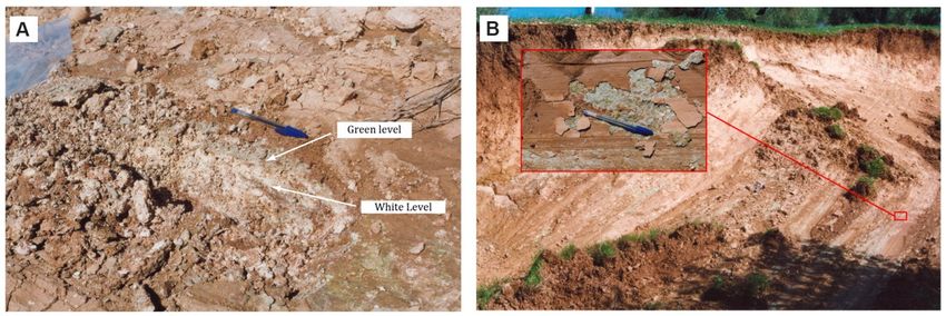
Water 2020, 12, 2639                                                                                                                3 of 24

aquifer, which drains to the south sector. Several springs appear on the contact surface between the
low-permeability flysch-like rocks and the carbonate rocks when the water table in the karstic aquifer
commonly rises after a period of intense rainfall.
     Regarding the hydrogeology of the landslide, three units with varying hydrogeological behaviors
can be distinguished: (i) Carbonate materials from the South Iberian Domain, which have a high
permeability due to karstification; this unit constitutes a free aquifer in which groundwater circulates
through fissures (secondary porosity); (ii) the materials of the Flysch formation, with low permeability
but affected by frequent gravitational movements and colluvial phenomena; and (iii) materials from
the Maláguide Complex, which have a low permeability due to the predominance of clay and slate
materials. However, this formation contains sandstones and conglomerate intercalations with medium
permeability [36].
     The flows provided by carbonate materials, which act as an aquifer in the region, are generally
low (almost never exceed 1 L/s) although they sometimes remain constant as occurs in the spring
located at the head of the landslide, at 1300 m above sea level (point 1 of our sampling, Figures 2 and 3.)
This flow does     not even justify the recharge by direct infiltration of rainwater in the small
           Water 2020, 12, x FOR PEER REVIEW                                                                3 of 24
                                                                                                                    limestone
                                     2
outcrop (less than 10,000 m ) associated with the spring. Therefore, sometimes there must be hidden
           surface between
water connections       between the low-permeability flysch-like
                                      different outcrops         rocks and the
                                                            of materials    or carbonate
                                                                                aquifersrocks
                                                                                         [37].when the water table
             in the karstic aquifer commonly rises after a period of intense rainfall.

            Water 2020, 12, x FOR PEER REVIEW                                                                        4 of 24

            3. Characteristics of the Diezma Landslide
                The Diezma landslide is considered a complex movement affecting an area of 7.76 ha, with a
           maximum length of 510 m and a maximum width of 205 m [32,38]. We divided the landslide body
           into three main sectors (Figure 2):
           1. The landslide head is located on the old Granada–Almería road (CN-342). In this area, several meter-
                scale scarps were observed. These scarps correspond to the shallow rotational slides that have
                developed successively on the clay-rich rocks of the flysch formation. The impermeable characteristic
                of these shear surfaces favored the development of ponds at the foot of the main scarp [11].
           2. The intermediate part of the landslide was formed by progressive rotational slides that produced
                some secondary scarps, which generated bulges with tension cracks at their crests.
           3. The landslide style grades downhill from a multiple rotational slide into a proper earthflow. In
                  Figure 1. Geological sketch of the Betic Cordillera. The study area is outlined by the red rectangle.
                  Geological
       Figure 1.the toe sector, sketch   of theofBetic
                                the thickness           Cordillera.
                                                   the mass  movement   Theinstudy  area area
                                                                              the central  is outlined   by the red
                                                                                                is approximately    30 rectangle.
                                                                                                                        m.
                  Regarding the hydrogeology of the landslide, three units with varying hydrogeological
            behaviors can be distinguished: (i) Carbonate materials from the South Iberian Domain, which have
            a high permeability due to karstification; this unit constitutes a free aquifer in which groundwater
            circulates through fissures (secondary porosity); (ii) the materials of the Flysch formation, with low
            permeability but affected by frequent gravitational movements and colluvial phenomena; and (iii)
            materials from the Maláguide Complex, which have a low permeability due to the predominance of
            clay and slate materials. However, this formation contains sandstones and conglomerate
            intercalations with medium permeability [36].
                  The flows provided by carbonate materials, which act as an aquifer in the region, are generally
            low (almost never exceed 1 L/s) although they sometimes remain constant as occurs in the spring
            located at the head of the landslide, at 1300 meters above sea level (point 1 of our sampling, Figures
            2 and 3.) This flow does not even justify the recharge by direct infiltration of rainwater in the small
            limestone outcrop (less than 10,000 m2) associated with the spring. Therefore, sometimes there must
            be hidden water connections between different outcrops of materials or aquifers [37].
                  As mentioned above, the tectonic structure of the materials brings the clay materials from the
                 Figure
            flysch      2. Geological
                    formation  into    cross-section
                                     contact  with   of the Diezmaaquifer
                                                                    landslide along thelocated
                                                                                         NE-SWat direction. Vertical and we
      Figure 2. Geological
                 horizontal
                               cross-section
                            scales are in meters
                                                  ofthe
                                                     thecarbonate
                                                          Diezma
                                                  (modified from [11]). The
                                                                            materials
                                                                    landslide    along
                                                                            points indicated
                                                                                                   a higher
                                                                                         the correspond
                                                                                              NE-SW       to
                                                                                                              level. Thus,
                                                                                                         direction.
                                                                                                             those of
                                                                                                                       Vertical and
                                                                                                                      theof the
            could assimilate this situation to the existence of a constant hydraulic potential at the head
      horizontalwater
                   scales  are in
                       sampling.   meters   (modified     from  [11]).   The  points   indicated    correspond      to those of the
            slipped zone,   which could favor a certain hidden lateral water supply from the carbonates to the
      water sliding
             sampling.materials, increasing its fluid pressure much more than the simple direct infiltration of
                 The Diezma landslide took place on 18th March 2001, 20 days after a peak in intense rainfall that
            rainwater would have done.
           was preceded by several rainfall episodes, all of which occurred within one year. This year was wetter
                  This hypothesis of a continuous groundwater flow from carbonate materials towards the flysch
           than average [11,32,33,39]. The observed 20-day lag time can be explained by the delay in receiving
            formation outcropping in a lower topographically position helps to explain the time lag between the
           the contribution of groundwater flow from the karst aquifer [32].
            last rainy events and the moment of the slope break [11,37].
                 Immediately after the Diezma landslide occurred, its stabilization began; an additional four lines
           of surface drainage systems and three lines of deep drainage wells were installed, and a barrier of
           anchored piles and a retaining wall at the toe of the slope were constructed [37,40]. In 2002, after the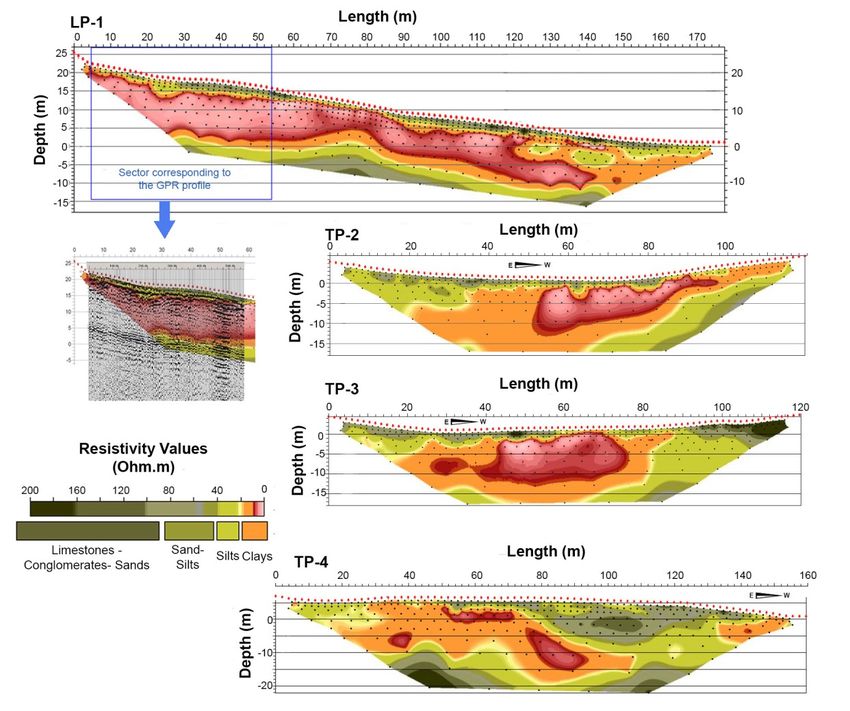
Water 2020, 12, 2639 4 of 24
Water 2020, 12, x FOR PEER REVIEW 6 of 25
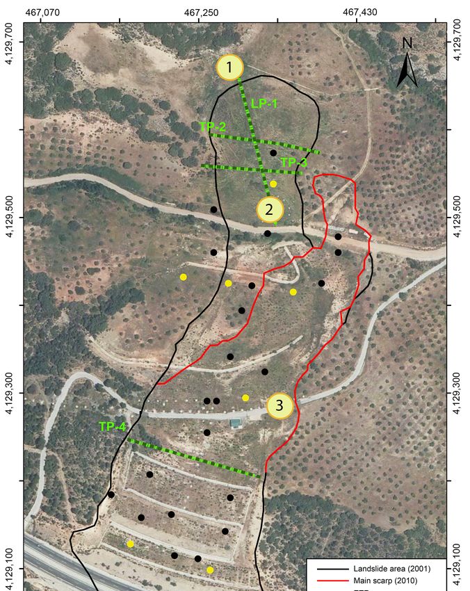
Figure 3.
Figure 3. Aerial view of the Diezma
Diezma landslide.
landslide. The image shows the tracks of the electrical resistivity
resistivity
tomographies and
tomographies and the
the location
location of
of the
the three
three water
water sampling
sampling points.
points. The first
first point
point corresponds
corresponds to to aa
natural upwelling (spring water).
natural upwelling (spring water). The second and the third points were
were taken in depth, in two of the
taken in depth, in two of the
drainage
drainage wells.
wells. The boreholes
boreholes and
and inclinometers
inclinometers carried
carried out
out in
in the
the landslide
landslide are
arealso
alsoshowed.
showed.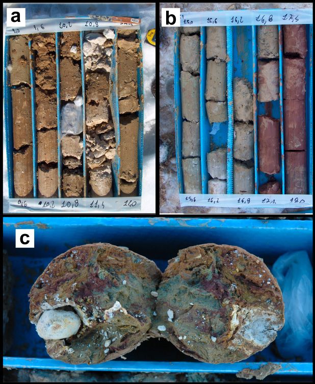
Water 2020, 12, 2639                                                                                 5 of 24

      As mentioned above, the tectonic structure of the materials brings the clay materials from the flysch
formation into contact with the carbonate aquifer materials located at a higher level. Thus, we could
assimilate this situation to the existence of a constant hydraulic potential at the head of the slipped
zone, which could favor a certain hidden lateral water supply from the carbonates to the sliding
materials, increasing its fluid pressure much more than the simple direct infiltration of rainwater would
have done.
      This hypothesis of a continuous groundwater flow from carbonate materials towards the flysch
formation outcropping in a lower topographically position helps to explain the time lag between the
last rainy events and the moment of the slope break [11,37].

3. Characteristics of the Diezma Landslide
     The Diezma landslide is considered a complex movement affecting an area of 7.76 ha, with a
maximum length of 510 m and a maximum width of 205 m [32,38]. We divided the landslide body into
three main sectors (Figure 2):

1.    The landslide head is located on the old Granada–Almería road (CN-342). In this area,
      several meter-scale scarps were observed. These scarps correspond to the shallow rotational slides
      that have developed successively on the clay-rich rocks of the flysch formation. The impermeable
      characteristic of these shear surfaces favored the development of ponds at the foot of the main
      scarp [11].
2.    The intermediate part of the landslide was formed by progressive rotational slides that produced
      some secondary scarps, which generated bulges with tension cracks at their crests.
3.    The landslide style grades downhill from a multiple rotational slide into a proper earthflow.
      In the toe sector, the thickness of the mass movement in the central area is approximately 30 m.

     The Diezma landslide took place on 18th March 2001, 20 days after a peak in intense rainfall that
was preceded by several rainfall episodes, all of which occurred within one year. This year was wetter
than average [11,32,33,39]. The observed 20-day lag time can be explained by the delay in receiving
the contribution of groundwater flow from the karst aquifer [32].
     Immediately after the Diezma landslide occurred, its stabilization began; an additional four lines
of surface drainage systems and three lines of deep drainage wells were installed, and a barrier of
anchored piles and a retaining wall at the toe of the slope were constructed [37,40]. In 2002, after the
stabilization project was completed, a topographic monitoring system was installed that includes
29 benchmarks and 10 inclinometers within the landslide mass [33] (Figure 3).
     However, during field investigations in 2005, it was observed that the water table was very high
in the head area of the Diezma landslide, which indicated that the drainage systems in this zone were
not working properly [41]. Due to this, the Diezma landslide was partially reactivated as a result of the
heavy rainfall that occurred during the winter of December 2009–February 2010.
     Azañón et al. [11] pointed out that the geotechnical characteristics of the material (Table 1) in the
slide mass and those in the slip surface are very different. The landslide debris is heterogeneous in
nature and is mainly composed of sandstone and dolostone blocks embedded in a marl–clay matrix.
These materials were interpreted as a part of a surficial deposit most likely produced by a former
mass movement. On the other hand, the material in the slip surface consists of a centimeter-thick
smectite-rich layer. Thus, the values of the mechanical properties of the mobilized material are
markedly greater than those of the slip surface (Table 1). The smectite-rich layer is highly plastic and
extremely expansive (Table 1). The liquid limits estimated by [11] range from 58 to 92, while the plastic
limits range from 24 to 32. The slide mass has relatively high shear strength values (c = 20 kPa and
φp = 35◦ ). The shear strength in the failure surface is conditioned by residual strength parameters
(c = 39 kPa and φr = 7◦ ). The residual friction angle of the landslide debris is also very low (φr = 20◦ ).
In this landslide, close to the secondary scarp, previous researchers [11] describe that the smectite-rich
levels occur above a powdery white level, consisting of pure calcite with a very small grain size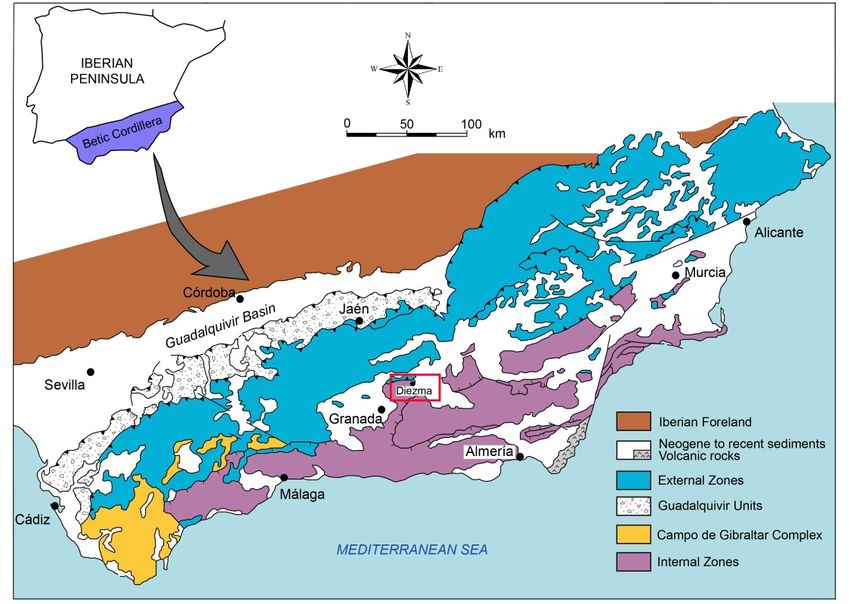
Water 2020, 12, 2639 6 of 24
(Figure 4). Borehole data to which the authors of this paper have had access show that this white level
Waterpresent
is only 2020, 12, xin
FOR
thePEER REVIEW
middle 6 of 24
part of the landslide. On the other hand, the thickness of the smectite-rich
layer increases toward the toe of the landslide.
Table 1. Geotechnical properties of the materials involved in the Diezma landslide (modified from
[11]). The table represents mean values on the 23 samples that have been analyzed on the landslide
Table 1. Geotechnical properties of the materials involved in the Diezma landslide (modified from [11]).
mass and 12 samples on the slip surface.
The table represents mean values on the 23 samples that have been analyzed on the landslide mass and
12 samples on the Parameters
slip surface. Landslide Mass Landslide Slip Surface
Water Content (%) 15 30
Parameters Landslide Mass Landslide Slip Surface
Dry density (g/cm3) 1.7–1.8 1.42–1.59
Water Content
Natural (%) (g/cm3)
density 15 2.1 1.830
Dry density (g/cm 3) 1.7–1.8 1.42–1.59
% Fine grained (8840
Saturation (S) (%)
Limit liquid >9046 >88
80
Limit
Plasticity (%)
liquid index (%) 46 29 5680
Plasticity index (%)
Liquidity Index 29
−0.06 (HOC) 56
0.1 (LOC)
Liquidity Index −0.06 (HOC) 0.1 (LOC)
Classification (USCS) CH-MH CH
Classification (USCS) CH-MH CH
% CaCO% CaCO3 35 35 4–15
4–15
3
ClayClay mineral
mineral composition
composition Smectite
Smectite + illite
+ illite Smectite
Smectite(>90%)
(>90%)
Swelling
Swelling pressure
pressure (kPa)(kPa) 200200 450
450
ϕ’ (pick)/residual 34–36 ◦ /20 19–20/7
φ´ (pick)/residual 34–36°/20 19–20/7
C’ (Kpa)
C´ (Kpa) 20 20 3939
Cc Cc 0.01
0.01 0.02
0.02
Cs 0.0065 0.006
Cs 0.0065 0.006
Figure
Figure 4. 4.
(A)(A) Outcroppicture
Outcrop picturelocated
locatedclose
close to
to the
the secondary
secondary scarp
scarp showing
showingthe thesmectite-rich
smectite-rich thin
thin
layer, which, in turn, overlays a centimeter-thick fine-grained powdery calcite layer, in the slip
layer, which, in turn, overlays a centimeter-thick fine-grained powdery calcite layer, in the slip surface surface
(modified
(modified from
from [11]).(B)
[11]). (B)Secondary
Secondaryscarp
scarpin
inthe
the Diezma
Diezma landslide.
landslide. The
Thebox
boxshows
showsa adetailed
detailed view
view
with slickenside and striations on the landslide slip surface (modified from [11]).
with slickenside and striations on the landslide slip surface (modified from [11]).
To date,
Nieto et al. the
[28]stability problems
determined in the slope of
the proportions have continued,
smectite in thealthough extensive
slide mass and in engineering
the slip zone
measures were applied after the failures in 2001 and 2010. Recently, new monitoring
of the Diezma landslide based on the thermogravimetry of ethylene glycol (EGC)-solvated programssamples.
were
initiated on 2018 due to reactivations in the landslide crown. Moreover, several airborne LiDAR
Their results showed that smectite is the dominant clay mineral in the slip zone, whereas kaolinite
surveys have shown slight deformations in the toe of the slope [42]. This has indicated that the
and illite are minor minerals within the materials of the Diezma landslide. The slip zone has the
stabilization of the Diezma landslide is a complex task in which hydrogeochemical results can be
greatest abundance of clay minerals compared to the materials close to this zone. For this reason,
used to design alternative solutions such as bio-mediated soil improvement methods (cf. [43]).
previous authors [9] suggested that water played a crucial role as a trigger and possibly as a conditioning
factor taking into account the geotechnical and mineralogical characteristics of the materials involved
4. Methodology
in the Diezma landslide.
First, mineralogical and geochemical methods were applied to complete the characterization of
the materials observed in the slip surface. Subsequently, a geophysical survey was carried out to
explore the behavior of groundwater within the landslide mass and its surroundings. Finally, by
integrating all of the gathered information with previously published data, a geochemical simulation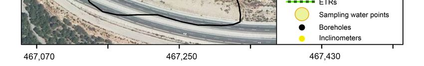
Water 2020, 12, 2639                                                                                   7 of 24

      To date, the stability problems in the slope have continued, although extensive engineering
measures were applied after the failures in 2001 and 2010. Recently, new monitoring programs were
initiated on 2018 due to reactivations in the landslide crown. Moreover, several airborne LiDAR surveys
have shown slight deformations in the toe of the slope [42]. This has indicated that the stabilization
of the Diezma landslide is a complex task in which hydrogeochemical results can be used to design
alternative solutions such as bio-mediated soil improvement methods (cf. [43]).

4. Methodology
     First, mineralogical and geochemical methods were applied to complete the characterization of the
materials observed in the slip surface. Subsequently, a geophysical survey was carried out to explore
the behavior of groundwater within the landslide mass and its surroundings. Finally, by integrating all
of the gathered information with previously published data, a geochemical simulation was developed
to model the water–soil interactions and thus to provide a reasonable explanation for the characteristics
observed in the slip zone.

4.1. Sampling Procedure
     Soil samples were collected from the failure surface. In some outcrops, it was possible to recognize
a level of 1- to 3-cm-thick green clays, corresponding to the most superficial sliding surfaces. In addition,
some samples were taken from the boreholes passing through the landslide. Based on borehole data
and field observations, the main failure surface was found to coincide with a thin layer of clay material,
whereas the mobilized mass comprised marly clay and limestone blocks. The locations of the boreholes
from which the analyzed samples were collected are shown in Figure 3.
     The chemical composition of the water was analyzed at three different points within the Diezma
landslide numbered from 1 to 3: (1) In the spring water located at the edge of the carbonate-marly clay;
(2) above the head of the landslide (at a depth of 11 m); and (3) at the lowest part of the landslide (at a
depth of 27 m) (Figures 2 and 3). Water was sampled in two different seasons (fall and winter) and
after periods of diverse aridity/humidity conditions. Thus, the sampling scheme seeks to represent
not only the chemical composition of groundwater in the slope, but also the effects of climate on the
hydrochemical processes.
     At each water sampling point, pH and conductivity were measured in situ using a HANNA
Instruments HI 9828 Multiparameter. This equipment was checked and calibrated prior to carrying
out the measurements. The concentration of cations in solution was measured using atomic absorption
spectrometry inductively coupled plasma atomic emission spectrometry. The concentrations of anions
(HCO3 − , CO3 and Cl− ) were analyzed by volumetric methods. The concentration of the SO4 ion was
determined using spectrophotometry. For silica analysis, the heteropoly blue (also called olybdate or
molybdenum blue) colorimetric method was employed (ASTM D859).

4.2. Mineralogical Characterization: X-Ray Diffractometry (XRD) and X-Ray Fluorescence (XRF)
     X-ray diffractometry (XRD) is commonly used to analyze clay minerals both qualitatively and
semi-quantitatively. Nevertheless, many factors must be taken into account when performing
quantitative analyses. However, factors related to the semi-quantitative analyses of minerals, such as
the calibration of the diffractometer and the crystallinity, orientation, and heterogeneity of the sample,
are difficult to control. For the XRD analysis, mineralogical changes were studied with a PANanalytical
X’Pert Pro X-ray diffractometer using disoriented powder and samples oriented by the sedimentation of
the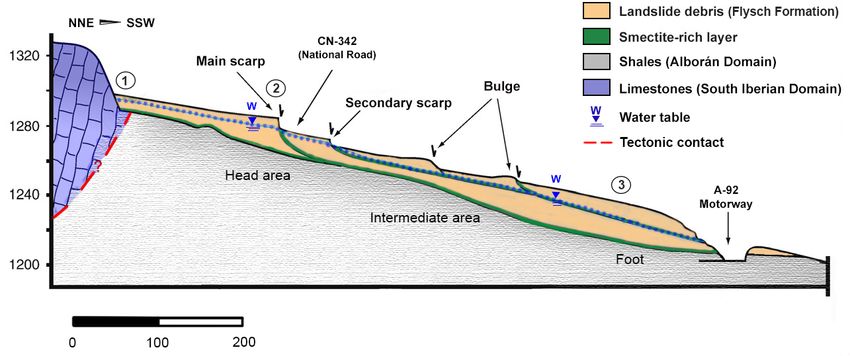
Water 2020, 12, 2639                                                                                   8 of 24

The smectite content was calculated using the following equation: Sme% = 3.96 WL−4.05. For the
X-ray fluorescence spectrometry (XRF) analysis, the fusion method, which is considered one of the
methods with the highest accuracy, was used to determine the bulk chemical composition and relative
abundances of the main components of the landslide materials.

4.3. Geophysical Survey: 2D Electrical Resistivity Tomography (ERT) Profiles
     To identify the water table and the role that water played in the materials involved in the Diezma
landslide, high-resolution 2D electrical resistivity tomography (ERT) was used. Figure 3 shows the
locations of the geoelectrical profiles obtained. Profiles LP-1, TP-2, and TP-3 are located in the head of
the landslide, where the displacement is short and concentrated on a basal surface.
     Profile TP-4 is located in the intermediate and lowest parts of the landslide, where the displacement
is greater and concentrated in numerous scarps [45]. The LP-1 profile starts at the base of the spring
water and extends to the SSE, along 180 m of topographic distance, in an area close to the main scarp.
Profiles TP-2 and TP-3 are developed, from E to W, in the middle and lowest parts of the longitudinal
profile, respectively.
     The equipment employed was a single channel ABEM Terrameter SAS1000. All profiles were
acquired using a Wenner electrode configuration with 61 electrodes connected to a multi-core cable.
The depth of the model depends on the electrode spacing. In the profiles located to the N and 2 m
to the S of the old road, an inter-electrode spacing of 1.5 m was chosen, as it could reach a depth of
18 m with satisfactory resolution. When necessary (i.e., in longitudinal profile), extensions (roll-along
technique) were performed to increase the length of the profile to 1.5, 2 or 2.5× its standard extent.
ERT data were processed using RES2DINV software, which was designed to produce an inverse model
resembling the actual subsurface structure.

4.4. Geochemical Interpretative Methods: Ion-Ion Plots and Geochemical Modelling
     Ion–ion plots were used to infer the possible processes affecting the hydrogeochemical evolution
of the waters. Speciation-solubility, reaction-path, and mass-balance calculations were performed
using the PHREEQC code [46] and the WATEQ4F thermodynamic database [47].
     Inverse modelling was used to calculate the moles of minerals that must dissolve or precipitate
to account for the difference in composition between an initial and a final solution. With that aim,
the number of mineral phases was constrained using inverse modelling, including the potential phases
involved in precipitation or dissolution processes based on a conceptual model. This model was
inferred based on the general trends in the water chemical data and the saturation indices of the waters
with respect to different mineral phases.

5. Results

5.1. Mineralogical Characteristics of the Slip Zone
      The XRF (X-ray fluorescence) results reveal that the slip zone contains high concentrations of SiO2 ,
Al3+ , K+ , Mg2+, and Ca2+ , as well as lower concentrations of Na+ (Table 2). This may indicate that the
slip zone is rich in clay minerals.
      From the XRD (X-ray diffractometry) diagrams, the main mineralogical associations were
established. The powder sample diagram shows that the landslide-slip zone materials are mainly
composed of quartz, clay minerals, calcite, and dolomite (Figure 5). Chlorite and micas (muscovite and
paragonite) are also present in lesser proportions. The oriented sample (
Water 2020, 12, x FOR PEER REVIEW                                                                        9 of 24

             Table 2. Concentrations (in % and ppm) of the major and minor elements identified in the XRF
             analysis. The table represents mean values on XRF tests that have been performed on seven samples.
Water 2020, 12, 2639                                                                                                9 of 24
                              Compound              (%)         Element           Ppm
                                 SiO2              64.23           O             527300
     Table 2. Concentrations (in Al
                                 %2Oand
                                      3 ppm) of the13.15
                                                     major and minor
                                                                   Si elements identified
                                                                                 300300   in the XRF analysis.
                                 H2 O              9.63            Al             69610
     The table represents mean values on XRF tests that have been performed on       seven samples.
                                 Fe2O3             6.05            Fe             42320
                                  K2O              2.925           K              24280
                        Compound MgO
                                             (%) 2.121       Element
                                                                   Mg
                                                                                 Ppm
                                                                                  12790
                            SiO2 CaO        64.230.814          O H               10780
                                                                               527,300
                           Al2 O3TiO2       13.150.665          Si Ca             5820
                                                                               300,300
                                 Na2O              0.197           Ti             3980
                            H2 O             9.63               Al              69,610
                                 P2O5              0.068           Na             1460
                           Fe2 O3MnO         6.05 0.0308        Fe P            42,320
                                                                                   300
                            K2 O SO3        2.925 0.02          K Mn            24,280
                                                                                   238
                           MgOCr2O3         2.1210.019         MgCr             12,790
                                                                                   135
                            CaO CuO         0.8140.0153         H Cu            10,780
                                                                                   122
                            TiO2 ZnO        0.6650.014          Ca Rb              122
                                                                                 5820
                                 Rb2O             0.0133           Zn              113
                           Na2 O            0.197               Ti               3980
                                  SrO            0.00922            S               81
                           P2 O5 NiO        0.0680.00907        Na Sr            1460
                                                                                    78
                           MnOGa2O3        0.03080.0026         P Ni              300
                                                                                    71
                            SO3 Y2O3         0.020.00202       MnGa               238
                                                                                    19
                           Cr2 O3           0.019               Cr Y              135
                                                                                    16
                            CuO               0.0153              Cu                 122
           From the XRD (X-ray
                            ZnO diffractometry)0.014 diagrams, Rb  the main mineralogical
                                                                                     122        associations were
      established. The powder
                           Rb2 O sample  diagram
                                              0.0133 shows  that the
                                                                  Zn  landslide-slip zone
                                                                                     113    materials   are mainly
      composed of quartz, clay
                            SrO   minerals, calcite,
                                             0.00922  and dolomite  S(Figure 5). Chlorite
                                                                                     81    and   micas  (muscovite
      and paragonite) are also
                            NiOpresent in lesser  proportions. TheSroriented sample78
                                             0.00907                                   (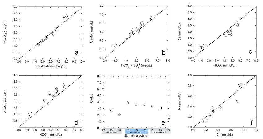
5.2. Internal Geometry and Groundwater Flow in the Diezma Landslide
       The ERT profiles carried out in the Diezma landslide show areas of high conductivity (with
 resistivity values of
Water 2020, 12, 2639 11 of 24
Water 2020, 12, x FOR PEER REVIEW 11 of 24
Figure7. 7.Resistivity
Figure sections
Resistivity for electrical
sections resistivity
for electrical tomography
resistivity (ERT) profiles
tomography (ERT) at the Diezma
profiles landslide.
at the Diezma
The tomography study was performed in the winter season.
landslide. The tomography study was performed in the winter season.
5.3. Groundwater Hydrochemistry in the Diezma Landslide
In the longitudinal profile (LP-1), the abrupt change in resistivity at the southern end of the
Water
profile chemistrymore
is attributed can beto aused as aeffect
drying tool caused
to identify thedrainage
by the processes and mechanisms
borehole affectinginthe
than to a variation the
groundwater
clay composition. (e.g., [48–50]).
Thus, theTherefore,
resistivity the groundwater
values are strongly composition
affected byand the mineralogy
degree of soil ofmoisture.
the different
The
rocks
lowest present in the
resistivity area have
values (below been usedbelong
10 Ω.m) to determine
to thosethe source of
materials the
that major
are closeions
to theinsaturation
the water state.
and
their
The relations
substratewith of theweathering
Maláguideprocesses.
contact is located in the deepest part of the profile and has a value of
The groundwater in the 2+ -HCO − type (Table 3 and Figure 8), with Ca
20 Ω.m. From this point on,landslide
there is aissignificant
generally Ca increase in3the resistivity gradient. This contact is
ranging from by 1.51 −
also revealed thetooverlap
2.53 mmol/L and HCO3 ranging
of a ground-penetrating from section
radar (GPR) 3.39 to with
5.95 the
mmol/L. In general,
coincident resistive
chemical
field, where analyses show increases
the resistive in Ca2+ , Mgto
gradient corresponds 2+ , alkalinity, and total dissolved solids (TDS) as
the deep reflective layer (Figure 7).
the waterIn themoves from points
intermediate 1 to 3 (see
profiles, theFigure
area 3).
with Taking
lowerinto account the
resistivity in mineralogy
the central of the aquifer
sector should
rocks, the concentrations
correspond to a channelofwhere the dissolved major elements
water circulated, thus appear to bethat
indicating determined by the
its materials aredissolution
saturated.ofIn
carbonate mineralsTP-4,
(e.g.,the
calcite and dolomite), which contributes Ca2+ , Mg2+ ,such −
the last profile, resistivity gradient is located at thethe observed
bottom of the profile, and HCO
that 3the
toisolines
the water.of 20 and 40 Ω.m are slightly separated. This information, when correlated with the borehole
data, Asallows
mentioned
us to above,
set the ion–ion plots (see
sliding level Figure
between 9) were
these used to infer the possible processes affecting
isolines.
the hydrogeochemical evolution of the studied waters (e.g., [51]). The values of Ca2+ + Mg2+ versus
5.3. Groundwater
total cations (Figure Hydrochemistry
9a) lie alonginathe 1:1Diezma Landslide that Ca2+ and Mg2+ are the main cations
line, suggesting
present in thechemistry
waters. When + and/or
Water can bedatauseddeviate
as a toolfrom
to that line,the
identify it indicates
processesthat
andother cations (Na
mechanisms affecting the
+
Kgroundwater
) contribute(e.g.,substantially to the water 2+ + Mg 2+ +
[48–50]). Therefore, thechemistry.
groundwater Thecomposition
plot of Ca and versus of
mineralogy bicarbonate
the different
sulfate (Figure in
rocks present 9b)the
shows
area that,
havein general,
been used most of the points
to determine fall along
the source of thethemajor
equiline,
ions which indicates
in the water and
that the Ca 2+ and Mg2+ chemistry is largely explained by carbonate and sulfate weathering processes.
their relations with weathering processes.
The points that fall on theinCa 2+ and Mg2+ side indicate excess Ca and Mg derived from other processes,
The groundwater the landslide is generally Ca2+-HCO3− type (Table 3 and Figure 8), with Ca
such as ion exchange reactions [48].
ranging from 1.51 to 2.53 mmol/L and HCO3− ranging from 3.39 to 5.95 mmol/L. In general, chemical
analyses show increases in Ca2+, Mg2+, alkalinity, and total dissolved solids (TDS) as the water moves from
points 1 to 3 (see Figure 3). Taking into account the mineralogy of the aquifer rocks, the concentrations of
the dissolved major elements appear to be determined by the dissolution of carbonate minerals (e.g.,
calcite and dolomite), which contributes the observed Ca2+, Mg2+, and HCO3− to the water.(mmol/L) Gy Hal
L) l l h
- - -
7.7 2.0 0.0 0.3 0.1 n.m 0.0 0.2 0.6 0.6
P1 4.55 6.2 385 2.9 3.1 9.0
7 5 1 3 7 . 4 2 6 7
5 7 9
- - -
8.1 1.5 0.0 0.5 0.3 n.m 0.4 0.3 0.7 1.2
October 11 P2 3.39 2.6 339 1.9 2.2 8.6
7 1 1 8 0 . 5 3 9 9
Water 2020, 12, 2639 9 1 7 12 of 24
- - -
8.0 1.7 0.0 0.8 0.3 n.m 0.3 0.4 0.8 1.5
P3 4.15 2.1 397 2.0 2.2 8.4
9 5 1 2 8 . 6 3 5 0
7 9 5
Table 3. Chemical composition of the groundwater 7.5
in the
2.0
Diezma
0.0 0.5
landslide
0.1 n.m
in the
0.0
different
0.1
sampling campaigns.
0.5
The
0.5
table
- also- shows- some calculations such as the
P1 5.00 3.9 427 2.6 2.8 9.4
Ca/Mg ratio, the TDS (total dissolved solids), and6 the 8saturation
0 3 indices
2 with
. respect
8 5 the main mineral phases 0 such 4 as calcite (Cal), dolomite (Dol), gypsum (Gy),
3 5 0
anhydrite (Anh), and halite (Hal), n.m.: not measured. - - -
February 7.8 2.5 0.0 0.7 0.2 n.m 0.3 0.2 0.9 1.4
P2 5.95 3.6 529 1.9 2.1 8.9
13 9 3 2 0 2 . 7 6 4 6
Ca K Mg Na SiO2 SO4 Cl HCO3 − TDS 4 6 2 Saturation Indices
Date Sample pH Ca/Mg
(mmol/L) (mg/L) - Cal - -
Dol Gy Anh Hal
8.0 1.7 0.0 0.8 0.3 n.m 0.4 0.3 0.9 1.4
P3 4.40 2.1 421 1.9 2.1 8.9
P1 7.77 2.05 0.01 20.33 2 0.172 4
n.m. 8 0.04. 9
0.22 0 4.55 6.2 5 385 7 0.66 0.67 −2.95 −3.17 −9.09
3 5 2
October 11 P2 8.17 1.51 0.01 0.58 0.30 n.m. 0.45 0.33 3.39 2.6 339 0.79 1.29 −1.99 −2.21 −8.67
- - -
P3 8.09 1.75 0.01 0.82 1.8 0.38
7.8 0.0 n.m. 0.2 0.36
0.5 0.3 0.43 0.2 4.15
0.0 2.1 0.7 3971.0 0.85 1.50 −2.07 −2.29 −8.45
P1 4.75 3.4 398 2.8 3.0 8.9
5 8 0 6 1 2 6 7 2 4
P1 7.56 2.08 0.00 0.53 0.12 n.m. 0.08 0.15 5.00 3.9 427 2 0.50 4 0.54
2 −2.63 −2.85 −9.40
February 13 P2 7.89 2.53 0.02 0.70 0.22 n.m. 0.37 0.26 5.95 3.6 529 - 0.94 - 1.46
- −1.94 −2.16 −8.92
P3 8.02 November
1.72 0.02 7.9
0.84 2.2 0.0
0.38 0.7
n.m. 0.3 0.4
0.49 0.4
0.30 0.3 4.40 0.8 1.3 −1.93 −2.15 −8.92
P2 5.00 3.1 2.1 473 421 1.90.95 2.1 1.47
8.6
14 1 3 3 2 2 8 4 2 4 3
P1 7.85 1.88 0.00 0.56 0.21 0.32 0.06 0.27 4.75 3.4 398 0 0.72 2 6
1.04 −2.82 −3.04 −8.92
November 14 P2 7.91 2.23 0.03 0.72 0.32 0.48 0.44 0.32 5.00 3.1 473 - 0.84 - 1.33
- −1.90 −2.12 −8.66
7.9 1.8 0.0 1.1 0.5 0.8 0.3 0.7 0.7 1.4
P3 7.90 1.80 0.00
P3 1.11 0.50 0.80 0.30 0.70 5.10
5.10 1.6 1.6 473 473 2.10.75 2.3 1.43
8.1 −2.16 −2.38 −8.12
0 0 0 1 0 0 0 0 5 3
6 8 2
Representation
Figure 8.Figure of the composition
8. Representation of the water
of the composition of the samples obtained
water samples in thisin
obtained study in a Piper–Hill
this study in a Piper–diagram.
Hill diagram.
As mentioned above, ion–ion plots (see Figure 9) were used to infer the possible processes
affecting the hydrogeochemical evolution of the studied waters (e.g., [51]). The values of Ca2+ + Mg2+
versus total cations (Figure 9a) lie along a 1:1 line, suggesting that Ca2+ and Mg2+ are the main cationspresent in the waters. When data deviate from that line, it indicates that other cations (Na and/or K )
contribute substantially to the water chemistry. The plot of Ca2+ + Mg2+ versus bicarbonate + sulfate
(Figure 9b) shows that, in general, most of the points fall along the equiline, which indicates that the
Ca2+ and Mg2+ chemistry is largely explained by carbonate and sulfate weathering processes. The
points that fall on the Ca2+ and Mg2+ side indicate excess Ca and Mg derived from other processes,
Water 2020, 12, 2639 13 of 24
such as ion exchange reactions [48].
Figure Correlation diagrams
Figure 9.9. Correlation diagrams between
between CaCa ++ Mg Mg and
and total cations
cations (a),
(a), CaCa ++ Mg
Mg and
and
bicarbonate+sulphate (b); Ca
bicarbonate+sulphate (b); Ca and
andbicarbonate
bicarbonate(c); Ca+ +
(c);Ca MgMg and
and bicarbonate
bicarbonate (d);(d); Ca/Mg
Ca/Mg ratios
ratios of
of the
the sampling points (e) (background colors indicate different dates); and Na and
sampling points (e) (background colors indicate different dates); and Na and Cl (f). Cl (f).
Waters derivedfrom
Waters derived fromcalcite
calcite or dolomite
or dolomite dissolution
dissolution normallynormally
lie above liethe
above theon2:1
2:1 line theline on the
bicarbonate
bicarbonate versus Ca plot and the bicarbonate versus Ca 2+ + Mg2+ plot, respectively ([52,53];
versus Ca plot and the bicarbonate versus Ca2+ + Mg2+ plot, respectively ([52,53]; Figure 9c,d). The results
Figure 9c,d).
show that some Theofresults show that
the samples some the
lie above of the2:1samples lie above
line, indicating thatthethey2:1 originated
line, indicatingfrom that they
carbonate
originated from carbonate dissolution. However, there is a group of samples
dissolution. However, there is a group of samples that do not fall above the 2:1 line, which suggests that that do not fall above the
2:1 line, which suggests that Ca 2+ and Mg2+ are involved in additional geochemical processes other
Ca2+ and Mg2+ are involved in additional geochemical processes other than carbonate dissolution (e.g.,
than
ioniccarbonate
exchange dissolution
processes). The(e.g.,Caionic
2+/Mg exchange
2+ ratios of processes).
the watersThe Ca2+/the
support
2+ ratios of the waters support
Mghypothesis of the dissolution of
the hypothesis
carbonates of theprocess
as a main dissolution of carbonates
in the studied systemas a main
(Figure 9e,process
Table 3).inIf the
the Ca studied
2+/Mg2+system (Figure
molar ratio 9e,
is equal
Table 3). If the Ca 2+/ Mg2+ molar ratio is equal to one, the dissolution of dolomite should occur [54],
to one, the dissolution of dolomite should occur [54], whereas higher ratios, such as the ratios from our
whereas higher
waters, are ratios, such
indicative of a as the ratios
greater calcitefrom our waters,Previous
contribution. are indicative of a greater
researchers [55] alsocalcite contribution.
explained that a
Previous researchers [55] also explained that a higher Ca 2+/ Mg2+ molar ratio (>2) is indicative of the
higher Ca2+/Mg2+ molar ratio (>2) is indicative of the dissolution of silicate minerals.
dissolution
Finally, of it
silicate minerals.to highlight the good 1:1 correlation between the molar dissolved
is important
Finally, it is important
concentrations of Na+ and Cl to− highlight
in most ofthe thegood 1:1 correlation
studied waters (Figure between the molar that
9f), suggesting dissolved
halite
concentrations of Na + and Cl− in most of the studied waters (Figure 9f), suggesting that halite
dissolution is the main source of Na+ and Cl− in the system [50]. Those values that deviate from the
dissolution is thethat
1:1 line indicate mainthesource of Na+ and Cl
Na concentration
− in the system [50]. Those values that deviate from the
is involved in ion exchange processes and that Na+ and Cl−
1:1 line indicate that the Na concentration
concentrations do not increase simultaneously. is involved in ion exchange processes and that Na+ and Cl−
concentrations
Saturationdo not increase
indices are also simultaneously.
useful for evaluating and supporting the processes deduced from
Saturation indices are also
ion–ion plots. Then, the saturation indices useful for evaluating
of the mainand supporting
minerals the processes
controlling the waterdeduced
chemistry from
can
ion–ion plots. Then, the saturation indices of the main minerals controlling
be calculated using PHREEQC (Table 3). The saturation index (SI) indicates whether a solution is the water chemistry canin
be calculated using PHREEQC (Table 3). The saturation index (SI) indicates
equilibrium (SI = 0), undersaturated (0) with respect to a solid phase. In whether a solution is in
equilibrium (SI = 0), undersaturated
practice, equilibrium can be assumed (0) with respect
to +0.05 [56].toIfawater
solid phase. In practice,
is undersaturated
equilibrium can be assumed to span a range of −0.05 to +0.05 [56].
with respect to a given mineral, then that mineral would dissolve if it were present in the system.If water is undersaturated with
respect
However,to asupersaturation
given mineral, then is not that mineral would
equivalent dissolve ifIfitprecipitation
to precipitation. were presentkinetics in the system.
is slow,However,
solutions
supersaturation is not equivalent to precipitation. If precipitation
can remain supersaturated and not precipitate with regard to a mineral phase for a long time kinetics is slow, solutions can remain
[56].
supersaturated and not precipitate with regard to a mineral phase for a long time [56].
The results of the calculated saturation indices (Table 3) revealed that the waters are undersaturated
with respect to halite, gypsum, and anhydrite and are close to equilibrium or slightly oversaturated
with respect to calcite and dolomite. This indicates that halite and gypsum (or anhydrite) will dissolve,
which is consistent with the results of the ion-ion plots (Figure 9b,f). The obtained values for calcite
and dolomite, together with the results of the ion–ion plots, suggest that they could be dissolved.Water 2020, 12, x FOR PEER REVIEW 14 of 24
The results of the calculated saturation indices (Table 3) revealed that the waters are
undersaturated with respect to halite, gypsum, and anhydrite and are close to equilibrium or slightly
oversaturated
Water 2020, 12, 2639 with respect to calcite and dolomite. This indicates that halite and gypsum (or
14 of 24
anhydrite) will dissolve, which is consistent with the results of the ion-ion plots (Figure 9b,f). The
obtained values for calcite and dolomite, together with the results of the ion–ion plots, suggest that
However, dolomite dissolves much more slowly than calcite [57–59]; therefore, its dissolution is
they could be dissolved. However, dolomite dissolves much more slowly than calcite [57–59];
less plausible.
therefore, its dissolution is less plausible.
Another tool used to test the hydrochemical evolution of groundwater is stability diagrams,
Another tool used to test the hydrochemical evolution of groundwater is stability diagrams,
which can be used to help define the reactions that control water chemistry. However, especially in
which can be used to help define the reactions that control water chemistry. However, especially in
clays, there are some sources of uncertainty in setting the boundaries between these phases in stability
clays, there are some sources of uncertainty in setting the boundaries between these phases in stability
diagrams (e.g., experimental measurements, inconsistencies introduced from standard free-energies,
diagrams (e.g., experimental measurements, inconsistencies introduced from standard free-energies,
and differences in the properties of the mineral phases [60]). Therefore, we constructed a diagram
and differences in the properties of the mineral phases [60]). Therefore, we constructed a diagram
using different equilibrium constants obtained from the literature for the following reaction:
using different equilibrium constants obtained from the literature for the following reaction:
6 Ca-Montmorillonite + 2 H++2+H23
6 Ca-Montmorillonite + +H H=
232 O 2O7=Kaolinite + Ca
7 Kaolinite 2+ 2+
+ Ca + +8 8HH
4 SiO
4SiO
44 (1)
(1)
Thevalues
The valuesused
used here
here are
are loglog
K=K −15.7,
= −15.7, log
log KK= =−18.4
−18.4±±0.8
0.8and
andlog
logKK==−16.3
−16.3±±1,1,which
whichcorrespond
correspond
to those proposed by [61–63], respectively. The results (Figure 10) show that when
to those proposed by [61–63], respectively. The results (Figure 10) show that when considering theconsidering the
uncertaintiesofofthe
uncertainties theconstants
constantsandandthe
thedifferent
differentreported
reportedvalues,
values,the
thethree
threesamples
samplesplot
plotvery
veryclose
closetoto
the equilibrium line, suggesting that one mineral is dissolving incongruently and resulting ininthe
the equilibrium line, suggesting that one mineral is dissolving incongruently and resulting the
formation of the other.
formation of the other.
Figure 10. Stability diagram plot to evaluate the water composition in terms of water–rock equilibrium.
Figure 10. Stability diagram plot to evaluate the water composition in terms of water–rock
The triangle, circle, and diamond correspond to points 1, 2, and 3, respectively, of the November 2014
equilibrium. The triangle, circle, and diamond correspond to points 1, 2, and 3, respectively, of the
sampling campaign.
November 2014 sampling campaign.
5.4. Process Quantification by Mass-Balance Calculations
5.4. Process Quantification by Mass-Balance Calculations
The analyses of the hydrochemical trends for the main elements of the system, together with
The analyses of
speciation-solubility the hydrochemical
calculations trends diagram
and the stability for the main
of theelements of the
clays, allow system,
us to deduce together with
the general
speciation-solubility calculations and the stability diagram of the clays, allow us to
geochemical processes that could control the composition of the water. Therefore, based on the chemicaldeduce the general
geochemical
data and field processes
mineralogicalthat observations,
could control itthe composition
is proposed thatofthethemain
water. Therefore,processes
geochemical based onare the
chemical
the dataorand
dissolution field mineralogical
precipitation observations,
of calcite, halite, gypsum,itquartz,
is proposed that
kaolinite, andthe main geochemical
Ca-montmorillonite,
processes are the dissolution or precipitation of calcite, halite, gypsum,
as well as cationic exchange reactions. Mass-balance and reaction-path simulations were quartz, kaolinite,
carriedand
out Ca-
to
montmorillonite,
quantify the relativeasimportance
well as cationic exchange
of those reactions.
processes Mass-balance
along the andfrom
flow path (i.e., reaction-path simulations
point 1 to point 2 and
werepoint
from carried
2 toout to quantify
point 3). the relative importance of those processes along the flow path (i.e., from
pointMass-balance models, used in2geochemistry
1 to point 2 and from point to point 3). to evaluate the chemical transfers between phases
Mass-balance
in water models, are
(e.g., [51,64–66]), usedbased
in geochemistry to evaluate
on the principle that the chemical
if one watertransfers
evolved between phases
from another,
in water (e.g., [51,64–66]), are based on the principle that if one water evolved
the compositional differences can be accounted for by the minerals and gases that leave or enter that from another, the
packet of water [67] within specified compositional uncertainty limits:
initial water + reactants → final water + products (2)Water 2020, 12, x FOR PEER REVIEW 15 of 24
Water 2020, 12, 2639differences
compositional 15 of
can be accounted for by the minerals and gases that leave or enter 24
that
packet of water [67] within specified compositional uncertainty limits:
An uncertainty limit ofinitial
0.05 (5%)
waterwas adjusted
+ reactants forfinal
all ofwater
the analytical
+ productsdata used in our modelling
(2)
calculations, and then PHREEQC considers these uncertainties analyses to solve alkalinity-balance
An uncertainty limit of 0.05 (5%) was adjusted for all of the analytical data used in our modelling
and element concentration-balance. These models are not unique; therefore, they were constrained
calculations, and then PHREEQC considers these uncertainties analyses to solve alkalinity-balance
based on the bulk mineralogical composition of the soil and the hydrogeochemical trends observed
and element concentration-balance. These models are not unique; therefore, they were constrained
in the system. The plausible phases included in the model are calcite, gypsum, halite, kaolinite,
based on the bulk mineralogical composition of the soil and the hydrogeochemical trends observed
Ca-montmorillonite, quartz, CO2 , and CaX2 , NaX, and MgX2 species for ionic exchange reactions of Ca
in the system. The plausible phases included in the model are calcite, gypsum, halite, kaolinite, Ca-
or Mg for Na on exchange sites. For those plausible phases, the chemical evolution of the water along
montmorillonite, quartz, CO2, and CaX2, NaX, and MgX2 species for ionic exchange reactions of Ca
the water path is constrained by relationships of conservation of mass. The equations to calculate the
or Mg for Na on exchange sites. For those plausible phases, the chemical evolution of the water along
mass transfer coefficients (αphase ) are the following:
the water path is constrained by relationships of conservation of mass. The equations to calculate the
mass transfer coefficients (αphase
∆ m , Ca = α) are the
+ αfollowing:
gypsum + α +α (3)
T calcite Ca-montmorillonite Ca-exchange
∆ mT, Ca = αcalcite + αgypsum + αCa-montmorillonite + αCa-exchange (3)
∆ mT , Na = αhalite + αNa-exchange (4)
∆ mT, Na = αhalite + αNa-exchange (4)
∆ mT , C = αcalcite + αCO2 (5)
∆ mT, C = αcalcite + αCO2 (5)
∆ mT , SO4 2− = αgypsum (6)
∆ mT, SO42- = αgypsum (6)
∆ mT , Cl = αhalite (7)
∆ mT, Cl = αhalite (7)
∆ mT , Mg = αMg-exchange (8)
∆ mT, Mg = αMg-exchange (8)
∆ mT , SiO2 = αquartz + αkaolinite + αCa-montmorillonite (9)
∆ mT, SiO2 = αquartz + αkaolinite + αCa-montmorillonite (9)
where ∆ mT are the change in total moles of an element in solution along the flow path (final water
where ∆ mT are the change in total moles of an element in solution along the flow path (final water
minus initial water).
minus initial water).
The summary of the best modelling results obtained here is shown in Figure 11. The mass-balance
The summary of the best modelling results obtained here is shown in Figure 11. The mass-
results suggest that geochemical processes involving carbonates, gypsum, halite, kaolinite, quartz,
balance results suggest that geochemical processes involving carbonates, gypsum, halite, kaolinite,
and Ca-montmorillonite, as well as ion exchange reactions, control the water chemistry; this is consistent
quartz, and Ca-montmorillonite, as well as ion exchange reactions, control the water chemistry; this
with the results of the ion-ion analysis and the observed chemical trends.
is consistent with the results of the ion-ion analysis and the observed chemical trends.
Figure
Figure 11. Mass-balance
11. Mass-balance models
models from
from point
point 1 to 2point
1 to point 2 (A),
(A), and fromand from
point 2 topoint
point 32(B)
to of
point 3 (B) of
the landslide.
the landslide.
The rainfall occurring in the months close to the sampling could have some influence on the
The rainfall occurring in the months close to the sampling could have some influence on the
dissolution and/or precipitation of different mineral phases. The first water sampling was carried out
dissolution and/or precipitation of different mineral phases. The first water sampling was carried out
in October 2011, the second sampling was performed in February 2013, and the final sampling was
in October 2011, the second sampling was performed in February 2013, and the final sampling was
performed in November 2014. Some differences in terms of recorded rainfall are observed between
performed in November 2014. Some differences in terms of recorded rainfall are observed betweenWater 2020, 12, 2639 16 of 24
Water 2020, 12, x FOR PEER REVIEW 16 of 24
thesethree
these threeyears.
years.We
We collected
collected pluviometric
pluviometric data
data from
from thethe nearest
nearest measurement
measurement station
station to analyze
to analyze the
the amount
amount of precipitation
of precipitation recorded
recorded in theinthree
the three months
months beforebefore each sampling
each sampling (Figure
(Figure 12). 12).
Figure12.12.Cumulative
Figure Cumulativerainfall (mm)
rainfall in the
(mm) inthree
the months prior toprior
three months each sampling, including including
to each sampling, the sampling
the
month (accumulated
sampling precipitation
month (accumulated is measuredisinmeasured
precipitation mm). in mm).
Thus,
Thus,ititcan
canbebeobserved
observedthat thatthe
thefirst
firstsampling
samplingyear
yearwaswasthethedriest;
driest;only
onlyprecipitation
precipitationduring
duringthethe
month
month of sampling is registered. However, the accumulated precipitation is quite high in almostall
of sampling is registered. However, the accumulated precipitation is quite high in almost all
ofofthe
themonths
monthspriorpriortotothe
thesecond
secondsampling.
sampling.Finally,
Finally,inin2014,
2014,the
thecumulative
cumulativeprecipitation
precipitationincreases
increases
gradually,
gradually,with witha avalue
valueofofzero
zeroininthe
thethird
thirdmonth
monthprior
priortotosampling
samplingand andhigh
highvalues
values(You can also read