The role of skills and tasks in changing employment trends and income inequality in Chile - WIDER Working Paper 2021/48

WIDER Working Paper 2021/48

The role of skills and tasks in changing
employment trends and income inequality in
Chile

Gabriela Zapata-Román*

March 2021

Abstract: Using decomposition methods, we analyse the role of the changing nature of work in
explaining changes in employment, wage inequality, and job polarization in Chile from 1992 to
2017. Changes in occupational structure confirm a displacement of workers from low-skill
occupations towards jobs demanding non-routine higher skills (professionals and technicians), and
to jobs demanding routine manual and cognitive tasks (services and sales). Changes in occupational
earnings have had an equalizing effect, with more substantial gains in favour of lower-skill
occupations and also at the top of the skill premium. Inequality reductions since the 2000s are
explained by a fall in earnings in the top percentiles of the distribution, which have been reallocated
most noticeably around the median (2000–06) and the bottom 30 per cent (2006–17). Changes in
the returns to education and the relocation of workers towards less-routine occupations have
contributed to the inequality reduction.
Key words: wage inequality, job polarization, skills, tasks, decomposition methods, Chile
JEL classification: J23, J24, J31, J6, O33
Acknowledgements: The author is grateful for valuable feedback on previous versions of this
paper from the internal and external UNU-WIDER research team, collaborating under the project
‘The changing nature of work and inequality’, and particularly for the comments from Carlos
Gradín, Simone Schotte, and Piotr Lewandowski.
Note: The Technical Appendix is available here (https://www.wider.unu.edu/publication/role-
skills-and-tasks-changing-employment-trends-and-income-inequality-chile).

* Global Development Institute, The University of Manchester, United Kingdom, gabriela.zapataroman@manchester.ac.uk
This study has been prepared within the UNU-WIDER project The changing nature of work and inequality.
Copyright © UNU-WIDER 2021
UNU-WIDER employs a fair use policy for reasonable reproduction of UNU-WIDER copyrighted content—such as the
reproduction of a table or a figure, and/or text not exceeding 400 words—with due acknowledgement of the original source,
without requiring explicit permission from the copyright holder.
Information and requests: publications@wider.unu.edu
ISSN 1798-7237 ISBN 978-92-9256-986-0
https://doi.org/10.35188/UNU-WIDER/2021/986-0
Typescript prepared by Luke Finley.
United Nations University World Institute for Development Economics Research provides economic analysis and policy advice
with the aim of promoting sustainable and equitable development. The Institute began operations in 1985 in Helsinki, Finland, as
the first research and training centre of the United Nations University. Today it is a unique blend of think tank, research institute,
and UN agency—providing a range of services from policy advice to governments as well as freely available original research.
The Institute is funded through income from an endowment fund with additional contributions to its work programme from
Finland, Sweden, and the United Kingdom as well as earmarked contributions for specific projects from a variety of donors.
Katajanokanlaituri 6 B, 00160 Helsinki, Finland
The views expressed in this paper are those of the author(s), and do not necessarily reflect the views of the Institute or the United
Nations University, nor the programme/project donors.

1 Introduction

A key issue in development economics has been to understand the effects of technological changes
in the labour market, in terms of their impact on both wage inequality and job creation and
destruction. The literature of the late 1990s suggested that technological change was skill-biased
and would favour high-skill workers and replace routine tasks. Skill-biased technological change
(SBTC) increases the marginal productivity of skilled labour in relation to unskilled labour, and
consequently its demand and salary premium, which leads to an increase in wage inequality (Berman
et al. 1998).

More recent literature has built on Autor et al.’s (2003) hypothesis, which argues that technological
change has two effects on labour markets: first, it replaces workers in performing routine cognitive
and manual tasks that can be achieved by following explicit rules (which can be automated); second,
it complements workers in the performance of non-routine problem solving and complex
communications. Therefore, technological change will lead to a lower demand not necessarily for
all low-skilled workers, only for those involved in routine tasks that can now be replaced with the
use of technology. At the same time, this can lead to a greater demand for workers whose tasks are
complementary to computerization, such as people who work in occupations where non-routine
cognitive skills are required (Acemoglu and Restrepo 2017), which are generally measured at the
occupational level (Firpo et al. 2011).

The relative share of cognitive and manual routine jobs has declined over time in the US and other
developed economies (Autor et al. 2003; Goos et al. 2014; Jensen and Kletzer 2010; Michaels et al.
2013), contributing to wage polarization and therefore higher levels of inequality. While this is true
for advanced economies, there is evidence suggesting that developing countries and emerging
economies are not following the same trends. Surveys in China and some Central and Eastern
European countries show that the proportion of people employed in routine-intensive occupations
has increased in recent decades (Du and Park 2017; Hardy et al. 2018).

Inequality trends also behave differently in developing countries. While most of the developed
world has experienced rising inequality since the 2000s, most countries in Latin America have
followed the opposite pattern. Messina and Silva (2019) argue that the absence of skill-biased
technological change and little evidence of job polarization in Latin America have facilitated the
decline of wage inequality in the region. They found that wages expanded rapidly in low-paying
occupations relative to high-paying occupations, while technological advances that complement
skill-intensive occupations predict the opposite.

Building on these important bodies of literature, this paper investigates the trends in earnings
inequality in Chile from the early 1990s to 2017, exploring how the nature of work and the
structural composition of employment have changed over time, and which factors have contributed
to these changes. First, it documents the main changes in inequality in Chile, the institutional factors
that might have had an impact over these trends, and the evolution of the skill supply and premium.
Using household survey data, it analyses changes in real earnings over time and across skill groups
and occupations. In this vein, it examines the role of tasks in explaining the variability of earnings,
testing for job polarization. Finally, it decomposes changes in earnings inequality to understand
whether these changes are due to variations in the characteristics of occupations (i.e. gender, age,
years of schooling, and the different skills or routine task intensity contents of occupations) or to
changes in rewards depending on these characteristics. The empirical analysis builds on the Chilean
household income surveys for 1992, 2000, 20006, and 2017 (Encuesta de Caracterización
Económica Nacional; CASEN) matched with the skill content of job indicators at the occupational
level (ISCO-88) obtained from two different sources: the US estimation of tasks derived from the

 3

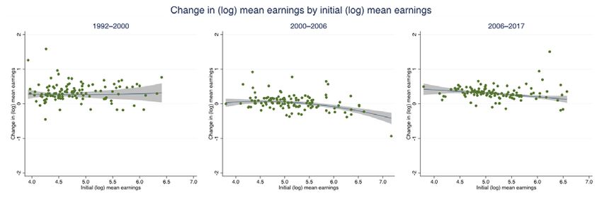
US Occupation Information Network survey (O*NET 2003); and the country-specific values of
standard task measures at the ISCO-88 two-digit level estimated for Chile by Lewandowski et al.
(2020), using information on the task content of occupations from PIAAC data, collected by the
OECD (2014/15).

Taking advantage of the trajectory that income inequality has followed in Chile, we divide the
analysis into three sub-periods: 1992–2000, 2000–06, and 2006–17. The first part of our analysis
shows that the share of the top earnings decile has been falling since 2000. In the period 2000–06,
wages grew faster around the median of the distribution, with pro-poor growth only after 2006.
The period 2006–17 describes strong growth for the bottom 30 per cent of the wage distribution
and below-average growth for the top 30 per cent. Therefore, the decrease in total inequality in
2000–06 is explained by a fall in the top decile of income distributed, more noticeably, around the
median, while the fall in total inequality in 2006–17 is related to a redistribution from the richest
30 per cent to the poorest 30 per cent.

Sectorial changes in the occupational structure confirm a displacement of workers from low-skill
occupations such as skilled agricultural, craft and trade, and elementary occupations, towards jobs
demanding non-routine higher skills, including professionals and technicians. There is also a
significant increase in the share of service and sales workers, who tend to perform routine manual
and cognitive tasks. Changes in occupational earnings have had a positive equalizing effect, with
more substantial gains in favour of lower-skill occupations such as skilled agricultural workers, craft
and related trade workers, plant and machine operators, and elementary occupations. The
equalizing effect is also noticeable at the top of the skill premium, with earnings of managers and
professionals becoming closer. Despite these positive changes to inequality, we still observe
substantial differences between the rewards of low- and high-skill occupations.

We do not find statistically significant evidence of employment or earnings polarization. The
polarization phenomenon predicts an increase in the relative demand for well-paid skilled jobs
(which consist of non-routine cognitive tasks), and low-paid low-skill jobs (linked to non-routine
manual tasks), diminishing the relative demand in the middle of the distribution, which commonly
executes routine manual and cognitive tasks. We find a significant opposite pattern (inverted U-
shaped growth) in (log) earnings in 2000–06. This suggests that real earnings grew more in the
middle of the distribution. We find that the routine task intensity (RTI) explains an important part
of the variability of earnings, and to a lesser extent, the variability of employment. There is a positive
and significant relationship between changes in mean log wage and both RTI measures (O*Net
and country-specific) in 2000–06 and 2006–17, suggesting that earnings tend to increase more in
more routine occupations, which is not observed in employment in 2006–17.

The first part of the decomposition analysis (Shapley decomposition) shows that the dispersion of
earnings is large both between and within occupations, although with a strong decline in inequality
between occupations from the 2000s. This is driven mostly by changes in average earnings, not in
shares, despite all the structural changes in employment experienced in Chile, such as increasing
average years of education, displacement of workers from low-skill occupations towards jobs
demanding non-routine higher skills, reduction of informal jobs, and increasing female
participation. Average earnings across occupations have become less unequal over time, and the
strong monotonic correlation with RTI has been reducing.

The recentred influence function (RIF) decomposition shows that both the composition and the
structure effect are important in explaining the changes in inequality in Chile, and the latter is more
relevant from 2000. In the decomposition of changes in the Gini coefficient, we observe an
inequality-enhancing effect of the returns to education and an inequality-reducing effect of the
returns to tasks in the 2006–17 period (structure effect). The composition effect is mainly driven
by changes in education (increasing schooling levels) and routinization (movements towards high-

 4

skill or less-routine occupations), and informality. When analysing the changes in the variability of
earnings by percentiles, we also observe the preponderant role of routinization and education. The
total effect of RTIs is positive throughout the entire earnings distribution and accounts for the
majority of the changes in the variability of earnings. Education is the second most relevant
covariate in explaining changes in inequality in the overall period. Since the composition and
returns effects have opposite signs, the total effect of education is inequality-reducing in the bottom
part of the distribution and inequality-enhancing in the upper part.

The remainder of the paper is structured as follows: the next section describes the data and the
conceptual framework of occupational tasks and labour market outcomes, job polarization, and
inequality decompositions. The third section describes the general trends in inequality, minimum
wage, unemployment, and informality in Chile in the period 1992–2017, analysing structural
changes in education in terms of its returns over time. In this section we also review the trend in
inequality in real earnings and occupations over time. The fourth section examines the role of tasks
and skills in changing earnings inequality over time and provides evidence to discard the hypothesis
of occupational and earnings polarization. The final empirical section analyses the role of
occupational changes in shaping the evolution of inequality by performing two inequality
decompositions, i.e. the Shapley decomposition and the RIF regression decomposition.

2 Data and methodology

This study draws on the Chilean household survey CASEN in four waves: 1992, 2000, 2006, and
2017. This is a cross-sectional household survey that uses a multi-stage stratified sampling design,
representative at the national and regional levels. The 1992 wave is the first using the ISCO-88
classification of jobs at the three-digit level, and from subsequent waves ISCO-88 at the four-digit
level is used. The CASEN survey holds a wealth of information on the demographics and income
sources of all household members aged 14 and above. This analysis focuses on a subsample of the
working-age population, this being individuals aged between 15 and 64 years active in the labour
market as employees, employers, or self-employed. Hence, unpaid family workers are excluded
from the sample.

The income concept used is labour earnings from the main occupation. This includes earnings
from dependent and independent work (cash and in kind), net of direct taxes and social security
contributions, while also incorporating income from self-production. We chose this income
concept since the occupational data are associated with the main occupation. The survey provides
net monthly earnings in Chilean pesos for each year, which have been transformed into weekly
earnings. These have been corrected to observe real earnings at November 2017 prices in
purchasing power parity (PPP) to ensure comparability over time and across countries.

Traditionally, income concepts from the survey were adjusted to match the national accounts. This
practice was removed in 2015, correcting previous waves to allow comparability. Initially they were
adjusted back to the 2006 wave, but recently all databases since 1990 have been updated. This study
uses the complementary income bases published in March 2020 by the Ministry of Social
Development, adjusted to the new methodology, which allows comparability of the income
concepts for the entire period of analysis, in our case 1992–2017.

We divide the analysis into three subperiods—1992–2000, 2000–06, and 2006–17—as well as
looking at overall change from 1992 to 2017. The selection of these particular years is based on the
trajectory that income inequality has followed in Chile. Between 1992 and 2000 the net Gini
coefficient rose slightly. From 2000 it began on a downward trajectory, with the largest drop
between 2000 and 2006. The last period, longer than the previous one, saw a milder drop in

 5

inequality, since it remained almost constant until 2012, then it fell and rose slightly between 2015
and 2017.

In order to analyse the distributional changes and task composition, this paper uses a task-based
approach, comparing the results obtained by two different methods of imputing RTI to
occupations, as in Gradín and Schotte (2020). The first method is the standard method used in the
literature that matches country survey data at the ISCO-88 three-digit level to the US estimation of
tasks derived from O*NET. The second uses country-specific values of standard task measures at
the ISCO-88 two-digit level estimated for Chile by Lewandowski et al. (2020). They construct
country-specific task measures for 46 countries, using information on the task content of
occupations from PIAAC data in the case of Chile, collected in 2014/15 by the OECD.

2.1 Occupational tasks and labour market outcomes

To identify the effect of technological change on occupations, the model developed by Autor et al.
(2003) (here after called the ALM model) shifts attention from skills (usually measured by years of
schooling) to the task contents of work. The ALM model predicts two outcomes depending on the
type of task that workers perform. First, there will be a progressive substitution of workers
performing routine tasks that are simple to codify, which can be easily replicated by machines.
Second, the ALM model predicts complementarity between technology and abstract tasks. Abstract
tasks, which require complex analytical thinking, flexibility, creativity, and communication skills,
are not only difficult to replace by machines, but they can also be complementary to computer
technologies.

Goos and Manning (2007) used the ALM model to understand the impact of technology on job
polarization. This phenomenon occurs when the relative demand for well-paid skilled jobs and
low-paid low-skilled jobs increases, diminishing the relative demand in the middle of the
distribution. While skilled jobs are characterized by the performance of non-routine cognitive tasks,
low-skilled jobs consist mostly of non-routine manual tasks. Middle-skill jobs, on the other hand,
commonly involve executing routine manual and cognitive tasks. Routine tasks that can be
displaced by technology include jobs such as manual crafting and bookkeeping, which require
precision and, hence, were never the lowest-paid occupations in the labour market. Non-routine
tasks that are complementary to technology include skilled professional and managerial jobs that
tend to be in the upper part of the wage distribution. Non-routine manual tasks that make up many
of the less-skilled jobs, such as cleaning, are not greatly affected by technology. However, the
impact of technology in other parts of the economy is likely to lead to a rise in employment in
these less-skilled jobs.

Country-specific measures of the task content of jobs have only recently become available for some
developing countries (Lewandowski et al. 2019). For that reason, most studies have relied on
standardized indices of different types of job tasks derived from the US Occupation Information
Network survey (O*NET), as in Acemoglu and Autor (2011). They associated the task measures
with common occupational categories: non-routine cognitive analytical (managerial, professional,
and technical occupations), routine cognitive (clerical, administrative, and sales occupations),
routine manual (production and operative occupations), and non-routine manual (service
occupations). The use of O*NET task data essentially relies on the assumption that the task content
of occupations is identical across countries. This assumption might be problematic particularly for
less developed countries, considering that large differences in labour productivity, technology
adoption, and skills still persist. As shown by Lewandowski et al. (2019), the task content of
occupations differs across countries, with workers in countries with higher technology use, higher
skills, and broader participation in global value chains tending to perform less-routine tasks than
their counterparts in countries with lower technology use, lower skills, and narrow specialization
in global value chains.

 6

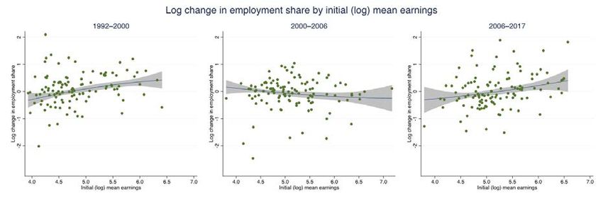
Following Autor and Dorn (2009; 2013) and Goos et al. (2014), Lewandowski et al. (2020)
construct country-specific task measures for 46 countries including Chile, using information on the
task content of occupations from the STEP, CULS, and PIAAC surveys (PIAAC in the case of
Chile).

They define a measure of relative RTI as:
 + 
 = ln� � − ln � � (1)
 2

where , , and are routine cognitive, non-routine cognitive
analytical, and non-routine cognitive personal task levels, respectively. Their definition omits
manual tasks, since the survey data do not distinguish between routine and non-routine manual
tasks and the available manual task measure is not entirely comparable across countries.
Nevertheless, the survey-based RTI measure successfully captures the routine nature of work, even
for manual jobs.

2.2 Test for job polarization

To identify the presence of job polarization, we closely follow Goos and Manning (2007) and
Sebastian (2018), who test the significance of the parameters of the following quadratic model:
 2
 ∆ log , = 0 + 1 log� , −1 � + 2 log� , −1 � (2)

where ∆ log is the change in the (log) employment share of occupation between survey wave
 − 1 and , log� , −1 � is the logarithm of the mean labour earnings in occupation in survey
 2
wave − 1, and log� , −1 � is the square of initial (log) mean labour earnings.

The same model is also estimated using (log) change in earnings as the dependent variable
(Sebastian 2018):
 2
 ∆ log� , � = 0 + 1 log� , −1 � + 2 log� , −1 � (3)
Both equations are estimated by weighting each occupation by its initial employment share to avoid
results being biased by compositional changes in small occupation groups. A polarization U-shaped
pattern implies that the first coefficient is significantly negative, with a positive quadratic
coefficient.

Following Sebastian (2018), in the next step we estimate a quadratic regression, at the three-digit
occupational level, of the log change in employment share on the initial level of routine intensity.
We aim to explain the variance of employment and earnings using our measures of the RTI of jobs.
Where measures the (time-invariant) RTI of occupation j:
 2
 ∆ log , = 0 + 1 + 2 � � (4)

 2
 ∆ log� , � = 0 + 1 + 2 � � (5)

A negative relationship between the two variables would be expected, indicating that higher RTI
leads to larger declines in employment and earnings.

 7

2.3 Shapley decomposition

Initially applied to game theory, the Shapley value (Shapley 1953, in Roth 1989) provides a
framework to decompose total inequality by factor components (Shorrocks 1982) or by subgroups
of variables (Shorrocks 2013). Intuitively, the decomposition, also known as the Shapley-Shorrocks
decomposition, allows us to estimate the partial shares of the contribution of income inequality to
changes in within-occupations inequality and between-occupations inequality.

As the Gini index is not additively decomposable, to perform the Shapley decomposition we
estimate the marginal contribution of the within- and between-occupations components of the
overall inequality following Duclos and Araar (2006). To compute the marginal contribution of
each of these factors, first we eliminate within-occupations inequality by replacing each
observation’s earnings, , with the average earnings of the occupation the person belongs to, ,
calculating between-occupations inequality. Second, we eliminate between-occupations inequality
by rescaling each worker’s earnings so that all occupations have the same average earnings, .

More formally, we want to express total inequality as:

 = + ℎ (6)

To compute the contribution of between-occupations inequality, we calculate the change in
inequality observed when the mean incomes of the occupations are equalized. Hence, the Shapley
contribution to between-occupations inequality is given by:
 1
 = [ ( ) + − ( )] (7)
 2

Similarly, the Shapley contribution of within-occupations inequality is given by:
 1
 ℎ = [ ( ) + − ( )] (8)
 2

Therefore, changes in the Gini index can be decomposed into the contribution of each component.

We repeat the analysis with counterfactual distributions in which either the occupational shares or
the occupational earnings are kept constant, to check whether the trend is explained by changes in
the distributions of employment or changes in earnings.

2.4 Concentration index

We use the concentration index derived from the concentration curve that is commonly used to
analyse inequalities in health (Wagstaff et al. 1991) to investigate the relevance of the task
composition of occupations in explaining trends in inequality between occupations. The
concentration curve shows the share of the population that receives a proportion of the earnings
when we order the population from highest to lowest RTI content of jobs, instead of by earnings
as in the Lorenz curve. If RTI is equally distributed across occupations, the concentration curve
will coincide with the diagonal; if high-routine jobs are concentrated among the worst-paid
occupations, the concentration curve lies below the diagonal. The further the curve lies below the
diagonal, the higher the degree of inequality related to the routine-task contents of jobs.

The concentration index denoted by C is defined as twice the area between the concentration curve
and the diagonal. The concentration index is positive when the concentration curve lies below the
diagonal and negative when it lies above the diagonal. Thus, the lowest value that C can take is –1,
when all routine tasks are done by the most disadvantaged person (so that C is shaped as follows: ).

 8

The maximum value the index can take is +1, when all routine tasks are concentrated in the hands
of the richest person (so that C is shaped as follows: ). C corresponds to the Gini index when RTI
is perfectly correlated to average earnings. Therefore, the closer the value of the concentration
index is to the Gini index, the higher the correlation between RTI and earnings.

2.5 RIF regression decomposition

Developed by Firpo et al. (2011, 2018), recentred influence function (RIF) regression is an
extension of the Oaxaca-Blinder (OB) decomposition (Blinder 1973; Oaxaca 1973). The OB
procedure provides a way of decomposing differences in mean earnings into a composition effect
(changes due to varying worker characteristics) and a structure effect (changes in the return to those
characteristics). It also allows us to further divide these two components into the contribution of
each covariate. The main advantage of using the RIF regression method in an OB-type
decomposition is that it provides a linear approximation of highly non-linear functionals, such as
the quantiles or the Gini coefficient (Firpo et al. 2018).

The RIF method is a two-stage procedure that can be used to perform OB-type decompositions
on any distributional measure, not only the mean. The first stage consists of decomposing the
distributional statistic of interest (i.e. interquartile ranges and the Gini coefficient) into an earnings
structure and a composition component using a reweighting approach, where the weights are either
parametrically or non-parametrically estimated. In a second stage, the wage structure and
composition effects are further divided into the contribution of each covariate, as in the usual OB
decomposition (Firpo et al. 2018).

Closely following Firpo et al. (2011), we focus on differences in the wage distributions, ∆ , , for
two time periods, 1 and 0:

 ∆ = � 1 | =1 � − � 0 | =0 � (9)

where � 0 | =0 � is the wage distribution in time period 0, and � 1 | =1 � is the wage distribution
in time period 1. Adding and subtracting the term � 0 | =1 �, we obtain:

 ∆ = � 1 | =1 � − � 0 | =1 � + � 0 | =1 � − � 0 | =0 � (10)
 ∆ ∆ 
where ∆ is the wage structure effect, ∆ is the composition effect, and � 0 | =1 � is the
counterfactual distribution that would have prevailed if workers observed in the end period
( = 1) had been paid under the wage structure of period 0.

The composition effect ∆ consists of changing the distribution of (characteristics) from its
value at = 0 to its value at = 1, holding the wage structure constant. The wage structure effect
∆ measures changes in the return to those characteristics, holding the distributions of constant.

Following DiNardo et al. (1996), Firpo et al. (2011) estimate the counterfactual distribution
 � 0 | =1 � by reweighting the period 0 data to have the same distribution of covariates as in
period 1. Details of the estimation procedure can be found in Firpo et al. (2011; 2018), Fortin et
al. (2011), and the Methodological Appendix of Gradín and Schotte (2020).

 9

3 Inequality and employment trends

3.1 Country context and inequality trends

Chile has frequently been described as a successful case of rapid economic growth, sound economic
management, macroeconomic stability, export orientation, and bold structural reforms, such as
trade and foreign investment liberalization. Most of these pro-market reforms were implemented
during the military dictatorship in the 1980s. They also included a bundle of social reforms in the
areas of education, health, and pensions that aimed to increase the private sector role in the
provision of these services.

Market-oriented reforms boosted the economy strongly during the 1990s, allowing average growth
rates of more than 7 per cent between 1991 and 1998 (Figure A1 in the Appendix). The return to
democracy was a period of rising private investment and job creation that helped to reverse the
rises in unemployment and depression of real wages of the dictatorship period in the 1980s
(Contreras and Ffrench-Davis 2012). The rapid growth moved Chile from having the third-lowest
GDP per capita in South America, US$4,511, in 1990 to taking the lead in the region from 2010,
reaching $25,155 in 2019 (Figure A2 in the Appendix).

High growth had a positive effect, facilitating the reduction of poverty from almost 40 per cent in
1990 to 20.2 per cent in 2000 (Contreras 2003). After 2000 the poverty rate reduced further,
reaching 8.7 per cent in 2017 (MDS and PNUD 2020). 1 This was accompanied by increased social
spending and the creation of a social protection system, which has played a key role in overcoming
extreme poverty and improving the quality of life of the most deprived in the last few decades.

Despite the good economic results and poverty reduction, other social indicators have not had
such a satisfactory evolution. Chile exhibits persistent inequality of income and wealth, with high
asset concentration among powerful economic elites. The Gini coefficient for both monetary
incomes (adjusting for transfers) and net wealth places Chile as the most unequal country in the
OECD, and it ranks 28th among the countries with the highest inequality in the world, preceded
only by other countries in Latin America and Sub-Saharan Africa (OECD 2020; World Bank
2020c).

An important cause of the inequality in Chile is the large income gap between the elite and the rest
of the population. In 2017, the richest 1 per cent captured 27.8 per cent of national income; at the
same time, the income share of the wealthiest 10 per cent was 60.2 per cent (survey and tax data;
WID 2020). Additionally, the wealthiest 10 per cent’s share of autonomous income was 30.8 times
higher than the share of the poorest decile (survey data only). Considering job earnings, this ratio
increases to 39.1 (MDS and PNUD 2020). When considering monetary household income, this
gap is reduced due to transfers and state subsidies, which have increased since the 1990s. However,
analysing the redistributive power of these social policies, we observe that this is rather limited and
much lower than that of other OECD countries. Before taxes and transfers, income inequality in
Chile is similar to that of countries such as Belgium and Austria and even lower than that of
Finland, France, and Ireland (OECD 2020). The big difference is the redistributive capacity of the
state, which in Chile is minimal, leaving the country the most unequal of all the OECD members.

1
 This poverty line is calculated using the ‘historical methodology’ applied by the Economic Commission for Latin
America and the Caribbean, ECLAC (MDS and PNUD 2020), which estimates the poverty threshold from the basic
food basket (BFB) based on the IV Family Budget Survey 1987–88 (EPF). This value is updated over time according
to the variation in the price of each of the elements in the BFB. As a welfare indicator, it uses total per capita household
income corrected for non-response and adjusted to match the national accounts.

 10

Social reforms implemented since the 1980s were promoted as a way to improve efficiency and
increase individual choice. However, the segmentation in health, education, and social security
benefits has fostered profound inequalities in access to quality services which, combined, enhance
inequalities in other areas of life. For example, limited access to quality education for the poorest
translates into unequal opportunities in the labour market, which also influences participation in
the health system and limits contributions to the pension scheme. Unequal access to opportunities,
a greater demand for quality public services, and the high level of indebtedness of Chilean families
has formed great social tensions for more than a decade, which erupted in the outbreak of social
unrest of October 2019. This social unrest has been positively led towards a process of
constitutional change that began at the end of October 2020, when a public vote approved
changing the constitution implemented during the dictatorship. The new constitution is seen as a
step towards a new social contract in Chile.

Although inequality in Chile is high, it has been declining slightly since the turn of the century, as
shown in Figure 1. While most of the developed world experienced rising inequality in the 2000s,
Chile and many countries in Latin America followed the opposite pattern. In Chile the Gini
coefficient of earnings fell from 0.546 in 2000 to 0.501 in 2017, with the largest drop of 0.035
points between 2000 and 2006. The literature mentions as the main causes of this inequality drop
the reduction in the wage gap between the highest- and lowest-skilled workers due to faster growth
of real wages at the bottom of the wage distribution than at the top, improvements in the minimum
wage, a lower skill premium, and better-targeted cash transfers to the poor, combined with a
positive economic environment and the commodity price boom (Messina and Silva 2019; PNUD
2017; Torche 2014).
Figure 1: Gini of households’ earnings, Chile, 1990–2017

Note: the income series used in this graph have recently been adjusted by the Ministerio de Desarrollo Social
(MDS) to the new methodology, to allow the comparison of inequality measures since the 1990s.
Source: author’s illustration based on data from MDS and PNUD (2020).

3.2 Labour market institutional factors that affect inequality

The Chilean labour market is characterized by low wages. In 2018, 57 per cent of those employed
did not earn enough to lift an average family out of poverty. 2 In the case of female heads of
households, this percentage was 64 per cent. Additionally, 51 per cent of private sector workers

2
 This is based on the monthly income poverty line for an average household of four people, which in November 2018
was 430,763 Chilean pesos, equivalent to US$621.

 11

with full-time jobs, were in the same situation, revealing high levels of precariousness in the job
market (Kremerman and Durán 2019).

In addition to low incomes, the precariousness of the Chilean labour market has various other
origins, including excessive dependence on self-employment and short-term contracts. The share
of temporary contracts, although it has decreased since 2012, is the second-highest among OECD
countries (27 per cent). The level of informality, or the proportion of wage earners and self-
employed workers not making contributions to the pension system, is also one of the highest in
the OECD, standing at 32 per cent of employment in 2015, held back only by cyclical conditions
(OECD 2018). Informality particularly affects lower-skilled workers, young people, immigrants,
indigenous people, and women. Between 2017 and 2019, women had informality rates almost three
percentage points higher than those of men (INE 2017). Temporary and informal workers
generally face lower wages and frequent periods of unemployment and inactivity. Given that Chile
has a private pension system based mainly on individual savings, high levels of informality puts
pressure on the pension scheme. This is why the pension law established voluntary contributions
for self-employed workers in 2014; these have been compulsory only since 2018 (SII 2020).

Chilean labour market regulations may seem rigid de facto, but in practice it is quite easy for
companies to hire and fire workers. The type of employment contract—permanent or temporary—
is a fundamental distinguishing characteristic that creates a segmented or dual market, where
temporary contracts are generally associated with flexibility and permanent contracts with rigidity
(Ruiz-Tagle and Sehnbruch 2015). In 2014, 51 per cent of workers in the formal sector had
contracts of less than three years, mainly in the services sector—the sector with the highest level
of job creation in the last two decades. In addition, a third of workers had short-term fixed
contracts, used largely in construction and agriculture (Dirección del Trabajo 2014); the OECD
average for these types of contracts is 12 per cent (OECD 2016). While in more developed
countries a short-term contract can be the path to a permanent job, in Chile 40.9 per cent of these
contracts are renewed as short-term after their expiration, and only 36.8 per cent lead to permanent
jobs (Dirección del Trabajo 2014, cited in PNUD 2017). Another factor that affects job stability is
outsourcing; this is a common practice in Chile that in 2014 affected 17 per cent of the workforce
(Dirección del Trabajo 2014).

These practices limit the real labour rights of employees, preventing their access to severance pay,
the possibility of creating effective unions, and access to benefits such as nurseries. Other aspects
of labour market flexibility include low unionization rates, limited strike rights (replacement of
striking workers is allowed), decentralized and fragmented bargaining power, and highly flexible
lay-off laws for workers on permanent contracts (OECD 2018).

The short duration of contracts and high job turnover also limits the coverage and benefits of
unemployment insurance—which is financed with contributions from the employee and the
employer. Only 50 per cent of those whose contracts end in a year have enough contributions in
their accounts to access unemployment insurance. In 2015, 50 per cent of workers with a fixed-
term contract had gaps in their contributions of more than three months, which prevents them
from accessing the public unemployment fund (Fondo de Cesantía Solidario) (Sehnbruch et al.
2019). All of this ‘flexibility’ in the Chilean labour market transfers the risks from the employer
(and the state) to the employee, leaving workers more vulnerable to possible external shocks and
increasing inequality as there are no adequate safety nets for them (World Bank 2017).

 12

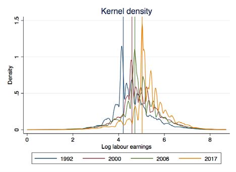
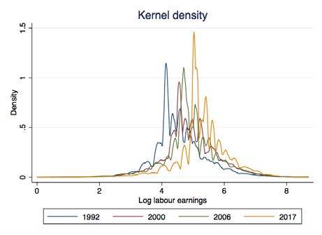
Figure 2: Weekly minimum wage, Chile

 180
 160
 CL pesos of 2017 in PPP

 140
 120
 100
 80
 60
 40
 20
 0
 1992
 1993
 1994
 1995
 1996
 1997
 1998
 1999
 2000
 2001
 2002
 2003
 2004
 2005
 2006
 2007
 2008
 2009
 2010
 2011
 2012
 2013
 2014
 2015
 2016
 2017
Note: the Chilean Congress adjusts nominal minimum wage annually; in all tables and figures in this paper,
monthly values in Chilean pesos for each year have been converted into weekly values in 2017 pesos and then
adjusted by purchasing power parity.
Source: author’s illustration based on annual changes to the minimum wage law published by Congreso de Chile.

Figure 3: Kernel density functions

 (a) (b)

Source: authors’ elaboration based on CASEN (1992, 2000, 2006, 2017).

Sustained increases in the minimum wage have been mentioned as a preponderant factor in the
reduction of inequality. The real minimum wage increased at an average annual rate of 4 per cent
during the 1990s, reducing to an average of 3 per cent annually during the 2000s (Figure 2). Kernel
densities (Figure 3, graph b) show the effect of the minimum wage on the earnings distribution.
Vertical lines indicate the minimum wages of each year, which coincide with the jumps in the
density function. We observe increases in the minimum wage as movements of the vertical lines to
the right, and a flattening of the density functions below the minimum wage over time. The
percentage of the population with earnings below the minimum wage first increases from 35 to 37
per cent between 1992 and 2000, which coincides with the largest jump in the minimum wage
(Figure 2). From 2000, the population below the minimum wage dropped to 33 per cent in 2006
and to 31 per cent in 2017.

 13

3.3 Skill supply and premium

Education impacts earnings through diverse channels. It affects labour participation at different
stages of the life cycle, as well as the amounts of time worked, and the frequency and duration of
unemployment and part-time employment, among other factors (INE 2017). Chile, like the rest of
Latin America, has been characterized by high returns to secondary and tertiary education (notably
higher education in the case of Chile). This high school premium has been the result of educational
policies that focused on increasing the coverage of tertiary education before expanding secondary
schooling: 3 a very different strategy compared with Asian countries, which prioritized eliminating
the bottom tail of the educational distribution by universalizing secondary education (Morley 2001).
The result is a heavily polarized distribution of educational attainment, which gives a historically
significant premium to those with secondary and post-secondary education (Torche 2014).

Average years of education have risen rapidly, from 12.9 in 1990 to 16.5 in 2018, due to a large
structural expansion that increased school coverage since the 1980s and access to higher education
since the 1990s (UNDP 2019). Figure 4 displays the level of educational attainment of the adult
population aged between 15 and 64 at the time of observation. We differentiate between four
completed levels of education: no formal education, completed primary, completed secondary, and
completed tertiary. Although a significant share of the population still has low levels of education
(8 per cent in 2017), the expansion at all levels has been pronounced.
Figure 4: Distribution of workers by level of education

Source: author’s illustration based on CASEN (1992, 2000, 2006, 2017).

The increase in schooling has been reflected in real wages, which have grown at all educational
levels. Figure 5 displays average weekly earnings (primary occupation) across different schooling
levels. This is a cross-section of the population at one point in time rather than an analysis of
individual lifetime earnings; it tells us how much workers earn according to the level of education
they have attained (Table A1 in the Appendix).

3
 Secondary education in Chile has been compulsory since 2003 (Law No. 19,876) and the expansion of university
education began with the educational reform of 1981, increasing more strongly since 1990 with the return to democracy
in the country (Gaentzsch and Zapata-Román 2020).

 14

We observe that returns to tertiary education in Chile are very high: earnings of higher education
graduates by far exceed those of all other levels. These differences are accentuated by gender
differences. The salary of men with a higher education degree in 1992 was 6.2 times higher than
that of their peers without formal education, while that of women at the same level was only 3.6
times higher (Table A2 in the Appendix). We notice that polarization of educational returns has
decreased since 2000: the earnings ratio between people holding a university degree and those
having no formal education (or primary incomplete) has moved from 4.9 in 1992 to 5.8 in 2000,
decreasing to 4.5 and 3.5 in 2006 and 2017 respectively.

Returns to education have grown differently for different groups in the periods analysed. From
1992 to 2000, we observe higher school premium growth as the educational level increases
(Figure A2 in the Appendix): the average annual growth rate of the salaries of workers with no
formal education was 1.9 per cent, while that of people with primary, secondary, and tertiary
education was 2.1, 2.7, and 3.9 per cent respectively. In the period 2000 to 2006, we observe the
opposite pattern: the wages that grew the most were those of less-qualified workers, at an average
annual rate of 2.2 per cent, while the salary increase for workers with primary education was 1.2
per cent per year, and a negative annual growth rate of −1.9 and −2.0 is observed for the groups
with secondary and tertiary education. A similar development is observed from 2013 to 2017:
smaller premiums as the educational level increases, but not negative growth for the most skilled
workers.
Figure 5: Mean weekly real earnings by level of education

 800

 600

 400

 200

 0
 None Primary Secondary Tertiary None Primary Secondary Tertiary None Primary Secondary Tertiary
 Total Male Female

 1992 2000 2006 2017

Source: author’s illustration based on CASEN (1992, 2000, 2006, 2017).

When controlling for age, macro region of residence, having a formal job, and occupations at two-
digit level for both men and women, we confirm sizeable gender differences (Figure 6): returns to
education are always lower for women. We observe that average school premiums increased for
men from 1992 to 2000, at every level of education, except for the most skilled workers, for whom
the premium remains almost unchanged in the period. For women, returns to secondary and
tertiary education increase in the period, but they decrease slightly for those with primary education.
Between 2000 and 2006, educational premiums decrease slightly, except for women with primary
education. After 2006, there is a more pronounced reduction in the returns to education in general
for both men and women, but it is more so for those holding a higher education degree. Even
though returns to tertiary education decreased, particularly for men, they are still very high
compared with those for lower levels of education. 4

4
 The large skill premium of higher education in Chile is mainly driven by university graduates who come from a
background of having highly educated parents. As suggested by the theory of inequality of opportunity, parental

 15

Undoubtedly, these falls in the returns to education have contributed strongly to the reduction of
inequality in Chile. However, this analysis does not allow us to establish whether or not changes in
returns to education are the main source of wage inequality in Chile, as mentioned in the literature
(PNUD 2017; Torche 2014). We expect to complement this analysis and provide further insights
into the relevance of educational premiums to inequality movements in the decomposition section.
Figure 6: Changes in the education premium on log labour earnings

 1 1
 Education premium on log earnings

 Education premium on log earnings
 0.8 0.8

 0.6 0.6
 Tertiary
 Secondary
 0.4 0.4
 Primary
 No schooling
 0.2 0.2

 0 0
 1992 2000 2006 2017 1992 2000 2006 2017
 Male Female

Note: log weekly earnings are regressed in each year separately by gender, dummy variables for three education
levels (tertiary, secondary, primary, with no schooling as the base category), two age groups (ages 15–24 and
45–64, with 25–44 as the base category), three regional dummies (north, centre, and capital, with south as the
base category), occupations at the ISCO-88 two-digit level, and a dummy variable for formality in the job market.
The figure shows the coefficient estimates on the educational categories, which directly measure the returns to
attaining a higher level of education in terms of (log) weekly earnings across survey waves, separately by
gender.
Source: author’s illustration based on CASEN (1992, 2000, 2006, 2017).

4 Earnings inequality

4.1 Trend in inequality in real earnings over time

As mentioned in the previous section, a significant source of inequality in Chile is high income
shares at the top of the distribution. Analysing the data from the income survey CASEN, in 2017
the wealthier decile appropriated 36.5 per cent of total earnings, while the most deprived decile
only got 1.7 per cent, as shown in Figure 7. In other words, the richest decile had 21 times the
earnings of the poorest decile in 2017. Although the share of the bottom decile did not increase
significantly between 2000 and 2006, that of the wealthiest decile decreased by 3.7 percentage
points. Between 2006 and 2017, the top share fell a further 2.5 percentage points. It is interesting
to notice that the major gains in both periods after the 2000s were below the median of the
distribution.

education often intersects with other forms of advantage such as financial and social capital, which help graduates with
more-advantaged family backgrounds to secure better-paid jobs (Gaentzsch and Zapata-Román 2020).

 16

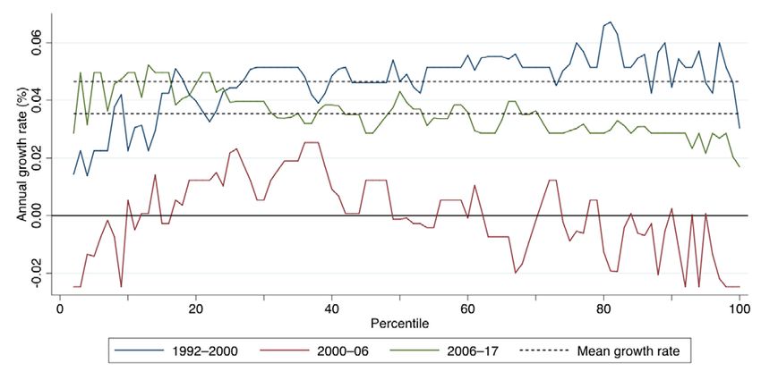
Figure 7: Decile shares and variations (weekly log real earnings)

Source: author’s illustration based on CASEN (1992, 2000, 2006, 2017).

Summary inequality indices and inter-quantile ratios in Table 1, as well as the growth incidence
curves (GIC) in Figure 8, complement the preceding analysis. Table 1 shows, on the left-hand side,
the evolution of three inequality indices for the whole earnings distribution. We observe the rise
previously described in the period 1992–2000, and subsequent falls after 2000. Inter-quantile ratios
on the right-hand side of the table show differences at three points of the distribution. The gap
between the 90th and the 10th percentile shows the income level of individuals in the top 10 per
cent of the income distribution relative to those of individuals in the bottom 10 per cent. The 90–
10 ratio confirms a gain for the wealthiest decile relative to the poorest in the first period (1992–
2000), followed by relative losses for the top decile in subsequent periods. The 90–50 ratio shows
the gap between the 90th percentile and the median, which also increases in the first period and
shrinks thereafter. The 50–10 ratio illustrates the gap between the median and the 10th percentile,
which, interestingly, increased until 2006 and only slightly declined after 2006—suggesting larger
gains for the middle of the distribution between 2000 and 2006 and pro-poor growth only after
2006.
Table 1: Summary inequality indices and Inter-quantile ratios

Summary indices Inter-quantile ratios
 1992 2000 2006 2017 1992 2000 2006 2017
Var (log earn) 0.718 0.806 0.761 0.658 ln(q90)–ln(q10) 1.974 2.157 2.120 1.897
Gini (log earn) 0.099 0.098 0.094 0.081 ln(q90)–ln(q50) 1.186 1.226 1.165 1.050
Gini (earn) 0.504 0.514 0.475 0.443 ln(q50)–ln(q10) 0.789 0.931 0.956 0.847

Source: author’s construction based on CASEN (1992, 2000, 2006, 2017).

The GIC (Figure 8) indicates the growth rate in income between two points in time at each
percentile of the distribution. Between 1992 and 2000 (blue line), real earnings grew along the
whole distribution. However, we observe some redistribution from those below the median
(growth rates mainly below the average marked by the top dotted line) to those above the median
(growth rates mainly above the average). In the second period, 2000–06 (red line), we observe
negative growth—also below the median—for the top quintile (from the 80th percentile), as well
as for the bottom decile, and positive and above-average growth mainly from the 20th percentile
to the median. This is very different from the growth pattern of the last period (2006–17), for

 17

which we observe strong growth for the bottom 30 per cent and below-average growth for the top
30 per cent. This last trend at the extremes of the distribution would have been inequality-reducing.
Figure 8: Growth incidence curves

Source: author’s illustration based on CASEN (1992, 2000, 2006, 2017).

4.2 Structural changes in employment

Structural transformations in the Chilean productive structure in the last 50 years have had a strong
impact on the country's employment structure in the present. We observe a reduction in the shares
of agriculture and the manufacturing sector, along with the growth of the services and financial
sectors, as well as the mining sector. Services tend to be labour-intensive but not technology-
intensive; and mining is technology-intensive but requires few workers, most of whom are highly
qualified (Solimano and Zapata-Román 2019). Table 2 shows the large decline in the share of
agricultural employment, which in 1992 accounted for almost 16 per cent of total jobs but in 2017
had declined to 9 per cent. A similar development was experienced by the manufacturing sector,
which in 1992 had almost 18 per cent of the workforce, falling to less than 10 per cent in 2017.
The services sector absorbed the decrease in employment in agriculture, mining, and
manufacturing, becoming the largest sector by employment, with 70 per cent of the total workforce
and 86 per cent of female workers, in 2017.

Real wages grew between 1992 and 2000 in all sectors for men and women, except for women
employed in industries that comprised electricity, gas, water supply, and construction—and this
represented only 1.3 per cent of the female workforce (Table 3). We observe the opposite
development in 2000–06, with real earnings decreasing on average, particularly in mining, which
had had the largest rise in the previous period. In the last period (2006–17), we observe positive
and similar growth rates between sectors. Summarizing, we find that the first period of growing
inequality is associated with an increase in wages in all economic sectors. The second period (the
shortest), with the most substantial decrease in inequality, is associated with a reduction in real
wages, particularly in the better-paid industries. Finally, the most recent period was one of
decreasing inequality but in which wages grew more homogeneously in all sectors.

 18

Table 2: Distribution of workers by industry and gender

 All Male Female

 1992 2000 2006 2017 1992 2000 2006 2017 1992 2000 2006 2017

Agriculture (A+B) 15.77 12.73 12.39 8.99 20.48 17.12 15.91 11.65 6.28 5.29 6.88 5.66

Mining (C) 2.21 1.60 1.75 1.85 3.14 2.40 2.71 2.99 0.35 0.25 0.26 0.41

Manufacturing (D) 17.09 14.11 13.82 9.38 17.82 15.99 15.84 11.84 15.62 10.92 10.65 6.31

Other industries (E+F) 9.79 9.18 10.08 9.86 14.07 13.83 15.61 16.42 1.15 1.31 1.43 1.64

Services (G−Q) 55.13 62.37 61.95 69.92 44.50 50.65 49.93 57.10 76.59 82.23 80.78 85.97

Source: author’s construction based on CASEN (1992, 2000, 2006, 2017).

Table 3: Average weekly earnings by sectors and gender

 Male Female

 Mean weekly earnings Annual growth rate Mean weekly earnings Annual growth rate

Sector 1992 2000 2006 2017 1992– 2000–06 2006–17 1992 2000 2006 2017 1992– 2000–06 2006–17
 2000 2000

Agriculture (A+B) 94 145 136 197 5.57 −1.06 3.43 80 101 114 157 2.96 2.04 2.95

Mining (C) 252 457 368 475 7.72 −3.55 2.35 211 576 400 466 13.38 −5.90 1.40

Manufacturing (D) 174 269 226 288 5.60 −2.86 2.23 115 164 143 206 4.54 −2.26 3.37

Other industries (E+F) 178 203 206 287 1.66 0.24 3.06 271 228 267 343 −2.14 2.67 2.30

Services (G−Q) 188 282 260 360 5.20 −1.34 3.00 120 181 181 256 5.27 0.00 3.20

Source: author’s construction based on CASEN (1992, 2000, 2006, 2017).

 19

4.3 Trend in occupations

In 1992, 60 per cent of the workforce in Chile was concentrated in elementary occupations, craft
and trade work, and sales (Figure 9). The share of workers in other intermediate occupations was
around 7–8 per cent, while the share in occupations associated with higher skill levels (managers
and professionals) varied between 5 and 7 per cent. In the period 1992–2000, only the participation
in elementary and trade occupations decreased, by six and four percentage points respectively. The
main growths were registered in both professional and technician occupations, where the share
increased by 2.5 percentage points, coinciding with the expansion of higher education. A low level
of growth was observed in the share of sales workers and almost no growth in the share of skilled
agriculture. The period 2000–06 registers a fall in the share of managers, clerical workers, and
skilled agriculture. Only the share of medium- and other low-skill occupations increased. In 2006–
17, the share of high-skill occupations (managers, professionals, and technicians) and sales
increased, and the share of lower-skill occupations decreased.

These sectorial changes in the occupational structure imply a displacement of workers from low-
skill occupations such as skilled agricultural, craft and trade, and elementary occupations, 5 towards
jobs demanding non-routine higher skills, including professionals and technicians. There is also a
significant increase in the share of services and sales workers, who tend to perform routine manual
and cognitive tasks. Additionally, there is a net drop in the share of managers, which is redistributed
among other professionals (at the same skill level).
Figure 9: Employment shares and changes by occupation

Note: ppts = percentage points.
Source: author’s illustration based on CASEN (1992, 2000, 2006, 2017).

When examining earnings across occupations (Figure 10), we observe large differences in returns
in favour of high-skill occupations. The earnings ratio between people in managerial positions and
those in elementary occupations was 7 in 1992, while the ratio between professionals and
elementary occupations was 5. Earnings concentration at the top was so marked in 1992 that those
employed as technicians and as clerks, who on average have a similar level of education to managers
(Figure A5 in the Appendix), had an income equivalent to half and one-third of that of managers

5
 These occupations are those with the lowest average years of education; see Figure A5 in the Appendix.
 20