Coastal submesoscale processes and their effect on phytoplankton distribution in the southeastern Bay of Biscay - Ocean Science
←
→
Page content transcription
If your browser does not render page correctly, please read the page content below

Ocean Sci., 17, 849–870, 2021
https://doi.org/10.5194/os-17-849-2021
© Author(s) 2021. This work is distributed under
the Creative Commons Attribution 4.0 License.

Coastal submesoscale processes and their effect on phytoplankton
distribution in the southeastern Bay of Biscay
Xabier Davila1,4 , Anna Rubio1 , Luis Felipe Artigas2 , Ingrid Puillat3 , Ivan Manso-Narvarte1 , Pascal Lazure3 , and
Ainhoa Caballero1
1 AZTI Marine Research, Basque Research and Technology Alliance (BRTA), Herrera Kaia,
Portualdea z/g, 20110 Pasaia, Spain
2 Université du Littoral Côte d’Opale, Université de Lille, CNRS UMR 8187 LOG, 32 Avenue Foch, 62930 Wimereux, France
3 IFREMER/Dyneco/Physed, BP 70, 29280 Plouzané, France
4 Geophysical Institute, University of Bergen and Bjerknes Centre for Climate Research, 5007 Bergen, Norway

Correspondence: Xabier Davila (xabier.davila@uib.no)

Received: 2 June 2020 – Discussion started: 18 June 2020
Revised: 27 January 2021 – Accepted: 19 May 2021 – Published: 1 July 2021

Abstract. Submesoscale processes have a determinant role           below the pycnocline and at the deep chlorophyll maximum
in the dynamics of oceans by transporting momentum, heat,          (DCM) by performing a set of generalized additive models
mass, and particles. Furthermore, they can define niches           (GAMs). Overall, salinity is the most important parameter
where different phytoplankton species flourish and accumu-         modulating not only total chl a but also the contribution of
late not only by nutrient provisioning but also by modifying       the two dominant spectral groups of phytoplankton, brown
the water column structure or active gathering through advec-      and green algae groups. However, at the DCM, among the
tion. In coastal areas, however, submesoscale oceanic pro-         measured variables, vorticity is the main modulating envi-
cesses act together with coastal ones, and their effect on phy-    ronmental factor for phytoplankton distribution and explains
toplankton distribution is not straightforward. The present        19.30 % of the variance. Since the observed distribution of
study brings the relevance of hydrodynamic variables, such         chl a within the DCM cannot be statistically explained with-
as vorticity, into consideration in the study of phytoplankton     out the vorticity, this research sheds light on the impact of
distribution, via the analysis of in situ and remote multidisci-   the dynamic variables in the distribution of spectral groups
plinary data. In situ data were obtained during the ETOILE         at high spatial resolution.
oceanographic cruise, which surveyed the Capbreton Canyon
area in the southeastern part of the Bay of Biscay in early Au-
gust 2017. The main objective of this cruise was to describe
the link between the occurrence and distribution of phy-           1   Introduction
toplankton spectral groups and mesoscale to submesoscale
ocean processes. In situ discrete hydrographic measurements        The monitoring and characterization of submesoscale dy-
and multi-spectral chlorophyll a (chl a) fluorescence profiles     namics are determinant for the appropriate comprehension
were obtained in selected stations, while temperature, con-        of marine ecosystems (Lévy et al., 2012). Submesoscale pro-
ductivity, and in vivo chl a fluorescence were also continu-       cesses refer to those features that range on spatio-temporal
ously recorded at the surface. On top of these data, remote        scales of the order of 0.1–10 km and 0.1–10 d. The timescales
sensing data available for this area, such as high-frequency       at which these processes evolve make them uniquely impor-
radar and satellite data, were also processed and analysed.        tant to the structure and functioning of planktonic ecosys-
From the joint analysis of these observations, we discuss the      tems (Lévy et al., 2012; Mahadevan, 2016). They influence
relative importance and effects of several environmental fac-      the ecosystem by either driving episodic nutrient pulses to
tors on phytoplankton spectral group distribution above and        the sunlit surface, affecting the mean time that photosynthetic
                                                                   organisms remain in the well-lit surface (Lévy et al., 2012),

Published by Copernicus Publications on behalf of the European Geosciences Union.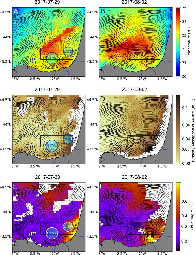
850                                         X. Davila et al.: Coastal mesoscale processes and their effect on phytoplankton

or reducing and even suppressing the biological production        of Slope Water Oceanic eDDIES (SWODDIES) (Caballero
(Gruber et al., 2011). In addition, since primary production      et al., 2016; Teles-Machado et al., 2016). Besides, the ocean
drives the absorption of atmospheric CO2 , submesoscale pro-      surface layer in this region is subjected to the seasonal vari-
cesses might actively contribute to the carbon export and         ations of the water runoff from the main nearby rivers: the
regulate the fate of particulate organic carbon (Mahadevan,       Gironde, Loire, and Adour rivers (Reverdin et al., 2013). The
2014). The effect of submesoscale processes on phytoplank-        river runoff significantly modifies the water mass adjacent to
ton also has implications for regional biogeochemical bud-        the shelf by creating turbid and diluted plumes (Ferrer et al.,
gets, plankton monitoring strategies, fisheries, and manage-      2009), which act as a nutrient source to the surface layers
ment (Irigoien et al., 2007).                                     and sustain primary production in the region (Morozov et al.,
   The influence of ocean dynamics on phytoplankton cov-          2013).
ers a wide range of spatio-temporal scales, and these are            These complex ocean dynamics can modulate phytoplank-
inherent to the surveying strategy being selected. D’Ovidio       ton occurrence in the BoB. The flow of the IPC generates a
et al. (2010) linked the occurrence of different phytoplank-      shelf-break convergent front that separates the advected high-
ton groups with the large-scale surface ocean dynamics based      salinity and warm waters from the cold fresher coastal wa-
on altimetry data. They defined the so-called fluid dynamical     ters. The vertical mixing associated with this frontal system
niches where the phytoplankton assemblages occur within           has a substantial influence on the whole plankton commu-
distinct physicochemical environments. However, available         nity (Fernández et al., 1993). Caballero et al. (2016) reported
satellite observations lack the spatio-temporal resolution to     a DCM in the centre of a SWODDY resulting from the verti-
properly resolve the fast-evolving submesoscale coastal pro-      cal velocities and eddy-wind-induced Ekman pumping in the
cesses. In coastal regions, where oceanic currents meet the       centre of the anticyclone. More recently, Muñiz et al. (2019)
sea floor, the connection between the submesoscale pro-           described the phytoplankton annual cycle in the SE-BoB and
cesses and phytoplankton becomes even more challenging            reported that temperature and nutrients explained most of the
and therefore requires more demanding surveying methods           of the variability of chl a concentration. Nevertheless, to our
that can provide a high spatio-temporal resolution. Nowa-         knowledge, none of these studies have focused on the rela-
days, autonomous gliders can typically cover 1 km horizon-        tive importance of submesoscale dynamics while analysing
tally in an hour, but even this can be too slow for synop-        hydrographic and hydrodynamic forcing mechanisms at the
tic measurements of larger submesoscale features (on scales       same time.
of 10 km). An alternative is the use of ship-towed undulat-          In order to shed light on the coastal submesoscale dy-
ing devices, which allow sampling 10–20 times faster than a       namics and their effects on chl a and phytoplankton groups
glider (Lévy et al., 2012). Regarding phytoplankton distribu-     distribution, the ETOILE oceanographic cruise surveyed the
tion, submesoscale to microscale vertical patterns of chloro-     Capbreton Canyon area in early August 2017. This cruise
phyll a (chl a) concentrations have been studied widely by        was one of the research actions in the framework of the
the use of in vivo fluorometric casts, allowing the identifi-     European H2020 Joint European Research Infrastructure
cation of the deep chlorophyll maximum (DCM) (Cullen,             for Coastal Observatory – Novel European eXpertise for
2015). Differences within the DCM in terms of concentra-          coastal observaTories (JERICO-NEXT) project. The regional
tion, biomass, and diversity stress the importance of the envi-   coastal observatories (EuskOOS) are also embedded in the
ronmental drivers involved (Latasa et al., 2017), upon which      JERICO Research Infrastructure and provide the operational
the occurrence of (sub)mesoscale processes play a critical        high-frequency (HF) radar data complementing the ETOILE
role (Lévy et al., 2012).                                         in situ measurements. JERICO-NEXT (2014–2019), its pre-
   This study focuses on the innermost southeastern region        decessor JERICO (2007–2013), and the ongoing JERICO-S3
of the Bay of Biscay (SE-BoB), a semi-open bay delim-             (2020–2024) all aim to consolidate a pan-European coastal
ited by the Spanish coast in the south and the French coast       observatory infrastructure for a better understanding of the
in the east. The BoB is an area of complex coastal hydro-         functioning of coastal marine systems and a better assess-
graphic and hydrodynamic processes, mainly due to the intri-      ment of their changes. In this study, we first describe the sub-
cate bathymetry, the seasonally modulated and episodically        mesoscale processes that are present in the study area based
strong river runoff, the wind- and density-driven ocean cir-      on the joint analysis of a wide range of multiplatform spatio-
culation, and their interplay. The circulation in the coastal     temporal data, from remote sensing to in situ measurements.
SE-BoB is controlled mainly by the prevailing winds, al-          Secondly, we investigate the link between the observed sub-
though the general pattern is characterized by a weak an-         mesoscale structures and the distribution of the two domi-
ticyclonic circulation in the central deeper region (Valencia     nant spectral groups of phytoplankton, estimated with multi-
et al., 2004; Pingree and Garcia-Soto, 2014). The wind pat-       spectral chl a fluorescence technique above and below the
tern either reinforces or weakens the seasonal Iberian Pole-      pycnocline and at the DCM, by performing a set of general
ward Current (IPC), which flows cyclonically over the slope       additive models (GAMs).
in autumn and winter (Rubio et al., 2013). The IPC is, due
to the effect of bathymetry, responsible for the generation

Ocean Sci., 17, 849–870, 2021                                                         https://doi.org/10.5194/os-17-849-2021
X. Davila et al.: Coastal mesoscale processes and their effect on phytoplankton                                                  851

                                                                      profiler (MVP) allowed a more extensive and quicker sam-
                                                                      pling suitable for small, rapidly evolving structures.
                                                                         During the cruise, chl a was estimated by a FluoroProbe
                                                                      (bbe Moldakenke) multi-spectral fluorometer, which mea-
                                                                      sured chl a and accessory pigments using light-emitting
                                                                      diodes (LEDs) with different wavebands. Therefore, it
                                                                      was possible to distinguish between four algal pigmen-
                                                                      tary groups: “blue algae” (e.g. phycocyanin-containing
                                                                      Cyanobacteria), “Green algae” (e.g. Chrolorophytes, Chrys-
                                                                      ophytes), “brown algae” (e.g. Diatoms, Dinoflagellates)
                                                                      and a “mixed red group” (e.g. phycoerythrin-containing
                                                                      Cyanobacteria, Cryptophytes). The FluoroProbe estimated
                                                                      chl a equivalent (ChlaEQL-1) concentrations for these four
                                                                      groups and total chl a following the algorithms of Beutler
                                                                      et al. (2002), as explained in MacIntyre et al. (2010), and us-
                                                                      ing the manufacturer’s calibration, and they also provided an
Figure 1. Sampling map and circulation in the Bay of Biscay. Lo-      estimation of the concentration of chromophoric dissolved
cation of the conductivity–temperature–depth (CTD) and moving         organic matter (CDOM or yellow substances). In vivo chl a
vessel profiler (MVP) stations (a). At uneven transects (T-1, T-3,    profiles were obtained up to 80 m depth. Unfortunately, this
and T-5), black stars mark the CTD stations where vertical casts      data could only be gathered in the T3 and T5 transects due
of temperature, salinity, and in vivo multi-spectral chlorophyll a    to connection issues with the instrument during T1. During
(chl a) fluorescence were collected. At even transects, white stars   the whole cruise, salinity and in vivo chl a were continuously
mark the location of the point at which MVP data have been av-
                                                                      measured on the surface (3.5 m deep) by a thermosalinograph
eraged, located every 5 km. White dots represent the grid at which
                                                                      and a second automated FluoroProbe multi-spectral fluorom-
these measurements were interpolated, and the dashed black line
marks the cross section at 43.77◦ N analysed in Figs. 5 and 7. The    eter, respectively.
locations of the Adour and Bidasoa rivers are shown by the black
arrows. Seasonal to mesoscale circulation in the Bay of Biscay (b).   2.2   Complementary operational remote sensing data
The small white dots represent the HF radar grid, the yellow dot
corresponds to the location of the oceano-meteorological buoy used    In addition to the in situ data, remote sensing operational
for the wind data, and large white dots mark the location of the HF   data were used to complete the picture obtained during
radar antennas. The black rectangle shows the area covered by the     ETOILE. Ocean surface current measurements were ob-
in situ sampling during ETOILE survey, which is zoomed in (a).        tained by two long-range high-frequency (HF) radar antenna
                                                                      located at Cape Matxitxako and Cape Higer. The anten-
                                                                      nas are owned by the Directorate of Emergency Attention
                                                                      and Meteorology of the Basque Security Department and
2     Material and methods
                                                                      are part of EuskOOS network (https://www.euskoos.eus/en/,
                                                                      last access: 11 June 2021). They emit at a central frequency
2.1    In situ data from the ETOILE cruise                            of 4.463 MHz and a 30 kHz bandwidth and provide hourly
                                                                      horizontal currents maps (corresponding to vertically inte-
In the framework of the European H2020 JERICO-NEXT                    grated horizontal velocities in the first 3 m of the water col-
project, RV Côtes de la Manche (CNRS-INSU), sur-                      umn) (Rubio et al., 2013). The receiving signal, an aver-
veyed the area of Capbreton Canyon from 2 to 4 Au-                    aged Doppler backscatter spectrum, allows for the estima-
gust 2017 during Leg 2.2 of the ETOILE oceanographic                  tion of surface currents over wide areas (reaching distances
cruise (P.I. Pascal Lazure, IFREMER, https://campagnes.               over 100 km from the coast) with high spatial (1–5 km) and
flotteoceanographique.fr/campagnes/17010800/, last access:            temporal (≤ 1 h) resolution (Fig. 1b). To obtain the surface
11 June 2021), aiming to unravel the mesoscale and subme-             velocity data, we followed the methodology detailed in Ru-
soscale dynamics in the area. The cruise consisted of six tran-       bio et al. (2013). Velocity data is processed from the spec-
sects covering the continental shelf and slope, as well as the        tra of the received echoes every 20 min using the MUSIC
axis of the canyon, as shown in Fig. 1. During east–west tran-        (MUltiple SIgnal Classification) algorithm. Following this, a
sects (T1, T3, and T5), a CTD (Sea-Bird) was deployed every           centred 3 h running average was applied to the resulting ra-
∼ 7 km, while during west–east transects (T2, T4, and T6) a           dial velocity fields as part of the pre-processing previous to
moving vessel profiler (MVP200 operated by Genavir) was               the computation of total currents. The current velocity data
towed, and the profiles were averaged every 5 km. As a good           were quality-controlled using procedures based on velocity
compromise in terms of spatial resolution and coverage of             and variance thresholds, signal-to-noise ratios, and radial to-
the observations was important, the use of the moving vessel          tal coverage, following standard recommendations (Manto-

https://doi.org/10.5194/os-17-849-2021                                                              Ocean Sci., 17, 849–870, 2021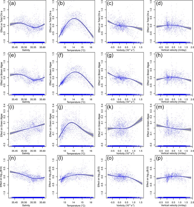
852                                          X. Davila et al.: Coastal mesoscale processes and their effect on phytoplankton

vani et al., 2020). The performance of this system and its          cant bias was present between the measurements of these two
potential for the study of ocean processes and transport pat-       instruments. Once having verified that data can be merged,
terns have already been demonstrated by previous works (e.g.        the optimal statistical interpolation (OSI) was performed by
Rubio et al., 2011, 2018; Solabarrieta et al., 2014; Caballero      the “DAToBJETIVO” software package developed by Gomis
et al., 2020).                                                      and Ruiz (2003) for the objective spatial analysis and the di-
   In order to visualize representative velocity fields, we ap-     agnosis of oceanographic variables.
plied a 10th-order digital Butterworth low-pass filter (Emery          For the interpolation in the sampling area, an 11 × 33 out-
and Thomson, 2001) to both velocity components at each              put grid was used with a 0.031◦ ×0.033◦ resolution (Fig. 1a),
node (filtering out T < 48 h). Therefore, HF processes such         pursuing a compromise between providing a good represen-
as inertial currents or tides were removed, as these are irrel-     tation of the scales that can be resolved by the sampling and
evant for this study and would have eclipsed the geostrophic        minimizing the effect of the observational error. A Gaus-
and wind-induced current mesoscale and submesoscale pat-            sian function for the correlation model between observa-
terns. A Lagrangian particle-tracking model (LPTM) was              tions (assuming 2D isotropy) was set up, with a correlation
applied to HF radar data to simulate trajectories and anal-         length scale of 15 km. The noise-to-signal (NTS) variance
yse surface ocean transport patterns around the dates of the        ratio used for the analysis of temperature, salinity, and dy-
ETOILE survey. Particles released within the HF radar cov-          namic height was 0.01, 0.005, and 0.0027, respectively. This
erage area were advected using a 4th-order Runge–Kutta              ratio was defined as the variance of the observational error
scheme (Benson, 1992). In this case, the particles are ad-          divided by the variance of the interpolated field (the latter re-
vected using the 2D hourly current fields given by the HF           ferring to the deviations between observations and the mean
radar from 26 July to 11 August. To describe (sub)mesoscale         field). This parameter allows the inclusion in the analysis of
patterns, Lagrangian residual currents (LRC) were calculated        an estimation of the observational error and adjustments of
following a methodology similar to that described in Muller         the weight of the observations on the analysis (the larger
et al. (2009) using an integration time of 3 d.                     the NTS parameter, the smaller the influence of the obser-
   Furthermore, satellite data prior to and after the cruise        vation). Following this, i.e. after the interpolation, all fields
were also analysed. Sea surface temperature (SST) and satel-        were spatially smoothed, with an additional low-pass filter
lite chl a data (chl-a sat ) were retrieved from the Visible and    with a cut-off length scale of 10 km to avoid aliasing errors
Infrared Imager/Radiometer Suite (VIIRS) sensor, and wa-            due to unresolved structures. This resulted in a coarse grid
ter turbidity was retrieved from MODIS. In addition to these        that allowed the appropriate representation of the subsequent
datasets, hourly wind information of July and August was            spatial derivatives of the analysed field. In the vertical, 98
collected by the mooring buoy of Bilbao owned by Puertos            equally spaced levels were considered, from 4 to 200 m (ev-
del Estado (available in http://www.puertos.es/en-us, last ac-      ery 2 m). To analyse and correlate the explanatory and the
cess: 11 June 2021). Although its location is not exactly in        response variables, the same interpolation was performed for
our study area (Fig. 1b), it is considered close enough for a       the chl a data.
general description of the wind regime in the bay.
                                                                    2.4   Statistical analysis
2.3   Computation of vorticity and vertical velocities
                                                                    The presence of a well-defined seasonal pycnocline and a
From hydrographic data alone, geostrophic circulation can be        DCM were used as criteria to define three dynamically dif-
diagnosed, inferring various key dynamical variables, such          ferent layers in the water column, which have been analysed
as geostrophic relative vorticity (hereinafter referred to just     separately to constrain the different dynamical environments.
as vorticity) or the vertical velocity from a 3D snapshot of        Therefore, prior to the statistical analysis, the dataset was di-
the density field. To compute vertical velocities, we assume        vided in three subsets: “above the pycnocline” (“APY”, con-
quasi-geostrophic dynamics and a synoptic or steady state,          taining data from 4 to 24 m depth), “below the pycnocline”
where the Rossby number is small (Ro = U/f L  1, where             (“BPY”, containing data from 26 to 74 m depth), and “at the
U is the characteristic velocity, L is length scale, and f is the   DCM” (“DCM”, containing data from 26 to 74 m and where
Coriolis parameter) and submesoscale features remain con-           total chl-a ≥ 1.5 µg ChlaEQL-1).
stant during the sampling (Gomis et al., 2001). To reduce the          We assessed the relative importance of different environ-
computational effort during the analysis of the data, the MVP       mental factors involved in the phytoplankton distribution by
transects were averaged every 5 km, considering it to be a          developing a statistical generalized additive model (GAM)
high enough resolution for resolving submesoscale struc-            (Hastie and Tibshirani, 1990). GAMs offer the possibility of
tures, following the methodology in Gomis et al. (2001). An         identifying non-linear relationship between variables by the
interpolation of the data allows for deriving key dynamical         inclusion of a smoothing function that has no specific shape.
variables, such as the geostrophic relative vorticity and ver-      Since the relationship among variables along the entire wa-
tical velocities. This was accomplished by merging the CTD          ter column might mask each other, three GAMs were imple-
and averaged MVP profiles after verifying that no signifi-          mented for the different dynamical environments in the water

Ocean Sci., 17, 849–870, 2021                                                            https://doi.org/10.5194/os-17-849-2021
X. Davila et al.: Coastal mesoscale processes and their effect on phytoplankton                                                          853

Table 1. Generalized additive model (GAM) results. Intercept, standard error (StE), significance (p value), and explained variance (%) of the
GAMs for the water column sections “Above the pycnocline” (APY), “below the pycnocline” (BPY) and at the deep chlorophyll maximum
(DCM). Dependent variables are the estimated chl a concentrations for the different algae groups, and B : G refers to the brown chl a to green
chl a ratio. The estimated degrees of freedom (edf) and significance (p value) of the environmental variables are also included. Although
salinity and temperature were correlated for the section BPY, both variables were kept since the fit (R 2 and general cross-validation, GCV)
was better in all cases.

                                                            APY                     BPY                     DCM
                                                     Estimate    p value    Estimate      p value   Estimate     p value
                    Total chl a     Intercept          0.380     < 0.001       1.096     < 0.001       1.793     < 0.001
                                    StE               0.0050                  0.0006                  0.0120
                                    %                   60.8                    66.0                    17.3
                                    GCV                0.020                   0.069                   0.051
                                                          edf    p value          edf     p value         edf    p value
                                    Vertical_vel        1.000    < 0.001        2.461    < 0.001       2.618       0.009
                                    Temperature         2.979    < 0.001        2.972    < 0.001       2.851     < 0.001
                                    Vorticity           2.788    < 0.001        2.896    < 0.001       2.744     < 0.001
                                    Salinity            2.990    < 0.001        2.974    < 0.001       2.484     < 0.001
                                                     Estimate    p value    Estimate      p value   Estimate     p value
                    Brown chl a     Intercept          0.206     < 0.001       0.775     < 0.001       1.374     < 0.001
                                    StE               0.0030                  0.0060                  0.0091
                                    %                   57.1                    71.8                    37.7
                                    GCV                0.051                   0.044                   0.030
                                                          edf    p value          edf     p value         edf    p value
                                    Vertical_vel        2.658    < 0.001        2.650    < 0.001       2.844     < 0.001
                                    Temperature         2.988    < 0.001        2.981    < 0.001       2.025       0.093
                                    Vorticity           2.934    < 0.001        2.960    < 0.001       2.816     < 0.001
                                    Salinity            2.983    < 0.001        2.970    < 0.001       2.596       0.004
                                                     Estimate    p value    Estimate      p value   Estimate     p value
                    Green chl a     Intercept          0.148     < 0.001       0.321     < 0.001       0.418     < 0.001
                                    StE               0.0040                  0.0026                  0.0058
                                    %                   43.0                    34.1                    56.9
                                    GCV                0.013                   0.012                   0.012
                                                          edf    p value          edf     p value         edf    p value
                                    Vertical_vel        2.353    < 0.001        1.924    < 0.001       1.000     < 0.001
                                    Temperature         2.983    < 0.001        2.988    < 0.001       2.978     < 0.001
                                    Vorticity           1.000      0.362        2.871    < 0.001       2.263     < 0.001
                                    Salinity            2.986    < 0.001        1.000    < 0.001       2.784     < 0.001
                                                     Estimate    p value    Estimate      p value   Estimate     p value
                    B:G             Intercept          0.109     < 0.001       0.361     < 0.001       0.543     < 0.001
                                    StE               0.0189                  0.0044                  0.0063
                                    %                   55.0                    57.2                    64.5
                                    GCV                0.283                   0.034                   0.015
                                                          edf    p value          edf     p value         edf    p value
                                    Vertical_vel        2.452    < 0.001        2.588    < 0.001       1.866     < 0.001
                                    Temperature         2.996    < 0.001        2.712    < 0.001       2.874     < 0.001
                                    Vorticity           2.572      0.056        2.941    < 0.001       2.652     < 0.001
                                    Salinity            2.983    < 0.001        2.935    < 0.001       2.819     < 0.001

https://doi.org/10.5194/os-17-849-2021                                                                    Ocean Sci., 17, 849–870, 2021
854                                          X. Davila et al.: Coastal mesoscale processes and their effect on phytoplankton

                                                                  three vertical subsets (Table 1). All the variables showed a
                                                                  significant impact on the total and group chl a distribution
                                                                  except the vorticity for the green chl a in the APY subset.
                                                                  If vorticity was removed, the model slightly improved (GCV
                                                                  decreased from 0.0130 to 0.0125; Table 2). However, we de-
                                                                  cided to keep it in the model for the different levels, keeping
                                                                  in mind that its impact in the APY subset was insignificant.
                                                                  In addition, vertical velocities for the APY subset show un-
                                                                  realistic values as an artefact of the surface boundary condi-
                                                                  tion necessary to perform the calculations, where velocities
                                                                  are assumed to be null. Since the derived relationships with
                                                                  chl a are not considered realistic (even if they are included
                                                                  in the analysis and slightly improve the models), they are
                                                                  not considered further. The rest of the variables, even if they
                                                                  explained a small part of the variance, they significantly im-
                                                                  proved the model. The GAMs were carried out by using R
                                                                  (version 3.63, R Core Team, 2020) and the package mgcv
                                                                  (version 1.8.33) (Wood, 2011).

                                                                  3     Results
Figure 2. Wind direction and intensity at Bilbao’s mooring buoy
represented on a progressive vector diagram (PVD).                3.1    Mapping coastal mesoscale hydrography and
                                                                         currents
column, as previously detailed, by using (Eq. 1):
                                                                  The combined use of wind data and satellite imagery together
[chl − a]z = a + g1 [Salz ] + g2 [Tempz ] + g3 [Vorz ]            with the HF radar provides a context of hydrographical and
+ g4 [V.Velz ] + ,                                        (1)    dynamical regime around the dates of the ETOILE cruise.
                                                                  Figure 2 shows the progressive vector diagram (PVD) of the
where (a) is an intercept, z is the location in the water col-    wind conditions. From 21 to 28 July, the predominant wind
umn (APY, BPY, and DCM), g is the nonparametric smooth            has a marked northwesterly component with relatively high
functions describing the effect of environment on chl a con-      intensity. Afterwards, it decreases in intensity, shifts, and
centrations, and  is an error term. Sal, Temp, Vor, and V. Vel   starts blowing from the northeast. On 7 August, the wind
correspond to the environmental variables determined in this      again has a northwest component for few days. Therefore,
study, salinity, temperature, vorticity (cyclonic or anticy-      the wind conditions during the whole cruise remain almost
clonic), and vertical velocities (upwelling or downwelling),      constant in direction and low in intensity. Figure 3 shows the
respectively.                                                     satellite SST, chl-a sat , and turbidity fields; the latter allowed
   In order to account for co-linearity problems, we cal-         us to locate the river plumes of the Adour and the Bidasoa
culated pairwise Spearman correlation coefficients (r) be-        rivers. In addition, the LRC fields derived from the HF radar,
tween variables. The only pair of variables correlated were       which are superimposed onto the previous fields, give a high-
salinity and temperature for the BPY subset (r = −0.77,           resolution image of the surface transport during the days pre-
p value < 0.05) related to the depth dependency of both           vious to the survey in the periods 26–29 July and 30 July to
variables. The model selection was based on the analysis          2 August. The surface circulation patterns and position of
performed by Llope et al. (2009), where a stepwise ap-            the river plumes are observed to evolve from the first to the
proach was implemented by removing covariates and min-            second periods. On 26–29 July (Fig. 3, left column), under
imizing the generalized cross-validation (GCV) criterion of       northwesterly winds the circulation shows complex spatial
the model (Wood, 2000). The GCV criterion is a measure of         patterns, and two cyclonic eddies, with diameters between
the out-of-sample predictive performance of the model and         10–15 km, can be identified (C17W at 43.6◦ N and 2◦ W and
is related to the Akaike information criterion (AIC) (Wood,       C17E at 43.7◦ N and 1.7◦ W). During the period 30 July to
2006). Similarly, by deleting one variable at a time we can       2 August (Fig. 3 – right column), the winds shift to north-
quantify the penalty on the explained variance of the phyto-      easterly, which generates a remarkable transition to westward
plankton distribution (Llope et al., 2009). In total, 12 GAMs     currents. At this moment, the cyclonic eddies are not visible
were carried out from the combination of total chl a, green       to the HF radar. Instead, in their position, we observe a me-
algae chl a (green chl a), brown algae chl a (brown chl a),       andering pattern that affects the distribution of the SST and
and the brown chl a to green chl a ratio (B : G) among the        the position of the river plumes and their associated chl-a sat

Ocean Sci., 17, 849–870, 2021                                                          https://doi.org/10.5194/os-17-849-2021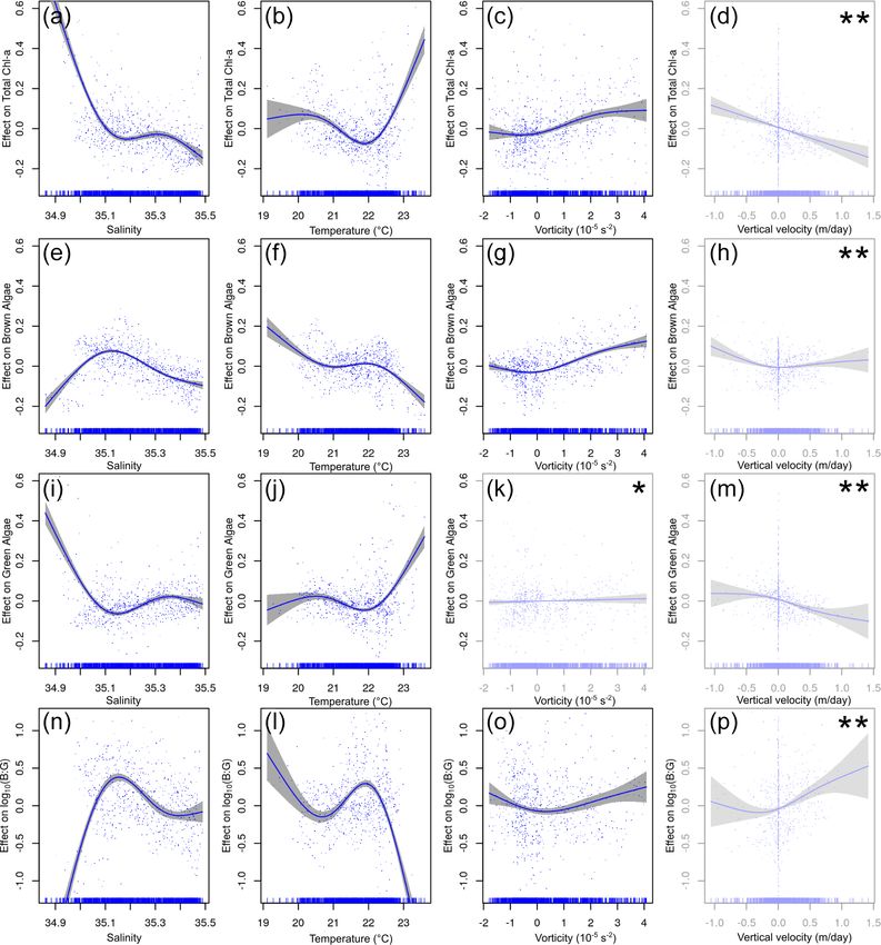
X. Davila et al.: Coastal mesoscale processes and their effect on phytoplankton                                                              855

Figure 3. Satellite observations for SST (a, b), turbidity (c, d), and chl-a sat (e, f) corresponding to 29 July (a, c, e) and 2 August (b, d, f).
Black lines show the Lagrangian residual currents (LRC) calculated for the periods 26–29 July and 30 July to 2 August. The black box shows
the study area, where ETOILE survey took place. The circles in the left column represent the approximate location of the observed cyclonic
eddies (C17W and C17E). Turbidity and chl a are plotted on logarithmic scale.

signature. In addition, on 2 August, a sharp decrease in SST               ity front is observed at the shelf break (i.e. along the 250 m
is observable close to the French inner shelf, which is linked             isobath), with a vertical extension between 50 and 120 m
with the upwelling generated by the northeasterly winds.                   (Fig. 5). Fresher waters, with salinities of ∼ 35.5 occupy the
   During the ETOILE cruise (2 to 4 August), the first metres              totality of the water column over the shelf, while oceanic wa-
of the water column are characterized by a high spatial vari-              ters at the slope are characterized by salinities over ∼ 35.6.
ability (Fig. 4). Although the river plume is no longer visible            The salinity range in the shelf break front is much smaller
in the salinity fields at 14 m, a layer of relatively fresh water          than in the surface front.
is located in the inner continental shelf (1.6–1.7◦ W). This                  The cyclones depicted in Fig. 3 are also observed at deeper
low salinity front extends over 20 km horizontally and 18 m                layers in the vorticity and geostrophic velocities fields, while
vertically (Fig. 5a) if we consider the isopycnal 35.1 as in               they do not have a clear surface signature during the days of
Puillat et al. (2006). At 60 m depth (Fig. 4), a second salin-             the cruise. The disappearance of the C17W and C17E in the

https://doi.org/10.5194/os-17-849-2021                                                                       Ocean Sci., 17, 849–870, 2021

856                                             X. Davila et al.: Coastal mesoscale processes and their effect on phytoplankton

Figure 4. Synoptic plots for the hydrographic and hydrodynamical conditions for the period (2 to 4 August 2017). From top to bottom the
following variables are shown: salinity, temperature, vorticity, and vertical velocity fields, at 14, 30, and 60 m (left to right). Black arrows
correspond to the geostrophic velocities, and black contours represent the 200 and 250 m isobaths. The dashed white line corresponds to the
cross section at 43.77◦ N shown in Figs. 5 and 7. Negative vorticity values represents anticyclonic circulation, while positive values represent
cyclonic circulation. Negative (positive) vertical velocity values represent downwelling (upwelling). The red (blue) circles drawn in the left
column represent the approximate location of A17 (C17W and C17E). The scale range for each of the variables is different for each depth.

LRC fields during the cruise period coincides with a change               cal velocities), whose maxima have a relatively constant po-
in the wind pattern, which results in a surface wind-driven               sition throughout the water column.
flow that masks the geostrophic circulation at the surface.                  From the cross section at 43.77◦ N, we can observe the ver-
A few days later, once the wind changes back to a north-                  tical extension of both the low salinity surface front and the
west component, C17W is observable again in the HF radar                  shelf break salinity front (Fig. 5a). The surface salinity front
(see Fig. A1), suggesting a persistent nature. It is noteworthy           has a vertical extension of ∼ 20 m, while the location of the
that the vorticity fields also show an anticyclone (A17) at the           shelf break front is at ∼ 50–110 m. The uplift and depres-
northwest part of the domain (centred at 43.80◦ N 2.25◦ W),               sion of the isopycnal lines (black contours) is coherent with
although this is not observed in the HF radar fields. In addi-            the presence of submesoscale structures of different polar-
tion to A17, a region of anticyclonic vorticity is well defined           ity, which mostly follow the temperature distribution. These
in the frontal area between the cyclones. At 60 m the cyclonic            two variables contribute to the water density and the posi-
eddies present a negative temperature anomaly and relative                tion of the seasonal pycnocline at ∼ 25 m, primarily condi-
higher salinity values. A17 is associated with a positive tem-            tioned by the warming of surface waters in summer. From
perature anomaly and higher salinity. Associated with the                 the vorticity field and the geostrophic meridional velocities
frontal areas in the two dipoles (A17–C17W and C17W–                      (Fig. 5d), it is noticed that the position of the anticyclonic
C17E) we observe two main upwelling areas (positive verti-                frontal area between C17W and C17E coincides with the
                                                                          shelf break (1.9◦ W), and its strength decreases with depth

Ocean Sci., 17, 849–870, 2021                                                                    https://doi.org/10.5194/os-17-849-2021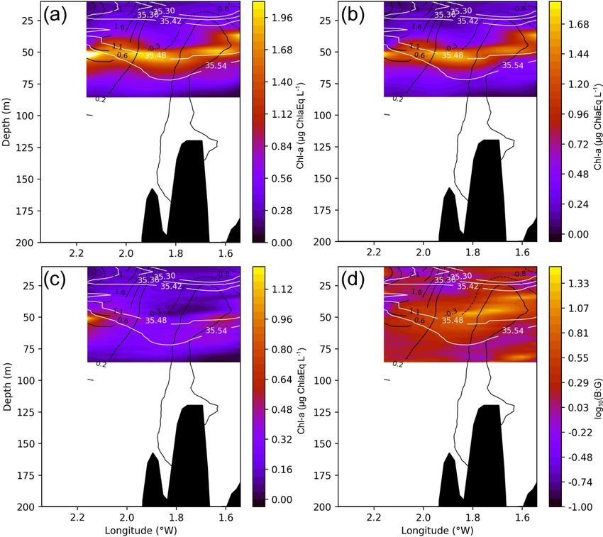
X. Davila et al.: Coastal mesoscale processes and their effect on phytoplankton                                                           857

Figure 5. Cross section at 43.77◦ N (location marked by dashed lines in Figs. 1 and 4), representing salinity (a) and temperature (b) with
isopycnals (black and white contours, respectively) and vorticity (c) and vertical velocities (d) with meridional geostrophic velocities (solid
(dashed) black contours for positive (negative) velocities) for the period (2 to 4 August 2017). Negative vorticity values represents an-
ticyclonic circulation, while positive values represent cyclonic circulation. Positive (negative) values for geostrophic velocity represent a
northward (southward) current. Negative (positive) vertical velocity values represent downwelling (upwelling). The red (blue) horizontal
lines represent the horizontal extension of A17 (C17E) that the section crosses.

from a maximum at 25 m. The onshore area is dominated by                  served, one over the inner shelf at ∼ 30–50 m, and the second
a southward flow while the offshore area is dominated by a                over the shelf edge at ∼ 50–65 m, which is below the pycno-
northward flow. As in Fig. 4, the highest vertical velocities             cline. The shallow DCM is split into two cores, although its
are located in the eddies’ periphery, where the largest vortic-           morphology is hard to assess due to the limited spatial cov-
ity gradients are located.                                                erage of the sampling. The deep DCM is located at the anti-
                                                                          cyclonic frontal area between C17W and C17E and is com-
3.2   Chlorophyll a and spectral group distribution                       posed of mainly brown algae, the dominant spectral group.
                                                                          The maximum is centred in the anticyclonic frontal area be-
                                                                          tween C17W and C17E. Green algae, however, follow a dif-
Surface chl a (from the continuous recording surface Fluo-
                                                                          ferent pattern and are distributed slightly deeper, following
roprobe) shows a distribution that is spatially dependent on
                                                                          the salinity contours over 35.55. The ratio between brown
salinity at 3.5 m depth, related to the position of the river
                                                                          chl a and green chl a (B : G), logarithmically transformed,
plume (Fig. 6). The chl a maximum is observed around
                                                                          provides an even clearer image of how the different spectral
the salinity minimum, decreasing to the northwest (and with
                                                                          groups are distributed. There is a sharp transition between
depth) in accordance with the increase of salinity. Vertically,
                                                                          the brown algae (around the anticyclonic frontal area) and
the 43.77◦ N cross section shows a complex distribution of
                                                                          the green algae (below the 35.55 isohaline). The 43.70◦ N
total chl a and spectral groups (Fig. 7). Two DCMs are ob-

https://doi.org/10.5194/os-17-849-2021                                                                     Ocean Sci., 17, 849–870, 2021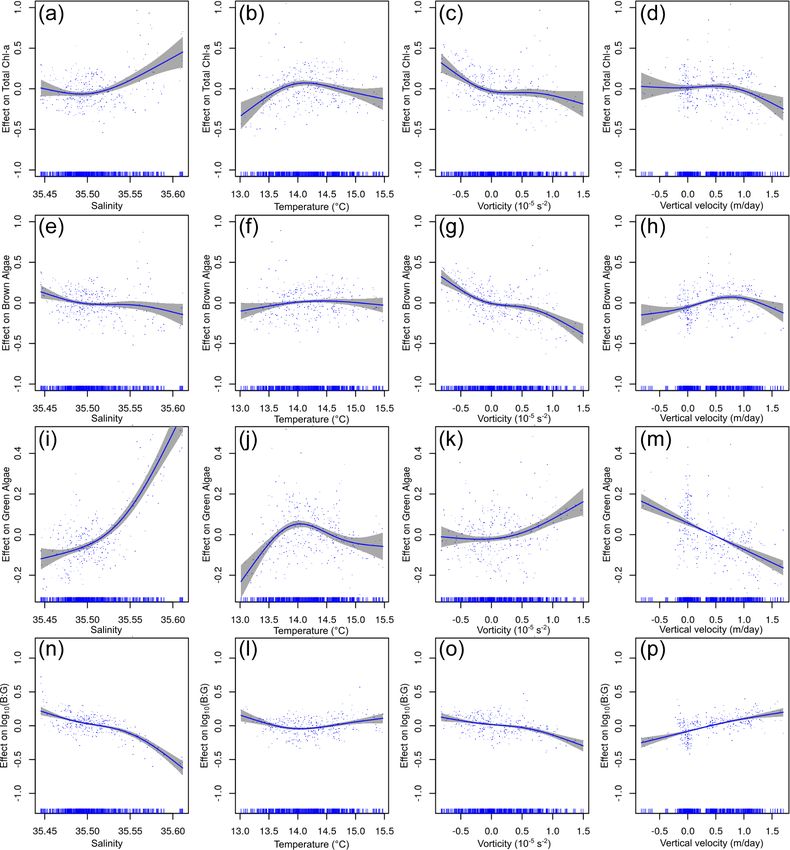
858                                             X. Davila et al.: Coastal mesoscale processes and their effect on phytoplankton

                                                                        the APY subset (except for the green algae) and suggest a
                                                                        different response of the chl a to the environmental vari-
                                                                        ables (Table 1, Fig. 9). We observe a negative correlation
                                                                        between chl a and salinity until values of ∼ 35.5 (Fig. 9a)
                                                                        and a dome-shaped behaviour with temperature (34 % of ex-
                                                                        plained variance), with a maximum at ∼ 14 ◦ C (Fig. 9b, Ta-
                                                                        ble 2). Although the explained variance by vorticity is small,
                                                                        there is a clear positive trend in chl a with negative or anti-
                                                                        cyclonic vorticity (Fig. 9c). Again, brown chl a mimics the
                                                                        responses of the total chl a (temperature explains most of the
                                                                        variance, 27.30 %). Green chl a shows a positive linear rela-
Figure 6. Surface chl a at 3.5 m from the surface Fluoroprobe for
the period (2 to 4 August 2017). White contours represent the salin-    tionship with salinity (Fig. 9i) and a dome-shaped distribu-
ity field, while black contours represent the 200 and 250 m isobaths.   tion with temperature (Fig. 9j, 19 % of explained variance),
The red (blue) circles in the left column represent the approximate     with a maximum at slightly colder waters. The B : G ratio
location of A17 (C17W and C17E).                                        (Fig. 9n) shows a negative correlation with salinity (11.80 %
                                                                        of explained variance), while temperature has a lower impact
                                                                        (4.50 % of explained variance).
cross section (see Fig. A2), which does not cross the core of              While the GAMs at the DCM subset perform substantially
the anticyclonic front, reveals that this pattern is not ubiq-          worse for the total chl a (only 17.3 % of explained vari-
uitous. Here, there is neither a clear dichotomy among the              ance), they show much better performances for brown and
groups nor a deeper maximum of green algae.                             green chl a distributions, with 37.7 % and 56.9 % of the ex-
                                                                        plained variance, respectively. The model for the B : G ratio
3.3   Exploring bio-physical impacts                                    explains an even higher percentage of the variance (64.5 %).
                                                                        Total chl a distribution is correlated with salinity and vortic-
The results of the GAMs in the APY subset (Fig. 8, Table 1)             ity (Fig. 10a and c) and shows a dome-shaped relationship
suggest that, overall, all of the models perform well, explain-         with temperature (Fig. 10b) similar to that of APY and BPY
ing in all cases more than 40 % of the variance. Salinity and           subsets. However, the relative importance of the variables is
temperature contribute to most of the variance of the model             different, vorticity explains the 9.97 % of the variance and is
and explain 13.10 % and 9.8 % of it, respectively (Table 2).            depicted as the main modulating environmental factor; how-
As expected, in agreement with Fig. 6, lower salinity values            ever, this is very close to the 8.98 % explained by salinity.
are associated with higher total chl a concentration, show-             These differences are reinforced for the brown chl a model,
ing a negative relationship (Fig. 8a). Regarding the effect             where salinity and temperature explain a very low percent-
of temperature, it follows a convex-shaped function, with a             age of the variance (with almost flat distributions, Fig. 10e–
minimum at ∼ 22 ◦ C (Fig. 8b), while the contribution of vor-           f), and vorticity and vertical velocity are responsible of the
ticity (Fig. 8c) is very small. The response of brown chl a             19.30 % and 4.40 % of the variance, respectively (Table 2).
differs from total chl a, although salinity still explains most         For the green chl a, the main modulating factors are salinity
of the variance of the model (23.3 %). Brown chl a shows                and vertical velocity (Fig. 10i and m, 25.40 % and 10.5 % of
a dome-shaped response to salinity (Fig. 8e) with a maxi-               explained variance, respectively), while the effect of vortic-
mum at ∼ 35.1 (i.e. waters fresher or saltier than 35.1 have            ity is very low (Fig. 10k, 4.10 %). In the case of DCM green
a negative impact) and a positive response to positive (cy-             chl a distribution, positive values of vertical velocity (up-
clonic) vorticity. Green chl a almost mimics the distribution           welling) impact the chl a concentration negatively. Finally,
of total chl a (Fig. 8i–m), except for the non-significant rela-        for the B : G ratio, salinity stands out as the main modulating
tion with vorticity (p value > 0.05). For green algae, tem-             factor, explaining 20 % of the variance. However, the effect
perature and salinity explain 10.40 % and 12.70 % of the                of vertical velocities and vorticity is also considerable, with
variance, respectively. Note that in this case the removal of           14 % and 9.30 % of explained variance, respectively.
salinity has no penalty in the explained variance, likely ow-
ing to the temperature capturing most of the variability. The
B : G ratio shows dome-shaped relationships for salinity and            4   Discussion
temperature, where the maxima are at ∼ 35.2 and ∼ 22 ◦ C
(Fig. 8n and l). In fresher and/or warmer waters, higher con-           During and around the dates of the ETOILE oceanographic
centrations of green algae are observed. The contributions of           cruise, two cyclones (C17W and C17E) were observed in
both salinity and temperature to the variance are similar, i.e.         the study area by means of different multiplatform sensors.
15.6 % and 15.8 %, respectively.                                        While the signature of the cyclones in the HF radar fields was
   In the BPY subset, the GAMs explain a larger percent-                not continuous (and dependent on the prevailing wind con-
age of the variance and generally perform better than for               ditions), their subsurface structure could be diagnosed from

Ocean Sci., 17, 849–870, 2021                                                               https://doi.org/10.5194/os-17-849-2021
Table 2. Variance contribution of the environmental variables to the estimated chl a concentrations for the different algae groups; brown : green (B : G) ratio; and the “above the
pycnocline” (APY), “below the pycnocline” (BPY), and at the deep chlorophyll maximum (DCM) subsets. The left columns in each of the sections show these values for the models
after stepwise deletion of the variables listed to the left (first the vertical velocities and then the temperature). The coefficient of determination (R 2 ), general cross-validation score
(GCV), and the percentage of variance (%) correspond to the different models. The last two models included only the variable listed (vorticity or salinity). For the right columns in each
section, one variable (those listed on the left) was removed at a time while keeping the rest. While R 2 and GCV still refer to the whole model, percentage of variance is individual and
corresponds only to the removed variable. Bold numbers point out the main modulating variable, i.e. the one that individually explains most of the variance in the model.
APY BPY DCM
https://doi.org/10.5194/os-17-849-2021
Stepwise deletion Delete one covariance Stepwise deletion Delete one covariance Stepwise deletion Delete one covariance
R2 GCV % R2 GCV % R2 GCV % R2 GCV % R2 GCV % R2 GCV %
Total chl a All (total) 0.60 0.020 0.66 0.069 0.15 0.052
Vertical_vel 0.59 0.021 1.40 0.59 0.021 1.40 0.65 0.070 0.60 0.65 0.070 0.60 0.12 0.055 3.40 0.12 0.055 3.40
Temperature 0.46 0.027 58.91 0.51 0.025 9.80 0.32 0.138 34.20 0.32 0.138 34.00 0.08 0.057 7.88 0.09 0.057 6.30
Vorticity 0.02 0.077 11.50 0.58 0.022 2.50 0.06 0.184 59.62 0.64 0.073 2.10 0.05 0.058 11.07 0.06 0.059 9.97
Salinity 0.46 0.027 14.40 0.47 0.042 13.10 0.30 0.140 35.50 0.64 0.073 2.20 0.02 0.060 15.45 0.07 0.058 8.98
Brown chl a All (total) 0.56 0.005 0.72 0.044 0.36 0.031
Vertical_vel 0.55 0.005 1.20 0.55 0.005 1.20 0.71 0.046 0.70 0.71 0.046 0.70 0.32 0.033 4.40 0.32 0.032 4.40
Temperature 0.46 0.006 10.30 0.49 0.006 7.50 0.44 0.088 27.70 0.44 0.087 27.30 0.30 0.033 6.60 0.35 0.031 0.70
Vorticity 0.29 0.008 28.00 0.44 0.007 12.40 0.09 0.143 63.11 0.68 0.051 4.00 0.26 0.035 11.10 0.17 0.039 19.30
Salinity 0.14 0.010 43.30 0.33 0.008 23.30 0.42 0.091 29.70 0.63 0.058 8.80 0.08 0.043 28.69 0.34 0.032 1.60
Green chl a All (total) 0.42 0.013 0.01 0.56 0.012
X. Davila et al.: Coastal mesoscale processes and their effect on phytoplankton
Vertical_vel 0.40 0.013 2.00 0.40 0.013 2.00 0.33 0.012 1.3 0.33 0.012 1.3 0.46 0.015 10.50 0.46 0.015 10.5
Temperature 0.30 0.015 12.70 0.32 0.015 10.40 0.13 0.015 20.5 0.14 0.015 19.90 0.43 0.016 13.00 0.50 0.014 6.00
Vorticity 0.01 0.044 41.64 0.42 0.013 0.00 0.04 0.017 30.15 0.64 0.073 2.10 0.21 0.022 36.20 0.52 0.014 4.10
Salinity 0.30 0.015 12.70 0.43 0.026 0.00 0.01 0.016 24.56 0.31 0.012 2.80 0.37 0.017 19.20 0.30 0.020 25.40
B:G All (total) 0.54 0.283 0.57 0.034 0.64 0.015
Vertical_vel 0.53 0.289 1.30 0.53 0.289 1.30 0.56 0.035 1.00 0.56 0.035 1.00 0.50 0.020 14.00 0.50 0.020 14.00
Temperature 0.37 0.385 17.30 0.39 0.379 15.80 0.51 0.038 5.80 0.53 0.038 4.50 0.50 0.020 14.20 0.60 0.016 3.40
Vorticity 0.02 0.657 52.46 0.54 0.287 1.00 0.08 0.721 48.58 0.53 0.037 4.20 0.30 0.028 34.10 0.54 0.018 9.30
Salinity 0.63 0.392 18.70 0.39 0.414 15.60 0.48 0.409 9.10 0.45 0.043 11.80 0.32 0.027 31.70 0.43 0.023 20.00
Ocean Sci., 17, 849–870, 2021
859860 X. Davila et al.: Coastal mesoscale processes and their effect on phytoplankton
Figure 7. Cross section at 43.77◦ N (location marked by dashed lines in Figs. 1 and 4; same section as in Fig. 5) of total chl a (a), brown
chl a (b), green chl a (c), and the brown chl a to green chl a ratio (B : G), which has been logarithmically transformed (d) for the chosen
period (2 to 4 August 2017). White lines represent salinity contours, and solid black lines represent positive vorticity values or cyclonic
circulation, while dashed lines represent negative vorticity values of anticyclonic circulation. The red and blue horizontal lines represent the
horizontal extension of A17 and C17E, respectively, that the section crosses.
the hydrographic measurements obtained during the cruise. brown and green chl a, vorticity captures most of the vari-
The geostrophic circulation indicated the presence of a dipole ance in the DCM for brown algae.
structure formed by C17W and C17E, a frontal region of an-
ticyclonic circulation in between, and an additional anticy- 4.1 Physical environment
clone (A17). Further, two salinity fronts were observed, one
near the surface (< 14 m) and one at the subsurface (> 50 m). The hydrographic and hydrodynamic regimes observed at
From the chl a profiles, the DCM could be located below the the SE-BoB during the ETOILE cruise, despite being spatio-
pycnocline at ∼ 60 m, while the chl a distribution of the two temporally highly complex, were not exceptional and similar
dominant spectral groups of algae, brown and green algae, conditions have been already recorded. The surface salinity
was depicted. The relative importance of the environmental front we encountered onshore was observed on early May
factors modulating the chl a distribution was assessed by the 2009 by Reverdin et al. (2013). They described a fresher (34–
use of GAMs. The GAMs not only showed that these en- 35) and deeper (∼ 30 m) freshwater layer originated due to
vironmental factors affect the brown and green algae differ- winter and spring river runoff and which signal weakens to-
ently but also that their relative importance changes through- wards August by increasing salinity to ∼ 35, as a result of
out the water column. While salinity and temperature explain vertical mixing and offshore advection by Ekman transport.
most of the variance above and below the pycnocline of both This shelf break front is a recurrent feature in the study area,
and is originated by the differences between the waters over
Ocean Sci., 17, 849–870, 2021 https://doi.org/10.5194/os-17-849-2021X. Davila et al.: Coastal mesoscale processes and their effect on phytoplankton 861 Figure 8. The relationship between environmental variables and chl a from the above the pycnocline (APY) subset GAMs. The y axis indicates the additive effect that the term on the x axis has on the chl a. The variables are given in the following order (from top to bottom): total chl a, brown chl a, green chl a, and the brown chl a to green chl a ratio (B : G). The shaded area represents the confidence interval of 95 %. The effect of vorticity for green algae chl a is the only non-significant response (marked by ∗ ). The effect of vertical velocity is shown here but is not analysed further since this variable is strongly influenced (in the APY subset) by the proximity to the surface layer boundary condition assumed for its calculation (marked by ∗∗ ). https://doi.org/10.5194/os-17-849-2021 Ocean Sci., 17, 849–870, 2021
862                                            X. Davila et al.: Coastal mesoscale processes and their effect on phytoplankton

Figure 9. Relationship between environmental variables and chl a from the below the pycnocline (BPY) subset GAMs. The y axis indicates
the additive effect that the term on the x axis has on the chl a. The following variables are shown (from top to bottom): total chl a, brown
chl a, green chl a, and the brown : green (B : G) ratio. The shaded area represents the confidence interval of 95 %.

Ocean Sci., 17, 849–870, 2021                                                                 https://doi.org/10.5194/os-17-849-2021
X. Davila et al.: Coastal mesoscale processes and their effect on phytoplankton                                                            863

Figure 10. Relationship between environmental variables and chl a from the deep chlorophyll maximum (DCM) subset GAMs. The y axis
indicates the additive effect that the term on the x axis has on the chl a. The following variables are shown (from top to bottom): total chl a,
brown chl a, green chl a, and the brown : green (B : G) ratio. The shaded area represents the confidence interval of 95 %.

https://doi.org/10.5194/os-17-849-2021                                                                      Ocean Sci., 17, 849–870, 2021
864                                         X. Davila et al.: Coastal mesoscale processes and their effect on phytoplankton

the French shelf and the Landes Plateau and those located         currents to progressively become the main driver for parti-
over the Spanish shelf and slope (Valencia et al., 2004).         cle advection. These two layers are also different regarding
   Furthermore, the dipole-type structures have also been ob-     the nutrient supply. Typically, waters above the mixed layer
served before in the BoB, yet in a larger scale (Pingree and      are depleted in nutrients, whereas below this point the phy-
Garcia-Soto, 2014; Solabarrieta et al., 2014; Caballero et al.,   toplankton would benefit from the nutrient supply via ocean
2016; Rubio et al., 2018). Both the location of the vertical      deep waters in combination with maximum light penetration
velocities at the periphery of the structures and the magni-      in summer (Cullen, 2015). This can also lead to different
tude (1–10 m d−1 ) are consistent with already reported re-       phytoplankton communities with different nutrient require-
sults (Mahadevan et al., 2008; Lévy et al., 2012; Caballero       ments.
et al., 2016). While the cyclones were detected by the HF            At APY, most of the variance of total and brown chl a is
radar before the cruise, these were vanished during the sur-      explained by salinity, while the environmental variable that
vey due to the change in the wind-induced current regime.         explains most of the green chl a variance is temperature.
Their intermittent signature in the HF radar surface fields       These results suggest that the green algae is likely associ-
is explained by the interaction of the geostrophic and wind-      ated with the presence of nutrients on river plumes (fresher
induced flow. A similar situation was described using an an-      and warmer waters) from Adour and Bidasoa. However, the
alytical model in the Florida current by Liu et al. (2015),       brown algae seemed to be unaffected by the river plume, at
where a surface meandering flow was observed as a result          least directly, since they display high chl a concentration at
of the overlap between a coastal jet and an eddy dipole field.    deeper, colder, and slightly saltier waters. The causative link
This is coherent with our observations, i.e. under predom-        between the environmental variables and the brown chl a
inant NE winds the wind-driven circulation over the eddy          distribution is harder to draw. However, salinity is the main
field results in a meandering structure. Indeed, as the wind      modulating factor and might suggest an indirect link with
weakens the cyclones signature is again observed in the HF        nutrient provisioning by river runoff. At BPY, temperature is
radar fields, highlighting the importance of using a wide         the variable that explains most of the variance. However, this
range of multiplatform spatio-temporal data for a better char-    could be the result of the positioning of the DCM at a spe-
acterization of the coastal hydrodynamics.                        cific depth and the large vertical gradient of temperature in
                                                                  the water column, where there would be a good compromise
4.2   Environmental drivers                                       between light and nutrient availability (not measured during
                                                                  this study) for phytoplankton growth (Cullen, 2015). In fact,
In the BoB, coastal chl a is highly dependent on the sea-         for the B : G ratio, this effect cancels out, and salinity is the
sonality of riverine nutrient inputs (Guillaud et al., 2008;      most important environmental factor. Overall, when integrat-
Borja et al., 2016; Muñiz et al., 2019). From satellite im-       ing the entire water column, even though the responses differ
agery and continuously recorded surface salinity and chl-a sat    in the different subsets, salinity is the most important envi-
data (Figs. 3 and 6), it is evident that the Adour and Bidasoa    ronmental factor regarding the total chl a distribution and the
plumes are associated with the highest chl a concentrations       relative occurrence of brown and green algae. We attribute
at the sea surface. Simultaneously, the location of the Adour     this effect to salinity and its relation to nutrient content at
and Bidasoa plumes depends on the wind conditions, which          the surface (with fresher water) and at depth (saltier waters)
control the non-geostrophic surface circulation, as shown by      (Muñiz et al., 2019).
the HF radar LRC. Our results agree with the observed gen-           At the DCM, vorticity is the factor that explains most of
eral pattern in which westerly winds push the river plume         the variance in total chl a and brown chl a concentrations.
towards the coast, while easterly winds promote an offshore       The more negative (positive) the vorticity, the more anticy-
expansion (Petus et al., 2014). Thereby, the uppermost chl a      clonic (cyclonic) the circulation and the more positive (neg-
pattern is eventually dependent on the winds that modulate        ative) the effect on brown chl a concentrations. In anticy-
the position of the river plume. At the subsurface, the occur-    clones, due to Ekman transport, a small part of the flow tar-
rence of the DCM agrees with previously described phyto-          gets the core, leading to an accumulation of phytoplankton
plankton distributions. Muñiz et al. (2019) described a DCM       at their centre (Mahadevan et al., 2008). In contrast, Ekman
below 30 m in summer at the same sector on the BoB. Ca-           transport results in outward transport in cyclones. Therefore,
ballero et al. (2016) also reported a summer DCM at around        C17W and C17E would have advected the brown algae and
40 m (below the thermocline) at the periphery of two cy-          expelled them from the core. These were then subsequently
clones.                                                           trapped in the anticyclonic circulation located between the
   Between the uppermost layer and the pycnocline, non-           cyclones. A similar pattern is described by Caballero et al.
geostrophic processes related to wind-driven currents (e.g.       (2016), where the highest chl a concentrations were located
offshore advection of coastal waters during upwelling-            at the periphery of the cyclones. The effect of this advec-
favourable winds) have an important role in the chl a distri-     tion by submesoscale processes is such that the distribution
bution changes, showing decreasing intensity with depth. In       of brown algae at the DCM cannot be statistically explained
contrast, below the pycnocline, we could expect geostrophic       without the addition of vorticity to the GAM.

Ocean Sci., 17, 849–870, 2021                                                          https://doi.org/10.5194/os-17-849-2021
X. Davila et al.: Coastal mesoscale processes and their effect on phytoplankton 865
However, the distribution of green chl a is not affected concern a relatively small fraction of the total area, may be
by vorticity, and the environmental factor that exerts most disproportionately important to biological dynamics.
of the difference between the two spectral groups is salin-
ity. From our observation we cannot explain the occurrence
of a single spectral group in the core of the anticyclonic cir- 5 Conclusions
culation. Latasa et al. (2017) demonstrated that, during the
We analysed multi-platform in situ and remote sensing data
summer stratification in the Iberian Shelf and Iberian Margin,
to characterize coastal submesoscale processes and their in-
the DCMs are composed of different types of phytoplankton,
fluence on the distribution of the two major phytoplankton
each adapted to the different existing micro-environments.
pigmentary groups in the SE-BoB. Satellite imagery and HF
However, the phytoplankton landscapes organized in sub-
radar data provided information about the uppermost layer,
mesoscale patches are often dominated by a single species
which was highly conditioned by the run-off of Adour and
(D’Ovidio et al., 2010). This structuring of the phytoplankton
Bidasoa rivers. The location of the plume was influenced by
community is a direct effect of the horizontal stirring, which
the surface currents, which are ultimately conditioned by the
can create intense patchiness in species distribution (Lévy
speed and direction of the wind.
et al., 2012). We believe that the observed submesoscale pro-
Multi-spectral chl a fluorescence measurements allowed
cesses during the ETOILE cruise would have perturbed an
us to identify the contrasting effects of a set of environmen-
already existing horizontal layer of DCM, not enhancing pri-
tal variables on the distribution and concentration of different
mary production (not measured during our study) by them-
phytoplankton spectral groups. From top to bottom, salinity
selves but rather isolating, advecting, and gathering the phy-
explained most of the distribution of the chl a for both brown
toplankton in the region of anticyclonic circulation.
and green algae. While salinity would still be the most im-
portant environmental driver for green algae at the DCM,
4.3 Limitations of this study
vorticity explained most of the variance of the distribution of
total chl a and brown chl a at this layer. Anticyclonic circula-
It is worth stating the main limitations encountered during
tion gathered the brown algae in the centre via Ekman trans-
this study, especially focusing on the ETOILE cruise. The
port. The effect was such that the distribution of brown algae
sampling area was insufficient to completely cover some of
within the DCM could not be statistically explained with-
the observed structures. Similarly, having just a synoptic im-
out the vorticity as an environmental variable. This research
age of the processes and lacking temporal information (de-
brings the relevance of the dynamic variables in the study
spite operational and remote sensing data) makes it chal-
of phytoplankton into consideration, as well as the measure-
lenging to derive a cause–consequence relation, especially
ments of multi-spectral chl a fluorescence at high spatial res-
regarding the evolution of the system. Although we used
olution. Further research providing a more detailed composi-
chl a as a proxy for phytoplankton biomass concentration,
tion of the phytoplankton community in terms of pigments,
we note that photo-acclimation of pigment content (Cullen,
size classes, and taxonomy, together with an exhaustive anal-
2015), together with variable fluorescence to chlorophyll ra-
ysis of the hydrodynamics, will help to better identify the
tios (Estrada et al., 1996; Kruskopf and Flynn, 2006; Houliez
ecological and functional traits of phytoplankton groups and
et al., 2012), could lead to elevated chl a concentration rela-
determine their submesoscale distribution in coastal systems.
tive to phytoplankton biomass at depth.
In addition, no further phytoplankton classification was
carried out, which might have helped in defining specific
environmental niches (D’Ovidio et al., 2010; Latasa et al.,
2017) and correlating spectral groups to pigmentary groups
and/or taxa. The latter is an essential issue to be consid-
ered, since the Fluoroprobe factory fingerprints are deter-
mined on mono-specific cultures or target micro-algae that
are not necessarily representative to our shelf and ocean sys-
tem (Houliez et al., 2012). No nutrient or light measurements
were taken either; therefore, we cannot explicitly describe
any inter-species competition, which would have helped us in
understanding the ecological consequences of these subme-
soscale processes. A distinct spectral community structure
was still detected, when compared to the surrounding wa-
ters, which could potentially be extended through the trophic
web and even affect predator foraging behaviour (Cotté et al.,
2015; Tew Kai et al., 2009). Thus, our results suggest that the
combined effects of submesoscale features, even though they
https://doi.org/10.5194/os-17-849-2021 Ocean Sci., 17, 849–870, 2021You can also read