Incorporating canopy structure from simulated GEDI lidar into bird species distribution models - IOPscience
←
→
Page content transcription
If your browser does not render page correctly, please read the page content below
Environmental Research Letters

PAPER • OPEN ACCESS

Incorporating canopy structure from simulated GEDI lidar into bird
species distribution models
To cite this article: Patrick Burns et al 2020 Environ. Res. Lett. 15 095002

View the article online for updates and enhancements.

                                This content was downloaded from IP address 46.4.80.155 on 22/10/2020 at 01:36
Environ. Res. Lett. 15 (2020) 095002 https://doi.org/10.1088/1748-9326/ab80ee
Environmental Research Letters
PAPER
Incorporating canopy structure from simulated GEDI lidar into bird
OPEN ACCESS
species distribution models
RECEIVED
28 August 2019 Patrick Burns1,7, Matthew Clark2, Leonardo Salas3, Steven Hancock4, David Leland5,
REVISED Patrick Jantz1, Ralph Dubayah6 and Scott J Goetz1
7 February 2020
1
ACCEPTED FOR PUBLICATION
School of Informatics, Computing and Cyber Systems, Northern Arizona University, Flagstaff, AZ, United States of America
2
18 March 2020 Geography, Environment and Planning, Sonoma State University, Rohnert Park, CA, United States of America
3
Point Blue Conservation Science, Petaluma, CA, United States of America
PUBLISHED 4
20 August 2020 School of Geosciences, The University of Edinburgh, Edinburgh, United Kingdom
5
Madrone Audubon Society, Santa Rosa, CA, United States of America
6
Department of Geographical Sciences, University of Maryland, College Park, MD, United States of America
Original content from 7
Author to whom any correspondence should be addressed.
this work may be used
under the terms of the E-mail: Patrick.Burns@nau.edu
Creative Commons
Attribution 4.0 licence. Keywords: bird species distribution models, GEDI, lidar, canopy structure, machine learning
Any further distribution
of this work must
Supplementary material for this article is available online
maintain attribution to
the author(s) and the title
of the work, journal
citation and DOI. Abstract
The Global Ecosystem Dynamics Investigation (GEDI) lidar began data acquisition from the
International Space Station in March 2019 and is expected to make over 10 billion measurements
of canopy structure and topography over two years. Previously, airborne lidar data with limited
spatial coverage have been used to examine relationships between forest canopy structure and
faunal diversity, most commonly bird species. GEDI’s latitudinal coverage will permit these types
of analyses at larger spatial extents, over the majority of the Earth’s forests, and most importantly in
areas where canopy structure is complex and/or poorly understood. In this regional study, we
examined the impact that GEDI-derived Canopy Structure variables have on the performance of
bird species distribution models (SDMs) in Sonoma County, California. We simulated GEDI
waveforms for a two-year period and then interpolated derived Canopy Structure variables to three
grid sizes of analysis. In addition to these variables, we also included Phenology, Climate, and other
Auxiliary variables to predict the probability of occurrence of 25 common bird species. We used a
weighted average ensemble of seven individual machine learning models to make predictions for
each species and calculated variable importance. We found that Canopy Structure variables were,
on average at our finest resolution of 250 m, the second most important group (32.5%) of
predictor variables after Climate variables (35.3%). Canopy Structure variables were most
important for predicting probability of occurrence of birds associated with Conifer forest habitat.
Regarding spatial analysis scale, we found that finer-scale models more frequently performed better
than coarser-scale models, and the importance of Canopy Structure variables was greater at finer
spatial resolutions. Overall, GEDI Canopy Structure variables improved SDM performance for at
least one spatial resolution for 19 of 25 species and thus show promise for improving models of
bird species occurrence and mapping potential habitat.
1. Introduction the number of species threatened from extinction
now reaches an unprecedented 1 million, rates of
Due to the widespread impacts of land cover extinction are accelerating, and current actions are
change, pollution, wildlife exploitation, and climate insufficient to reverse these trends (IPBES 2019).
change on species and ecosystems across the world, Monitoring biodiversity across large areas through
biodiversity assessment and monitoring is imperative. rapid, scalable, and accurate remote sensing meth-
The United Nations’ latest global assessment report ods will greatly improve our understanding of species
on biodiversity and ecosystem services estimates that distributions, loss and resilience, drivers of changes,
© 2020 The Author(s). Published by IOP Publishing Ltd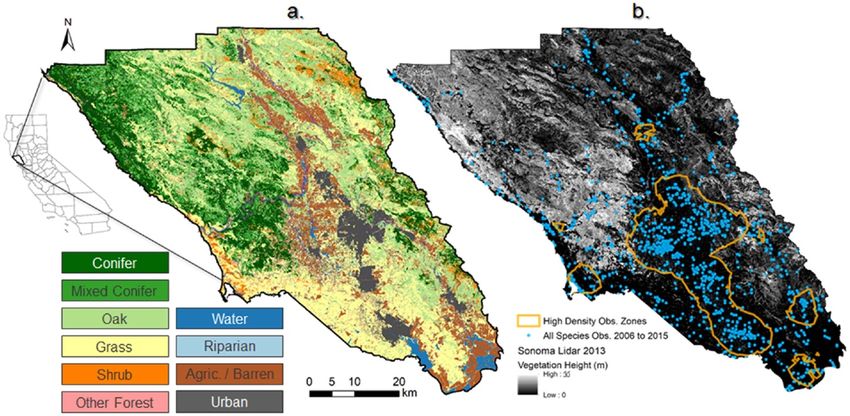
Environ. Res. Lett. 15 (2020) 095002                                                                      P Burns et al

and impacts at multiple ecosystem levels (Pereira et al     bioclimatic conditions (Wilson and Jetz 2016), or
2013, Corbane et al 2015, He et al 2015, Rocchini et al     land-cover classes (He et al 2015, Bradie and Leung
2015). Proenca and colleagues (2017) reviewed sci-          2017). When considering bird diversity, continental-
entific approaches to global biodiversity monitoring,       extent distributions are largely modeled with biocli-
with a focus on GEO BON’s Essential Biodiversity            matic variables (e.g. WorldClim; Fick and Hijmans
Variables, and highlight the use of remote sensing for      2017), which can predict overall physiological con-
characterizing ecosystem structure and function. In         straints, and correlate with broad vegetation patterns
terrestrial applications, remote sensors provide meas-      that influence habitat (Stralberg et al 2009, Lawler
urements of vegetation properties, including chem-          et al 2009). However, at regional extents and finer
istry, structure and phenology, which are related           spatial resolution (grain), information on vegeta-
to species habitat requirements, specifically shelter       tion structure is useful for characterizing micro-
and food resources. In this regard, many unexplored         habitats, particularly in areas with heterogeneous
opportunities with new technologies remain open to          vegetation patterns, for example from topographic
investigation. For example, NASA’s Global Ecosys-           variation (Stralberg et al 2009) or land-use/land-
tem Dynamics Investigation (GEDI; Dubayah et al             cover change (Sohl 2014). Bird species diversity is
2020) is a light detection and ranging (lidar) sensor       known to respond to both vegetation structure and
that was installed on the International Space Station       floristic diversity (Macarthur and Macarthur 1961,
(ISS) in December 2018. This sensor makes fine-scale        Rotenberry 1985, Adams and Matthews 2019), both
measurements of 3D vegetation structure, such as            factors that have been missing in models operating
overall canopy height and vertical distributions of         beyond the plot scale. Recent developments in air-
plant material. The acquisition of these structural         borne remote sensing have provided missing links
measurements over the majority of the land surface          at regional to local extents, implying possibilities for
is expected to lead to significant advances in biod-        broader-extent applications when these technologies
iversity monitoring and modeling (Bergen et al 2009,        are elevated to space.
Goetz et al 2014, Bakx et al 2019). In this study, our           Airborne lidar surveys of topography and veget-
primary goal is to examine the importance and added         ation structure are becoming more frequent, but are
value of 3D canopy structure data derived from sim-         still limited in areal extent due to operational costs.
ulated GEDI lidar waveforms in regional-extent bird         While most airborne lidar sensors typically capture
species distribution models (SDM).                          discrete returns from small footprints (20 m dia-
surveys and radar remote sensing suggests a drastic         meter) collected over a wider area (Lim et al 2003;
decline of 2.9 billion birds since 1970 (Rosenberg          Anderson et al 2016; Hancock et al 2019). Lidar
et al 2019). Similar to other taxa, habitat loss is a       data are already improving our understanding of how
major driver of reduction in bird species abundance         vegetation structure influences bird species distribu-
and range (Jetz et al 2007). Suitable bird habitat          tions at multiple spatial scales (Tattoni et al 2012,
includes necessities like food, water, shelter, and nest-   Rechsteiner et al 2017, Carrasco et al 2019) and sev-
ing sites. Habitats are characterized at various scales,    eral review papers have examined lidar-based stud-
from broad associations to more descriptive micro-          ies that consider avian distributions (Vierling et al
habitats. Habitat associations are typically related        2008, Davies and Asner 2014, Bakx et al 2019). In
to land-cover classes, frequently broad vegetation          general, current research tends to use airborne lidar
types (e.g. coniferous forest, grassland), which can be     and derived metrics related to canopy height, ver-
extracted from existing national or global land-cover       tical and horizontal variability, and cover, as well
maps (e.g. MODIS C6; Sulla-Menashe et al 2019).             as understory density. Most studies report a posit-
Habitat associations can be further subdivided into         ive effect of lidar metrics in explaining bird distribu-
microhabitats (e.g. shaded ground beneath mature            tions and/or patterns of richness, however the extent
canopy) which are characterized by fine-scale topo-         and scale of analysis are important factors. Species
graphy, climate, and vegetation structure. Measure-         sense and respond to a range of temporal and spatial
ments of vegetation structure are not widely available      scales (Wiens 1989, Levin 1992), and this has import-
at fine scales, but previous work suggests that struc-      ant implications for parameterizing and interpret-
tural complexity is associated with a greater variety of    ing SDMs. (Mayor 2009) and McGarigal et al (2016)
microhabitats which can lead to higher diversity and        review how hundreds of studies address the issue of
abundance due to more opportunities for foraging,           scale dependence, finding no consensus. At a min-
shelter, and nesting (Cody 1985, Hunter 1999, Whit-         imum, they recommend testing SDMs at a variety of
taker et al 2001, Hill et al 2004).                         spatial scales, ideally optimizing the scale of each vari-
     Previous SDM applications have mainly                  able (multi-scale optimization).
used remote sensing to derive spatially-explicit                 In this study, we focus on implementing simu-
environmental predictors, such as topography and            lated GEDI lidar—the first spaceborne lidar mission

                                               2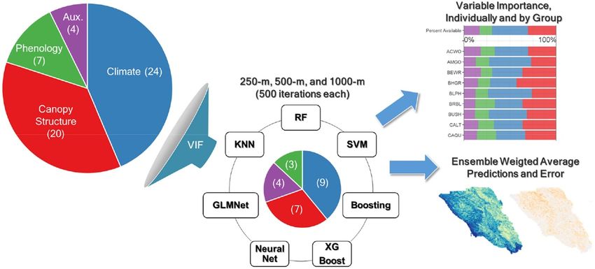
Environ. Res. Lett. 15 (2020) 095002                                                                   P Burns et al

designed specifically to measure vegetation struc-         2.2. Bird species data
ture. The instrument is scheduled to collect data for      2.2.1. Selecting species of interest
a minimum of two years, from 2019 to 2020. Ini-            We gathered field observations from point count sur-
tial GEDI data were released on January 22, 2020,          veys collected by Point Blue Conservation Science
and so our analysis uses 2 years of GEDI data sim-         (figure 1; appendix A) from the California Avian
ulated from airborne lidar data. Previous research         Data Center (http://data.prbo.org/cadc2/) between
using NASA’s airborne full waveform Land Veget-            2006 and 2015, along with data from the citizen sci-
ation and Ice Sensor (LVIS), a precursor to GEDI,          ence observation network eBird (Sullivan et al 2009),
showed that lidar metrics were useful for modeling         and the Breeding Bird Survey (Sauer et al 2017).
bird species richness, abundance, and habitat qual-        eBird data comprised the majority of records. We
ity at local extents (Goetz et al 2007, 2010). More        used data from all detailed survey events that recor-
recent research has used space-based ICESat-1 wave-        ded all species present, and thus from which we
form lidar at broader scales (Goetz et al 2014), corrob-   could discern detection or non-detection. If pres-
orating other studies showing vegetation properties        ence detections occurred in a given grid cell at a par-
derived from multispectral satellites (e.g. MODIS),        ticular resolution then that cell response was clas-
such as percent tree cover and life form type, along       sified as presence (value = 1). Grid cell surveys in
with bioclimatic variables were generally sufficient       which the observer did not encounter the species of
predictors of breeding bird species richness.              interest were classified as absence (value = 0). We
     We created SDMs for 25 species of birds in            selected the top 25 species based on number of grid
Sonoma County (figure 1) using canopy structure            cell presences at 250 m spatial resolution (see table
predictor variables as well as additional climate,         1). Main species habitat associations (Conifer, Oak,
phenology, and other auxiliary geospatial predictors.      Shrub, Riparian, Grass, Urban, and Variable; table 1)
Our three objectives are to: (1) generate bird SDMs        were determined from the Sonoma County Breeding
and determine the importance of individual pre-            Bird Atlas, Audubon Guide to North American Birds
dictor variables and variable groups for 25 bird spe-      (https://www.audubon.org/bird-guide) and The Cor-
cies; (2) determine whether including Canopy Struc-        nell Lab of Ornithology Birds of North America guide
ture variables improve SDM performance, while also         (https://birdsna.org; Rodewald 2015). A variable hab-
exploring the impacts of spatial scale; and, (3) map       itat association means that the species does not spend
probability of bird species occurrence and associated      a majority of time in a given habitat.
uncertainty of these predictions.
                                                           2.3. GEDI lidar and canopy structure predictor
                                                           variables
2. Methods
                                                           2.3.1. GEDI Instrument Description
                                                           The GEDI lidar sensor measures vertical canopy
2.1. Spatial and temporal domain of SDMs
                                                           structure of forests between ±51.6 degrees latitude.
We focus on Sonoma County because there are a rel-
                                                           The instrument emits pulses of energy (1064-nm)
atively large number of geolocated bird species obser-
                                                           which reflect off of various canopy layers and/or the
vations and the entire county is covered by airborne
                                                           Earth’s surface, and the returned energy of each pulse
lidar data (figure 1) which we used for the GEDI
                                                           is recorded as a short duration time series. Using the
simulation. A previous effort, the Sonoma County
                                                           speed of light, ISS orbital geometry, and precise posi-
Breeding Bird Atlas (U.S. Geological Survey 2019),
                                                           tioning, this time series is geolocated on the Earth’s
was based entirely on field observations and mapped
                                                           surface and transformed into a waveform—a pro-
occurrence of bird species in Sonoma County at 5-km
                                                           file of returned energy discretized into 15-cm vertical
spatial resolution. We sought to create finer spatial
                                                           height bins for each ∼22- to 25 m diameter footprint
resolution maps showing probability of occurrence
                                                           (Dubayah et al 2020). Footprints are separated by
by generating three regularly-spaced square grids cov-
                                                           approximately 60 m along each of the 8 ground tracks
ering the county at 250-, 500- and 1000 m spatial
                                                           and by 600 m between tracks. GEDI, like other lidar
resolution.
                                                           systems, is not able to make measurements through
    The airborne lidar collection occurred from
                                                           clouds.
September to November 2013 and is the primary
temporal constraint on our analysis. We chose water
years (starting in October and ending in Septem-           2.3.2. Canopy Structure predictor variables from
ber) 2013 to 2015 to bracket the lidar data collection.    simulated GEDI
Additional remote sensing datasets used for SDMs           The primary GEDI data product (L1B) is a geolocated
were temporally-aggregated to the entire three-year        lidar waveform. Variations of the main waveform and
period. Due to the limited spatial coverage of species     waveform-derived metrics (L2; Tang et al 2012) are
observations from this three-year period, we exten-        output for each footprint.
ded the species observation window to ten years                We simulated two years of GEDI lidar observa-
(2006 to 2015).                                            tions from airborne lidar data by using the methods

                                              3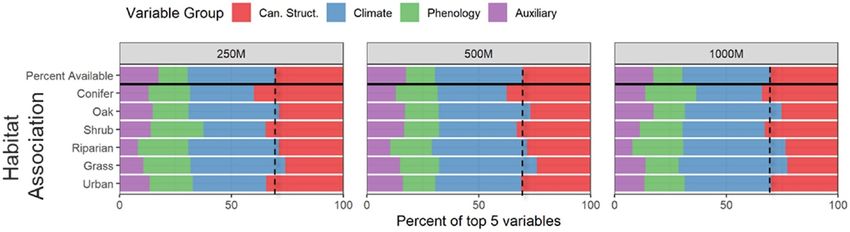
Environ. Res. Lett. 15 (2020) 095002                                                                                     P Burns et al

   Figure 1. Sonoma County, California, USA dominant vegetation and land cover classes (a.) and vegetation height map (b.)
   derived from airborne lidar survey in 2013 ( sonomavegmap.org ). All species observation locations from 2006 to 2015 (blue dots
   in b.) and corresponding high density observation areas (orange outlines in b.) are shown as well.

                           Table 1. Species selected for distribution modeling and their habitat association.

Species Code     Common Name                        Pres. Grid Cells at 250 m      Abs. Grid Cells at 250 m     Habitat Association

ACWO             Acorn Woodpecker                               189                            718              Oak
AMGO             American Goldfinch                             114                            486              Grass
BEWR             Bewick’s Wren                                  98                             615              Variable
BHGR             Black-headed Grosbeak                          106                            517              Variable
BLPH             Black Phoebe                                   193                            478              Riparian
BRBL             Brewer’s Blackbird                             172                            499              Urban
BUSH             Bushtit                                        165                            579              Oak
CALT             California Towhee                              306                            438              Shrub
CAQU             California Quail                               193                            520              Shrub
CBCH             Chestnut-backed Chickadee                      127                            544              Conifer
DEJU             Dark-eyed Junco                                155                            589              Conifer
HOFI             House Finch                                    261                            362              Urban
LEGO             Lesser Goldfinch                               164                            459              Grass
MODO             Mourning Dove                                  281                            741              Urban
NOFL             Northern Flicker                               89                             624              Conifer
NOMO             Northern Mockingbird                           214                            808              Oak
NUWO             Nuttall’s Woodpecker                           152                            471              Oak
OATI             Oak Titmouse                                   181                            490              Oak
RWBL             Red-winged Blackbird                           175                            448              Riparian
SOSP             Song Sparrow                                   213                            610              Riparian
SPTO             Spotted Towhee                                 137                            486              Conifer
STJA             Steller’s Jay                                  119                            625              Conifer
WCSP             White-crowned Sparrow                          168                            432              Shrub
WEBL             Western Bluebird                               132                            491              Grass
WESJ             Western Scrub-jay                              257                            414              Oak
                                       Mean                     174                            538
                               Std. Deviation                   57                             108

described by (Hancock et al 2019). All simulated                      generated the geostatistical model for each Canopy
L2 variables are based on a gaussian ground-finding                   Structure metric using the ArcGIS Pro Geostatist-
algorithm (Hofton et al 2000). The ‘Canopy Struc-                     ical Wizard and the ‘Simple’ Kriging method. We
ture’ predictor variables used in this study are                      resampled the 50 m prediction raster to our three
described in appendix Table C1. Since GEDI is a                       different analysis scales using an averaging method.
sampling instrument we used the ‘Moving Window                        Additional details regarding airborne lidar data pro-
Kriging’ tool from ArcGIS Pro to produce predicted                    cessing, GEDI simulation processing and interpola-
Canopy Structure metric values at 50 m intervals. We                  tion can be found in appendix C.a.

                                                      4
Environ. Res. Lett. 15 (2020) 095002 P Burns et al
2.4. Additional predictor variables Indices (DHI) Phenological predictor variables from
2.4.1. Climate. MODIS, most recently described by Hobi et al (2017)
We selected six ‘Climate’ predictor variables from the and Radeloff et al (2019). These indices are meas-
California Basin Characterization Model (BCM; Flint ures of vegetation productivity over the course of a
et al 2013) to include in SDM: precipitation (Ppt), year. We were limited to using MOD13 NDVI since
average minimum temperature (TMn), average max- it is the only index measured at (approximately) our
imum temperature (TMx), potential evapotranspir- finest analysis scale. The DHIs we calculated include:
ation (PET), actual evapotranspiration (AET), and (1) DHI sum—the area under the phenological curve
climatic water deficit (CWD). The monthly data for of a year, (2) DHI min—the minimum value of the
water years 2013, 2014 and 2015 were resampled from phenological curve of a year, (3) DHI var—the coef-
a native spatial resolution of 270 m to our three ana- ficient of variation of the phenological curve of a year,
lytical spatial scales using an averaging method. Vari- (4) DHI median—the median value of the composite
ables for each water year were then grouped and time series, (5) DHI 95p—the 95th percentile value
averaged into four three-month periods: October- of the composite time series, and (6) DHI seasonal
December (Q1), January-March (Q2), April-June difference—the difference between mean June and
(Q3), and July-September (Q4). Final SDM climate mean November NDVI, a potential proxy for decidu-
variables were averages of the three water years (2013– ousness in this area. The six DHI metrics were calcu-
2015) for each three-month BCM variable, resulting lated at their nominal spatial resolution (232-, 463-,
in 24 total ‘Climate’ variables for each spatial analysis 927 m) and then resampled to our analysis scales. See
scale. appendix C.c. for additional details.
2.4.2. Auxiliary variables 2.5. Species distribution model approach
We used four ‘Auxiliary’ predictor variables as inputs 2.5.1. Individual SDMs
to SDMs: elevation, distance to ocean coast, distance We combined Climate (24), Canopy Structure (20),
to streets, and distance to streams. Sonoma County Phenology (7), and Auxiliary (4) variables for a total
has a diverse topography, ranging from Pacific coast- of 55 predictors covering Sonoma County at each
lines to mountains greater than 1000 m in eleva- spatial resolution. We rescaled each predictor vari-
tion. Elevation can be a proximate determinant of able by subtracting the mean and dividing by the
a species’ presence (Hof et al 2012). Elevation ras- standard deviation. To account for potential multi-
ters were derived from the USGS National Elevation collinearity we used a variance inflation factor (VIF)
Dataset (NED; 1/3 arcsecond native spatial resolu- analysis to remove the most correlated variables. We
tion). In Sonoma County, distance to coast is cor- used our highest spatial scale scenario (250 m) vari-
related with a longitudinal pattern of habitats. Closer able values and set a VIF threshold value greater
to the coast are mixed hardwood and conifer forests, than or equal to 10—equivalent to excluding vari-
such as Coastal redwoods and Douglas fir, with inter- ables that have an R-square of 0.9 or higher when
spersed patches of chaparral, and further inland occur regressed against all other variables. We selected the
conifer patches, oak woodlands, chaparral and grass- same variables for the other two model scales that use
lands. Distance to coast was also calculated initially as Canopy Structure predictors. This model scenario is
a 30 m raster from a coastal vector layer using Arc- referred to as ‘All with Canopy Structure’. For com-
GIS. Distance to streets was incorporated as a proxy parison we ran a scenario referred to as ‘All without
gradient for human influence. We used the Sonoma Canopy Structure’ which excluded Canopy Structure
County streets vector layer to calculate distances in a variables.
30 m raster. Distances to streams were incorporated as We ran seven individual SDMs (Random Forests,
an additional predictor related to moisture and water Support Vector Machine, Boosting, Extreme Gradi-
availability. Numerous species of birds prefer habit- ent Boosting, Neural Network, Net Regularized Gen-
ats along or near streams (Rottenborn 1999, Mcclure eralized Linear Models, and K-Nearest Neighbors)
et al 2015). We used the lidar-derived streams vector 500 times (bootstraps) for each species, resolution,
layer from the Sonoma County Vegetation Mapping and model scenario combination. Each bootstrap
and Lidar program (https://sonomavegmap.org) to corresponded to a random sample (80% training,
calculate distances in a 30 m raster. All auxili- 20% testing) of spatially-thinned species observations
ary variables were resampled to the spatial analysis (Aiello-Lammens 2015) and associated predictor
scales (250-, 500-, and 1000 m) using an averaging variables. Cross-validation was used to tune models
method. and prevent overfitting. Additional details related to
individual model tuning and bootstrapping can be
2.4.3. Phenology found in appendix D. We focused on the area under
Multispectral satellites like the Moderate Resolution the receiver operator characteristic curve (AUC;
Imaging Spectroradiometer (MODIS) are particu- Fielding and Bell 1997) for individual model evalu-
larly useful for monitoring vegetation presence, vital- ation. AUC values equal to 0.5 mean that the pre-
ity, and phenology. We calculated Dynamic Habitat dicted values are equivalent to random guesses. AUC
5Environ. Res. Lett. 15 (2020) 095002 P Burns et al
values greater than 0.5 and up to 1 (perfect) indicate models do not over-fit when tested with and without
that the model has some level of predictive power. a variable, as they may include variable interactions
that increase model complexity and may not correctly
2.5.2. Variable importance reflect the ecology of the species (Aguirre-Gutiérrez
We used a sensitivity analysis method from the et al 2013, Bell and Schlaepfer 2016). This was noted
R package rminer (Cortez and Embrechts 2013, by (Araujo and Guisan 2006), who recommend the
Cortez 2016) to assess variable importance. We use of carefully chosen predictors (see also Araújo et al
selected the data-based sensitivity analysis (DSA) 2019). We postulated that GEDI variables provide
method and associated average absolute deviation ecologically-meaningful information about vegeta-
from the median (AAD) for measuring importance. tion structural complexity that partly determines the
We focused on the model scenario ‘All with Canopy niche of several of our study species. We visually com-
Structure’ and assessed variable importance for spe- pared the performance of SDMs that included and
cies both in terms of individual variables and vari- omitted Canopy Structure variables. We expected the
able groups (Climate, Canopy Structure, Phenology, algorithms used would adjust model complexity to
and Auxiliary). We also assessed variable importance optimally predict with and without the Canopy Struc-
aggregated by habitat association. ture variables. However, we also expected Canopy
Structure variable importance would still be evident
2.5.3. Ensemble SDMs as an increase in performance when they are included
We generated two different types of ensembles, an in the model.
individual iteration ensemble (IIE) and combined Though information from the full range of the
iteration ensemble (CIE). The IIE for each species species has been noted as very important for SDM
calculates a weighted average prediction (Marmion performance (Kadmon et al 2003, Syphard and
et al 2009) value from up to seven individual model Franklin 2010, Martínez-Freiría et al 2016; see review
predictions for a single bootstrap (figure 2). To cre- in Engler et al 2017), the geographic coverage of
ate this ensemble we only selected individual mod- the airborne lidar dataset precluded us from run-
els with AUC greater than 0.5 and then calculated ning models outside Sonoma County. Relatively less
a weighted average prediction for each grid cell, important than geographic bias and sample size
where the weights were based on adjusted AUC (Thibaud et al 2014), spatial autocorrelation will also
(AUC score minus 0.5). All prediction averaging affect SDM performance and was not included in
was done following a logit transform of the model our models. Since our goal was to evaluate the rel-
predictions. Averaged values were then transformed ative importance of the Canopy Structure variables
back to probability (0 to 1). Our second ensemble in SDMs, we focused on building relatively accurate
method, CIE, aggregates species model predictions models and comparing among constructs that vary
from individual models across all 500 bootstraps, only with respect to the variables used.
again weighting the final prediction value by adjus-
ted AUC. The maximum number of individual pre- 2.6.2. Logistic regression analyses
diction values was 3500 (7 models ∗ 500 iterations), In order to provide additional evidence of the impact
assuming all individual models had AUC greater than of Canopy Structure variables, we used all the vari-
0.5. We used the weighted average prediction value ables remaining after VIF to construct an additive
and associated weighted standard error to display logistic regression model (the ‘All with Canopy Struc-
probability of occurrence and associated uncertainty ture’ model scenario), and also fitted the ‘All without
for each species (figure 2). All SDM analyses were Canopy Structure’ model scenario. For each boot-
performed in R (R Core Team 2019). Appendix H strap sample, we then calculated the likelihood ratio
lists specific R packages used and associated test statistic of the full model vs the restricted model
references. (i.e. with vs without Canopy Structure), and report
the range of values of the statistic in relation to the
2.6. Impact of Canopy Structure variables on value at which it is expected to occur fewer than 5%
model performance of the times (the ‘statistically significant’ departure
2.6.1. Ensemble SDMs value). Results of this logistic regression analysis are
Differences in predictive accuracy when contrast- provided for comparison in appendix E.c. since our
ing model constructs can be highly informative with main focus is the use of Canopy Structure variables
respect to the importance of a particular predictor for in ensemble SDMs.
understanding the niche of a species, and for man-
agement and decision-making (Austin and Van Niel 3. Results
2011 Mod et al 2016, Bell and Schlaepfer 2016). How-
ever, consistency in identification of important envir- 3.1. Predictor variables and importance
onmental variables varies with the algorithm used The VIF method used to remove highly-correlated
and other factors, so caution must be taken to ensure predictor variables at 250 m spatial resolution
6Environ. Res. Lett. 15 (2020) 095002 P Burns et al
Figure 2. Overview of SDM framework for the ‘All with Canopy Structure’ modelling scenario. VIF reduced the total number of
predictor variables to 23. Then for each of the 25 species we used seven different machine learning algorithms at three different
spatial scales. We ran 500 bootstraps for each species and scale. We calculated the aggregated variable importance for each species
and also produced weighted prediction and uncertainty maps.
reduced the number of predictor variables from 55 and habitat associations, Climate variables most fre-
to 23. This reduction left 38% of Climate, 35% of quently ranked in the top-5, but the relative frequen-
Canopy Structure, 100% of Auxiliary and 43% of cies generally matched the proportion of Climate
Phenology predictor variables. The following Cli- variables available relative to the total number of vari-
mate variables remained: Actual Evapotranspira- ables. However, Oak, Riparian, and Grass specialists
tion (AET) from Q1, Q2, Q3, and Q4, Potential had a higher frequency of Climate variables ranked
Evapotranspiration (PET) from Q1 and Q2, Pre- in the top-5. For all habitat associations, Phenology
cipitation from Q1 (PptQ1), Maximum Temperat- variables ranked in the top-5 more frequently than
ure from Q1 (TMxQ1), and Minimum Temperature would be expected based on proportion of Phenology
from Q1 (TMnQ1). The following Canopy Struc- variables available relative to the total number of vari-
ture variables remained: Biomass (BM; referred to ables. Across all habitat associations at 250 m, Auxili-
as BM_2_1 in appendix Table C1), Leaf Area Index ary variables comprised 12.9% of the top-5 (vs. 17.4%
0- to 10 m, 10- to 20 m, 20- to 30 m, and 30- to expected), Phenology 19.3% (vs. 13.0% expected),
40 m, Vertical Distribution Ratio Middle (VDRM) Canopy Structure 32.5% (vs. 30.4% expected), and
and Vertical Distribution Ratio Bottom (VDRB). All Climate 35.3% (vs. 39.1% expected). These import-
Auxiliary variables remained after VIF. The follow- ance patterns are corroborated by another perspective
ing Phenology variables remained: NDVI Annual in which we summed total importance for each res-
95th Percentile (NDVI_Ann_95p), NDVI Seasonal olution and predictor variable group (supplementary
Difference (NDVI_Seas_Diff), and NDVI Variance figure E2 (stacks.iop.org/ERL/15/095002/mmedia)).
(NDVI_Var). The correlation matrix for the remain- The DSA importance method also provided
ing variables is shown in appendix figure C3 . insight into which individual predictor variables were
For all 500 bootstraps we summarized variable most important (appendix figure E3). Individual
importance by predictor variable group for hab- Phenology variables were relatively more important
itat associations (figure 3) and individual species than median importance of variables from all mod-
(appendix E). We ranked DSA variable importance els, regardless of habitat association. Canopy Struc-
for each individual bootstrap and then selected the ture variables were usually about as important as
top-5 most important variables from each boot- the median variable importance. The two vertical
strap. Figure 3 shows the relative distribution of all distribution ratios (VDRB and VDRM) were more
top-5 variables by variable group and habitat asso- important than other canopy structure variables, with
ciation. From this perspective at 250 m, Canopy VDRB showing noticeably higher relative importance
Structure variables most frequently ranked in the for all habitat associations. Canopy Structure vari-
top-5 most important variables for Conifer, Shrub, ables BM, LAI 0- to 10 m, and LAI 10- to 20 m
and Urban specialists. The importance of Canopy were relatively more important for Conifer special-
Structure diminishes at coarser spatial resolutions, ists, particularly at finer spatial resolution. Climate
such that Climate variables most frequently ranked variables were relatively homogenous in their import-
in the top-5 when considering Shrub and Urban ance, but TMxQ1 showed noticeable deviation from
specialists at 1000 m. Across all spatial resolutions the median importance value. Precipitation from the
7Environ. Res. Lett. 15 (2020) 095002 P Burns et al
Figure 3. The percent of time that individual variables from different groups were included in the top-5 most important (DSA
method) variables across all 500 bootstrap iterations. Percent Available is percentage of variables available from a group (Canopy
Structure, Climate, Phenology, Auxiliary) relative to the total number of variables remaining after VIF (n = 23) and can be
thought of as a baseline for comparison if all variables were equally important. The dashed vertical line corresponds to Canopy
Structure percent available and is used for assessing the relative importance of this variable group for different habitat
associations. We included all models (except XGBoost) which had AUC > 0.5 and used at least 5 variables.
first quarter (PptQ1) was another relatively import- 3.2.2. Influence of spatial resolution
ant Climate variable. Importance of Climate variables We summarize ‘All with Canopy Structure’ median
generally increased going from fine- to coarse-scale. model performance by spatial resolution in Supple-
mentary Table F2. Considering all 25 SDMs, most
(11) have the highest median AUC value at 250 m.
Grass and Riparian habitat specialists are notable
3.2. Model performance exceptions, with all of their highest median AUC
3.2.1. Comparing performance of different model values at 500 m and 1000 m, respectively. Conifer,
scenarios Oak, and Shrub specialists generally have the highest
Ensemble models were most frequently the best per- median AUC at 250 m spatial resolution. Supple-
forming models over all bootstraps (appendix F.a.). mentary Table F2 also shows the difference between
Figure 4 shows notched boxplots corresponding to the maximum and minimum AUC medians across
Ensemble Weighted Average (EWA) AUC values from all spatial resolutions, providing insight into the scale
500 bootstraps for each species and resolution. These variability of each SDM. The average scale variab-
boxplots are useful for visualizing differences among ility is 0.03 AUC, while the maximum variability is
bootstrap population medians. The ‘All with Canopy 0.067 AUC. Therefore, the effect of scale on median
Structure’ scenario showed median AUC improve- model performance is similar to the effect of incor-
ments (i.e. non-overlapping notches) for at least one porating Canopy Structure variables.
resolution for 19 species: CBCH (all), DEJU (250- and
500 m), NOFL (250- and 500 m), SPTO (250- and
500 m), STJA (all), AMGO (250- and 500 m), BUSH 3.3. Ensemble maps
(250 m), NOMO (500 m), NUWO (250- and 500 m), We calculated CIE weighted average predictions from
OATI (250 m), WESJ (250 m), RWBL (500 m), SOSP individual models which had AUC values greater than
(250 m), CALT (all), CAQU (250 m), WCSP (500 m), 0.5. Figure 5 shows species distribution maps for birds
BRBL (all), BEWR (250- and 500 m), and BHGR from a range of habitat associations as predicted by
(250 m). Every Conifer specialist showed a median the ensemble weighted average as well as the cor-
AUC improvement for at least one spatial resolution. responding uncertainty. The uncertainty estimates
Five of the six Oak specialists showed an improve- include variance due to the model used, the bootstrap
ment in performance for at least one spatial resolu- sampling, and unexplained variance by the model.
tion. Few of the Grass or Riparian specialists showed Because of the small sample sizes of the bird observa-
improvement after incorporating Canopy Structure tion data, the total predicted error is relatively large.
variables. All three Shrub specialists showed a median All species maps are presented in appendix G.
AUC improvement for at least one spatial resolution.
Lastly, two of four Urban species showed a median 4. Discussion
AUC improvement for at least one spatial resolution.
Thresholded differences in AUC are shown in Supple- Our ability to describe, parameterize, and model spe-
mentary Table F1. For example, at 250 m, the median cies’ habitat continues to improve with the addi-
AUC value increased by at least 0.02 AUC for 10 of 25 tion and refinement of relevant geospatial datasets.
species, while the 95th percentile AUC value increased Our central objective was to determine the added
for 14 of 25 species. The maximum increase in median benefit of Canopy Structure variables from simu-
AUC after incorporating Canopy Structure variables lated GEDI lidar in SDMs that also include relev-
was 0.04 for CBCH. ant Climate, Phenology, and Auxiliary variables. We
8Environ. Res. Lett. 15 (2020) 095002 P Burns et al
Figure 4. Model performance comparison between two model scenarios—‘All with Canopy Structure’ vs. ‘All without Canopy
Structure’. Each boxplot corresponds to EWA AUC values from up to 500 bootstraps. Notches that do not overlap can be
interpreted as having different median values. ‘X’ points on each boxplot correspond to the 95th percentile value.
quantified the added benefit of these Canopy Struc- formance. For this analysis we selected three prac-
ture variables by calculating variable importance of tical SDM spatial scales which coincided with readily
the ‘All with Canopy Structure’ model scenario and available and ecologically-meaningful Climate, Phen-
by comparing the performance of this model scen- ology, and Auxiliary predictor variables. Below we
ario against the ‘All without Canopy Structure’ model discuss the variables that remained after the VIF pro-
scenario using 500 bootstraps. The spatial scale at cess, their importance, the change in SDM perform-
which SDMs are generated is a very important consid- ance after incorporating Canopy Structure variables,
eration and impacts our estimates of variable import- current constraints on the analysis, and ideas for
ance and comparative assessment of model per- building on this work in the future.
9Environ. Res. Lett. 15 (2020) 095002 P Burns et al
Figure 5. Ensemble maps of weighted average probability of occurrence and associated uncertainty of the mean for one species
from each habitat association at 250 m spatial resolution. Uncertainty of the mean prediction is shown as the range of the
standard error confidence interval, that is the upper 1 SE confidence interval minus the lower 1 SE confidence interval. Other
maps are presented in Supplementary Material Appendix G.
10Environ. Res. Lett. 15 (2020) 095002 P Burns et al
4.1. Model variables and importance for perching or nesting. Some species SDMs may find
Methods to reduce redundant information across this variable useful for discriminating between can-
predictor variables, such as VIF, are useful for creating opy structure characteristics. For instance, this was
models that are parsimonious and interpretable one of the most important variables for California
in terms of variable importance. Furthermore, the Towhee, which commonly uses dense shrub/scrub
elimination of certain variables can provide insight areas that are low to the ground.
regarding unique information content relative to the Canopy Structure variables were most important
entire stack of environmental predictors. Considering for Conifer specialists (figure 3), suggesting that these
all variable groups, we found Climate variables to be species seem to prefer locations with certain Can-
the most important overall. Maximum temperature opy Structure characteristics (i.e. based on import-
was the most important Climate variable for Grass ance metrics, more biomass at the canopy level and
and Oak species, which agrees with previous stud- denser foliage, or LAI, in the 0- to 10 m and 10- to
ies (Howard et al 2015, Bradie and Leung 2017). Six 20 m strata). This agrees with our observations of
of nine Climate variables were associated with either these conifer-associated species in Sonoma County.
potential or actual evapotranspiration (ET), which For example, Dark-eyed Junco is often found in
is related to a combination of temperature, mois- areas with complex vegetation structure less than
ture availability, and plant productivity. Hawkins et al 5 m from the ground, but also forages in mid-
(2003) and Coops et al (2018) found ET variables to canopy. During the breeding season, males often
be important for predicting species richness at broad sing from exposed perches near the tops of con-
spatial scales. Barbet-Massin and Jetz (2014) showed ifers and snags. Chestnut-backed Chickadee prefers
that annual PET was among the most relevant vari- structurally-complex mature conifer forests, as cor-
ables for predicting bird species distributions in the roborated by the importance of the variable LAI 20-
conterminous U.S. The ET variables do not appear to to 30 m, and is often found gleaning small insects and
be relatively as important when grouped by habitat other arthropods from bark and twigs.
association, but still contain some unique informa- Phenology variables mainly capture temporal
tion. For example, PETQ2 is one of the most import- cycling of top-of-canopy foliage status, but in some
ant variables for Bushtit and Mourning Dove. cases (low to moderate forest cover) may contain
Seven Canopy Structure variables remained fol- information about foliage density associated with the
lowing VIF reduction, and as a group were usually the near-infrared component of NDVI which is related to
second most important variable group depending on the phenomenon of leaf additive reflectance (Jensen
habitat association. Canopy structure is an import- 1996). The Phenology variables had the highest top-
ant determinant of avian diversity, including the par- 5 importance difference relative to their expected
titioning of niches for species coexistence, changes importance (+6.3% overall at 250 m) suggesting that
in microclimate (Zellweger et al 2019) and refuge these variables contain particularly useful informa-
from predation (Davies and Asner 2014). Müller et al tion for bird SDMs. Visually, the three Phenology
(2010) found that 3D structure measured with air- variables show some correspondence with broad land
borne lidar was the main statistical determinant of cover and vegetation classes (figure 2), which may
bird assemblages in a German temperate mixed forest. provide sufficient predictive information for some
Macarthur and Macarthur (1961) first reported the SDMs. Canopy Structure variables from GEDI also
link between bird species diversity and foliage height had a positive top-5 importance difference (+2.1%
diversity (FHD). However, neither version of the overall at 250 m) for all habitat associations. Can-
FHD metrics remained following VIF reduction. This opy Structure variables likely complement Climate
is not necessarily because the variable is without util- and Phenology variables by adding 3D information
ity, but rather some of its information content varied related to microhabitat structure that is not captured
linearly with other variables that also include inform- by the other variables we used. This 3D perspective
ation about the vertical distribution of plants, like has the greatest benefit for Conifer specialists (+9.5%
vertical distribution ratios (VDRB and VDRM), LAI overall at 250 m).
profiles, and NDVI. VDRB was a particularly import-
ant variable for all habitat associations. This variable 4.2. SDM performance
was initially included to characterize how evenly plant 4.2.1. Ensemble model performance perspective
material is distributed, as it compares the overall can- Fewer than half of the ensemble SDMs had median
opy height to the height of 50% of the cumulative AUC greater than 0.7, a threshold for assessing SDM
waveform signal. In theory, values close to 0.5 indic- quality (Pearce and Ferrier 2000, Duan et al 2014).
ate an even distribution, while lower values should The overall performance of these 25 SDMs was
indicate a higher concentration of plant material in likely related to the bird observation data and the
the understory, and vice versa. In actuality, when large distribution range of the individual species
examining the kriged raster we observe that the vari- (Mcpherson and Jetz 2007). Although Sonoma
able shows spatial correspondence with tall vegetation County is relatively diverse in terms of climate, topo-
or built-up structures, both of which could be useful graphy, and vegetation type, more bird observations
11Environ. Res. Lett. 15 (2020) 095002 P Burns et al
spanning a wider range of the environmental pre- incorporation of Canopy Structure variables less fre-
dictor variables could lead to better presence/absence quently improved model performance. Mertes and
separation and thus improved SDM performance. Jetz (2018) found resampling environmental pre-
Furthermore, the best performing SDMs were gener- dictor variables with fine spatial structure decreased
ally associated with Conifer and Oak species, which the performance of SDMs. Curry et al (2018) found
are relatively more selective and less likely to occur that spatially-explicit ensemble models with finer-
across multiple habitats in Sonoma County. Fairly scale predictor variables consistently performed bet-
common species SDMs, such as Mourning Doves, ter at predicting occurrence for 3 of 11 grassland bird
Song Sparrows, and House Finches did not benefit species. Our results, and those from others, are related
much from the incorporation of Canopy Structure to the spatial structure and autocorrelation of Canopy
information due to their high prevalence in multiple Structure variables (Mertes and Jetz 2018). We did not
habitats (Kadmon et al 2003, Brotons et al 2004, but explicitly factor in spatial autocorrelation of environ-
see Gavish et al 2017 for a counter-example). mental predictor variables into SDMs, but semivari-
Larger observation datasets and more certainty ograms generated for each Canopy Structure vari-
in presence/absence records both help models to able confirmed the spatial structure (semivariogram
more accurately depict the niche of common species range) of each variable was generally within 250-
(Kadmon et al 2003). While there are a large num- to 1000 m (Supplementary Table C2). The major-
ber of survey events in Sonoma County (n = 10606), ity of semivariograms generated from GEDI simu-
these occurred largely in the same locations—when lation subsets within Conifer and Oak forests have
aggregated within cells, only a few hundred cells were ranges below 500 m. Additional SDM performance
surveyed (see table 1). However, because most cells improvements may be possible through exploration
had many survey events, our determination of pres- of multi-scale optimization (e.g. Wan et al 2017,
ence/absence within each cell is probably very accur- Stevens and Conway 2019), especially when consider-
ate, the more so for these common and easy to identify ing even finer-scale vertical (Seavy et al 2009, Gastón
generalist species. It is therefore likely that the rel- et al 2017) and horizontal (Huang et al 2014, Carrasco
atively poor performance of most models is due to et al 2019) Canopy Structure variables.
low sample sizes and associated lack of high-density
observations from different land-cover classes. These
are common limitations associated with citizen sci- 4.3. Constraints on the current analysis
ence observations, such as those used in this study The primary limitations of this study are the quant-
(Boakes et al 2010, Beck et al 2014). ity and geographic distribution of bird observations,
Although Canopy Structure variables frequently as well as our ability to represent canopy structure at
improved median model performance, especially at optimal scales using simulated spaceborne lidar data.
finer spatial resolution, the improvement in perform- The biggest limitation associated with the bird spe-
ance was relatively modest considering the number of cies observation data is a lack of high-density, evenly-
new variables (and potential amount of new inform- distributed spatial observations. As shown in figure 1,
ation) added to the models. The various machine most observations occurred in urban/suburban areas.
learning models used in the ensemble performed Since we are primarily interested in how forest Can-
well at discerning patterns and optimizing predic- opy Structure variables improve SDMs, this was not
tions with relatively few predictor variables. Another the ideal network of observations because relatively
reason for modest improvements in performance few observations were distant from roads and inside
was related to correlation and information-overlap of intact forests. The impact of these Canopy Struc-
between variables remaining following VIF. Even ture variables is likely more difficult to resolve when
after using VIF, there was still correlation among the urban features are mixed with tree canopies at the grid
predictor variables (see appendix figure C3) suggest- cell resolutions used in this analysis. We would expect
ing that some canopy structure information could be to receive a more consistent signal from a ‘natural’
explained by other variables. For examples we found forest canopy compared with a suburban or urban-
Pearson correlation coefficients greater than 0.6 when wildland interface canopy interspersed with built-up
regressing NDVI95p against three Canopy Structure structures.
variables (Biomass, LAI 0- to 10 m, and LAI 10- to Other limitations are associated with our ability
20 m). to represent canopy structure using simulated space-
Lastly, spatial scale dependence cannot be ignored borne lidar data. First, the simulated lidar data are
in SDM analyses (Wiens 1989, Jackson and Fahrig hypothetical geospatial observations—actual mission
2015). In this study, we found an average scale footprint locations will vary as a function of orbital
variability of 0.03 AUC (Supplementary Table F2) geometry, which cannot be predicted exactly, and
which is similar to the effect of incorporating Canopy local cloud cover patterns. Another major limitation
Structure variables in some SDMs. When going concerns interpolation from footprints (L2 products)
from fine to coarse spatial scale, we found Can- to grids (L3 products). There are numerous options
opy Structure variable importance decreased and for interpolating point data to continuous grids
12Environ. Res. Lett. 15 (2020) 095002 P Burns et al
depending on the nature of the dataset. As a start- simultaneously from ICESat-2, may have some util-
ing point, we used a kriging methodology similar to ity in filling GEDI canopy structure coverage gaps.
the one outlined in the GEDI L3 Algorithm Theoret- The Advanced Topographic Laser Altimeter System
ical Basis Document (Dubayah et al 2020). Over the (ATLAS) instrument on-board ICESat-2 uses photon
course of two years, GEDI is expected to provide suf- counting technology which has limitations in dense
ficient coverage for generating L3 products at 1000 m vegetation, especially during daytime observations
spatial resolution. However, coverage gaps will still be (Popescu et al 2018). Although vegetation measure-
present in 1000 m spatial resolution grids and would ment is not the primary focus of the ICESat-2 mis-
be even more prevalent at the finer spatial resolu- sion, we still expect some useful canopy structure
tions used in this study (see appendix figure C2). observations in forests of sparse to moderate canopy
For natural and continuous forest types, we expect cover (Neuenschwander and Pitts 2019).
this kriging method to be a good option for inter-
polation as neighboring grid cells tend to have sim- 5. Conclusions
ilar geostatistical characteristics. For fragmented or
urban/suburban forests, this method may not be as We incorporated Canopy Structure variables derived
effective. More advanced interpolation methods such from simulated GEDI lidar into 25 bird SDMs in
as co-kriging (Tsui et al 2013) or fusion (Swatantran Sonoma County, CA. We found Canopy Structure
et al 2012) with auxiliary data with continuous spatial variables were generally the second most important
coverage, like Sentinel-1, Sentinel-2 or Landsat satel- group of variables across a variety of habitats. Canopy
lite imagery, may prove to be better options for inter- Structure was most important for Conifer and Shrub
polating large areas or filling in sparsely-sampled grid habitat associations. The incorporation of Canopy
cells. Structure variables into ensemble SDMs resulted in
performance improvements for the majority of spe-
4.4. Future directions cies across all spatial analysis resolutions. More SDMs
We expect canopy structure measurements from showed higher, albeit modest, performance improve-
GEDI will be informative for modelling habitat for ments at the finest spatial analysis scale suggesting
a variety of forest-dependent taxa. Our modeling that Canopy Structure variables are more beneficial
approach is applicable to larger spatial extents and at smaller scales which are more in line with micro-
taxa, but one important consideration would be the habitats. Although this study covers a regional spatial
source of Climate data, as BCM is a California- extent and limited number of species, it demonstrates
wide climate product with an unusually fine spatial that Canopy Structure variables derived from space-
resolution (270 m). Global climate variables from borne lidar have the potential to improve our ability
WorldClim (Fick and Hijmans 2017), which have to map species distributions.
approximately 1000 m spatial resolution, are more Our understanding of global forest canopy struc-
commonly used for larger SDM extents outside of ture will grow by orders of magnitude over the
the conterminous U.S. We note that this resolution next decade as a result of the GEDI and ICESat-
matches the planned GEDI L3 products. It will be 2 spaceborne lidar missions. We encourage future
necessary to test the utility of these global climate SDM efforts to explore the utility of operational
variables and GEDI L3 metrics in SDMs at their native lidar products from these sensors across natural and
resolution. However, for some species the tradeoff in anthropogenic landscapes. Future SDM studies may
model performance as a function of spatial scale may also benefit from fusion of spaceborne lidar with
preclude the use of relatively coarse vegetation struc- other remote sensing data as this combination can
ture and/or climate data (Manzoor et al 2018). Altern- provide more continuous spatial coverage across a
atively, shifting to more of a microhabitat focus, broader range of spatial scales. SDMs generated at
recent studies have proposed frameworks for dynam- even finer spatial scales may benefit more from lidar-
ically modeling microclimate using fine-scale topo- derived Canopy Structure variables, resulting in more
graphy and vegetation structure datasets derived from detailed map products for land management and con-
remote sensing (Kearney et al 2019, Lembrechts et al servation of species habitat.
2019). Using these finer spatial and temporal scale cli-
mate datasets in conjunction with vegetation struc- Acknowledgments
ture measurements will improve our understanding
of the mechanistic interplay between the two, as well Airborne lidar data were provided by the University of
as how species and ecosystems respond to changes in Maryland and the Sonoma County Vegetation Map-
climate (Zellweger et al 2019). ping and Lidar Program under grant NNX13AP69G
It will also be beneficial to explore data and from NASA’s Carbon Monitoring System (Dubayah,
methods for increasing the quantity and coverage of PI). We acknowledge Curt Joyce at Quantum Spatial
canopy structure measurements. GEDI is scheduled Inc. who helped to acquire the airborne lidar data.
for two years of data collection on the ISS but a dif- Curt, a leader in outdoor, remote sensing, and envir-
ferent type of spaceborne lidar data, being collected onmental communities, passed away in 2014. Xiaoli
13You can also read