Measurements and quality control of ammonia eddy covariance fluxes: a new strategy for high-frequency attenuation correction - Atmos. Meas. Tech
←
→
Page content transcription
If your browser does not render page correctly, please read the page content below
Atmos. Meas. Tech., 12, 6059–6078, 2019
https://doi.org/10.5194/amt-12-6059-2019
© Author(s) 2019. This work is distributed under
the Creative Commons Attribution 4.0 License.
Measurements and quality control of ammonia eddy covariance
fluxes: a new strategy for high-frequency attenuation correction
Alexander Moravek1,a , Saumya Singh1 , Elizabeth Pattey2 , Luc Pelletier2 , and Jennifer G. Murphy1
1 Department of Chemistry, University of Toronto, Toronto, ON M5S 3H6, Canada
2 Agricultureand Agri-Food Canada, Ottawa, ON K1A 0C6, Canada
a now at: Department of Chemistry, York University, Toronto, ON M3J 1P3, Canada
Correspondence: Alexander Moravek (amoravek@yorku.ca)
Received: 9 May 2019 – Discussion started: 18 June 2019
Revised: 11 September 2019 – Accepted: 19 September 2019 – Published: 21 November 2019
Abstract. Measurements of the surface–atmosphere ex- pose a new method that simulates the flux loss by using the
change of ammonia (NH3 ) are necessary to study the emis- analyser time response that is determined frequently over the
sion and deposition processes of NH3 from managed and nat- course of the measurement campaign. A correction that uses
ural ecosystems. The eddy covariance technique, which is the as a function of the horizontal wind speed and the time re-
most direct method for trace gas exchange measurements at sponse is formulated which accounts for surface ageing and
the ecosystem level, requires trace gas detection at a fast sam- contamination over the course of the experiment. Using this
ple frequency and high precision. In the past, the major lim- method, the median flux loss was calculated to be 46 %,
itation for measuring NH3 eddy covariance fluxes has been which was substantially higher than with the ogive method.
the slow time response of NH3 measurements due to NH3
adsorption on instrument surfaces. While high-frequency at-
tenuation correction methods are used, large uncertainties in
these corrections still exist, which are mainly due to the lack Copyright statement. ©Crown copyright 2019. Distributed under
of understanding of the processes that govern the time re- the Creative Commons Attribution 4.0 License.
sponse. We measured NH3 fluxes over a corn crop field us-
ing a quantum cascade laser spectrometer (QCL) that en-
ables measurements of NH3 at a 10 Hz measurement fre-
quency. The 5-month measurement period covered a large 1 Introduction
range of environmental conditions that included both periods
of NH3 emission and deposition and allowed us to investigate Knowledge of ammonia (NH3 ) exchange processes between
the time response controlling parameters under field condi- ecosystems and the atmosphere is essential for improving our
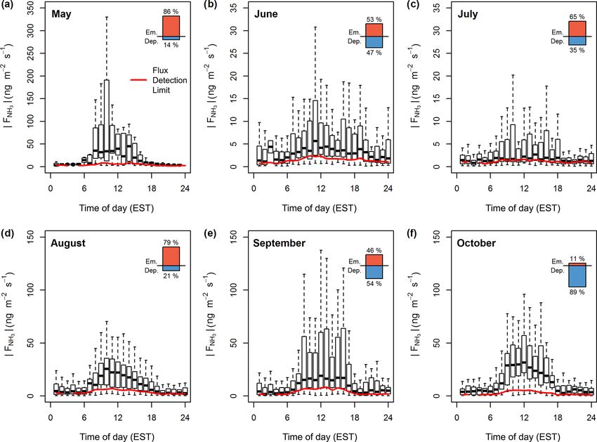
tions. Without high-frequency loss correction, the median understanding of its impact on air quality, global warming
daytime NH3 flux was 8.59 ng m−2 s−1 during emission and and ecosystem health. As the most abundant base in the at-
−19.87 ng m−2 s−1 during deposition periods, with a median mosphere, NH3 is responsible for the formation of ammo-
daytime random flux error of 1.61 ng m−2 s−1 . The overall nium aerosol, impairing air quality and affecting climate. For
median flux detection limit was 2.15 ng m−2 s−1 , leading to example, it is estimated that 34 % of fine particulate matter
only 11.6 % of valid flux data below the detection limit. From in Europe is directly linked to emission of NH3 that gener-
the flux attenuation analysis, we determined a median flux ates secondary particulate matter (Pozzer et al., 2017). Am-
loss of 17 % using the ogive method. No correlations of the monium aerosol is often found to be the dominant particu-
flux loss with environmental or analyser parameters (such as late matter component in areas with strong ammonia sources,
humidity or inlet ageing) were found, which was attributed as was recently reported for North China and the Great Salt
to the uncertainties in the ogive method. Therefore, we pro- Lake region (Li et al., 2019; Moravek et al., 2019). Further-
more, deposition of NH3 has been shown to strongly im-
Published by Copernicus Publications on behalf of the European Geosciences Union.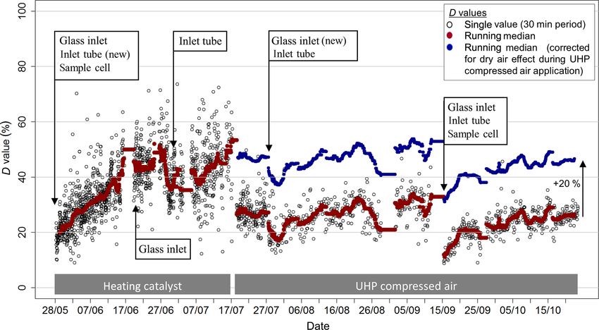
6060                            A. Moravek et al.: Measurements and quality control of ammonia eddy covariance fluxes

pact low-nitrogen ecosystems, thereby reducing biodiversity       cally cooled lasers. A greater laser stability and output power
(Erisman et al., 2013).                                           is given by quantum cascade lasers (QCL) which can be
   Major sources of NH3 to the atmosphere are emissions           Peltier-cooled (McManus et al., 2010). Ferrara et al. (2012,
from agriculture, with 24 Tg yr−1 from livestock and live-        2016) and Whitehead et al. (2008) used pulsed QCL spec-
stock waste and 9.4 Tg yr−1 from synthetic fertiliser appli-      trometers for NH3 eddy covariance measurements on agri-
cations on agricultural fields being emitted globally (Paulot     cultural sites, whereas Zöll et al. (2016) employed a more
et al., 2014). In urban environments, fossil-fuel based NH3       sensitive continuous-wave QCL instrument to measure NH3
emissions can be the dominant source (Pan et al., 2016). The      fluxes above a peatland.
understanding and quantification of these emission sources           The common limitation of the previous studies using fast-
is critical to propose effective NH3 control and mitigation       response NH3 analysers is the instrument time response due
strategies. However, to date large uncertainties exist regard-    to the surface adsorption of NH3 . It is well-known that ad-
ing the magnitude of NH3 emissions. This is in part due to        sorption and desorption of NH3 to and from surfaces, includ-
difficulties and challenges in measuring NH3 fluxes, espe-        ing inlet tubing, can be significant. This effect slows the time
cially in environments where NH3 fluxes are small and/or          response of the measuring system leading to high-frequency
frequent changes between net emission and deposition are          attenuation (HFA) of the measured NH3 time series, which
expected.                                                         affects the NH3 flux measurements by eddy covariance. To
   To measure NH3 exchange at the ecosystem level, mi-            avoid these effects, Sun et al. (2015) employed a custom-built
crometeorological methods including gradient, relaxed eddy        open-path QCL (Miller et al., 2014) to measure eddy covari-
accumulation (REA) and eddy covariance (EC) have been             ance fluxes above a cattle feedlot. While open-path QCL sys-
used in the past. The method used largely depends on the          tems have the advantage of avoiding HFA effects, they may
expected flux magnitude, the site layout and the available in-    introduce flow distortion due to their size when placed close
strumentation. Systems based on the capture of NH3 by de-         to the sonic anemometer and require frequent cleaning of the
nuders or the thermal conversion to nitric oxide (NO) have        exposed cell mirrors (Sun et al., 2015). As closed-path sys-
been employed for flux gradient (e.g. Famulari et al., 2010;      tems will still play an important role in the future, our study
Flechard and Fowler, 1998; Sutton et al., 2000; Walker et al.,    focuses on the performance and quality control of closed-
2006; Wolff et al., 2010) and REA-based flux measurements         path eddy covariance systems. The magnitude of flux loss
(Baum and Ham, 2009; Hansen et al., 2013, 2015; Hensen            due to HFA in closed-path systems is highly variable depend-
et al., 2009; Myles et al., 2007; Nelson et al., 2017; Zhu et     ing on the instrumental set-up and meteorological conditions.
al., 2000). The success of both methods often relies on the       For past NH3 eddy covariance field measurements, the esti-
precise and accurate determination of a concentration differ-     mated flux loss ranged between 20 % and 50 % (Ferrara et al.,
ence measured over a typical time period of 30 min up to          2012, 2016; Sintermann et al., 2011; Whitehead et al., 2008;
several hours. Especially under conditions where the mea-         Zöll et al., 2016). Although the flux loss can be corrected for
sured vertical concentration gradient is small, like for flux     in post-processing using spectral correction techniques, the
measurements above forests, the REA method is the much            applied correction factor can vary significantly depending on
stronger approach. The flux gradient measurement heights          the chosen correction method (Ferrara et al., 2012). A lack of
and the size of the REA deadband largely impact the concen-       understanding of the factors impacting the time response of
tration difference, and their choice has to be considered care-   NH3 eddy covariance systems is responsible for this uncer-
fully in the flux measurement set-up and operation (Moravek       tainty.
et al., 2014).                                                       From previous studies, it is known that adsorption and des-
   The eddy covariance method is the most direct method           orption of NH3 is governed by the surface area and mate-
of quantifying ecosystem-scale turbulent fluxes as it relies      rial of the inlets and internal instrument components, with
on the covariance between the near-ground turbulence and          stainless steel showing significantly slower time responses
the scalar of interest. For this, the scalar has to be mea-       than polyethylene (PE) or polytetrafluoroethylene (PTFE)
sured at a fast time response (≤ 0.1 s) with concurrent ad-       (Whitehead et al., 2008). Ellis et al. (2010) showed that heat-
equately high precision. In the last 2 decades, the develop-      ing of their perfluoroalkoxy (PFA) inlet tubing to 40 ◦ C for
ment and improvement of mass spectrometry and infrared            NH3 mixing ratios above 30 ppbv reduced the HFA signif-
spectroscopy techniques for fast measurements of NH3 pro-         icantly, whereas Sintermann et al. (2011) found that heat-
vided the opportunity to measure NH3 fluxes using eddy co-        ing their drift tube inlet to 180 ◦ C enabled a time resolu-
variance. Shaw et al. (1998) presented the first eddy covari-     tion high enough for eddy covariance measurements. It is
ance measurements of NH3 using a tandem mass spectrome-           suspected that heating removes – at least partially – liquid
ter, and Sintermann et al. (2011) employed a proton transfer      and molecular water layers on the surface, which decreases
reaction mass spectrometer to measure NH3 emissions after         the adsorption sites for the polar NH3 molecule (Sintermann
slurry application. For laser-based eddy covariance measure-      et al., 2011), although NH3 can also interact directly with
ments, Famulari et al. (2004) and Whitehead et al. (2008)         the surface material. Roscioli et al. (2015) showed that us-
utilised diode laser absorption spectroscopy using cryogeni-      ing active passivation by continuously adding a fluorinated

Atmos. Meas. Tech., 12, 6059–6078, 2019                                             www.atmos-meas-tech.net/12/6059/2019/
A. Moravek et al.: Measurements and quality control of ammonia eddy covariance fluxes                                        6061

amine into the sample gas improved the time response sig-           on environmental and operational conditions. Currently, con-
nificantly, as the polar amine group of the molecule occupies       tinuous wave QCL spectrometers are the most precise high
potential NH3 adsorption sites and NH3 does not react with          time resolution NH3 measurement systems available; how-
its non-polar fluoro chain. Still, there is a lack of compre-       ever, their operation under field conditions requires careful
hensive mechanistic understanding of NH3 sorption on sur-           set up and regular maintenance. With our findings we pro-
faces (Sintermann et al., 2011), which is needed to reduce          vide details on the set-up and operation of the QCL which
the uncertainties of the HFA correction for NH3 eddy covari-        are helpful for investigators that aim to use it for eddy co-
ance fluxes. There is evidence that adsorption and desorp-          variance NH3 flux measurements in the future.
tion processes act at different rates (Whitehead et al., 2008),
which would skew the high-frequency NH3 distribution and
may impact the flux covariance calculation. While Ellis et          2     Methods
al. (2010) found the time response to degrade with the rel-
ative humidity of ambient air, the potential effect on NH3          2.1     Flux measurements
fluxes is not accounted for in the currently used HFA flux
correction methods (Ferrara et al., 2012; Zöll et al., 2016).       2.1.1    NH3 detection with QCL
Evidence that the time response is improved when the NH3
mixing ratio changes are larger (Ellis et al., 2010) can be in-     A quantum cascade tunable infrared laser differential absorp-
terpreted in two ways: fluxes with higher magnitudes need to        tion spectrometer (QC-TILDAS, Aerodyne Research Inc.,
be corrected less than small fluxes, or fluxes at higher ambi-      USA) was used to measure the NH3 mixing ratio at a 10 Hz
ent concentrations are less attenuated due to a higher passiva-     sampling frequency for eddy covariance flux measurements.
tion of the surface. Finally, the time response effect of surface   The QC-TILDAS (referred to as QCL hereafter) retrieves
ageing and surface deposition of particulate matter is poorly       the NH3 absorption spectrum at 967.3 cm−1 using a thermo-
understood and accounted for in HFA correction methods              electrically cooled continuous wave quantum cascade laser
(Roscioli et al., 2015; Sintermann et al., 2011; Whitehead et       (Alpes Lasers, Switzerland), which is scanned across the full
al., 2008). As our understanding of the NH3 time response in        NH3 transition within the spectral window. A continuous
changing environmental and instrumental conditions is lim-          wave laser has an increased power output over a pulsed laser,
ited, the analysis of flux datasets under a wider range of con-     which was used in the version of the QCL described in de-
ditions than previously sampled are needed reduce the uncer-        tail by Ellis et al. (2010), and is therefore more suitable for
tainties in the HFA correction of NH3 fluxes.                       the high precision measurements needed for the eddy covari-
   In this study, we employed a NH3 eddy covariance system          ance method. As illustrated in Fig. 1, the laser beam is di-
over an entire growing season from May to October 2017 at           rected into an astigmatic Herriot multiple pass absorption cell
a corn field in Eastern Canada. The system used a closed-           (0.5 L, 76 m effective pass length) coated with a hydropho-
path continuous wave QCL spectrometer with a 5.5 m heated           bic coating to reduce the interaction of NH3 with cell walls.
PFA inlet line. The objectives were to (1) limit adsorp-            To minimise line-width broadening of the absorption peak,
tion/desorption of NH3 in the inlet of the QCL, and (2) quan-       the pressure in the absorption cell is kept at approximately
tify its impact on the systems time response under a large          4.67 kPa. A reference cell containing ethylene (C2 H4 ), a less
range of environmental and instrumental conditions in order         surface reactive gas that contains an absorption line near that
to obtain a deeper understanding of the processes that gov-         of NH3 , is used for absorption line lock. The signal and
ern the time response and of how this is ultimately applied         reference paths are focused on the same thermoelectrically
to the NH3 flux correction. This includes, for example, the         cooled mercury–cadmium–telluride (HgCdTe) infrared de-
examination of the relationship between time response and           tector (Vigo Systems, Poland).
humidity or the flux magnitude. Due to the 5-month measure-            The laser control, spectral retrieval and mixing ratio cal-
ment period, we are able to examine the effect of inlet ageing      culations are managed by the TDLWintel software pack-
and the benefit of cleaning procedures on the NH3 flux mea-         age (Aerodyne Research Inc., USA) described in Nelson
surement. Based on our findings, we present an approach to          et al. (2004). The measured NH3 spectrum is fitted at the
correct NH3 fluxes that uses our improved understanding of          10 Hz sample frequency by convolving the laser line shape
NH3 time response. The approach may also be used for flux           with a calculated absorption line shape based on the HI-
correction of other species that show a strong surface adsorp-      TRAN (high-resolution transmission) molecular absorption
tion, such as nitric or organic acids.                              database and the measured pressure, temperature and path
   Next to the issue of HFA, NH3 measurement systems need           length of the optical cell (Herndon et al., 2007). The soft-
to resolve small NH3 mixing ratio fluctuations at high time         ware allows for automatic user-defined additions of zero air
resolution. Especially under low flux conditions, a precise         via the use of a solenoid valve.
and stable operation of the NH3 measurement system is re-              Variations in pressure, temperature and other disturbances
quired. For this reason, the paper also discusses the precision     may significantly impact the instrument performance by in-
and flux detection limit of the QCL spectrometer depending          fluencing the absorption spectrum fringe pattern. Fringes are

www.atmos-meas-tech.net/12/6059/2019/                                                Atmos. Meas. Tech., 12, 6059–6078, 2019
6062                                 A. Moravek et al.: Measurements and quality control of ammonia eddy covariance fluxes

Figure 1. Schematic overview of the measurement set-up. The glass inlet of the QCL is mounted next to the sonic anemometer (measurement
height 2.5 m, later 4.5 m). Inside the glass inlet (see Ellis et al., 2010), a critical orifice reduces the pressure regime and a sharp turn of the flow
path leads to a reduction of particulate matter. Heated sample tubing (length of 5.5 m) leads the sample air (flow rate of 13.4 to 15.4 L min−1 )
to the QCL, which is housed in a temperature and humidity controlled enclosure. Dotted lines show the electrical connections for data
acquisition and control of the inlet heating and QCL analyser.

structures in the absorption spectrum that are caused by op-                   measured using a closed-path infrared gas analyser (LI-7000,
tical interferences within the laser beam path and can be re-                  LI-COR, USA). The AAFC in-house data acquisition and
sponsible for signal drift if their pattern changes over time.                 control system, called “REAsampl” (Pattey et al., 1996), was
Especially for species that are typically present in the atmo-                 used to record the analogue channels of the various instru-
sphere in the lower parts per billion or parts per trillion mix-               ments at 20 Hz. The REAsampl software adjusts the prede-
ing ratio range, such as NH3 , the impact of fringes to the                    termined lags between the various close-path analysers and
absorption peak range can be significant. For that reason, the                 the vertical wind velocity, and rotates the horizontally sym-
operation of the QCL requires a stable environment to house                    metrical sonic anemometer head in the mean horizontal wind
the QCL and frequent background measurements with zero                         direction every hour when the hourly mean horizontal wind
air to account for potential drifts in the background spectrum.                velocity is greater than 1.5 m s−1 . During the few seconds of
                                                                               the rotation for aligning the anemometer, the raw data are
2.1.2    Set-up and operation of NH3 flux measurements                         not recorded. By aligning the anemometer, the flow distor-
                                                                               tion and lateral loss of covariance are minimised.
Eddy covariance flux measurements of NH3 were performed                           As shown in Fig. 1, the set-up of the QCL consisted of
from 28 May to 23 October 2017 on an agricultural corn                         five major parts: (1) the inlet system, (2) the QCL and chiller
field, equipped with twin flux towers near Ottawa in East-                     unit, (3) the valve and heating control box as well as en-
ern Canada (see Fig. 7, Pattey et al., 2006). The experimen-                   closure housing, (4) the vacuum pump and (5) the zero air
tal site is located on the premises of the Canadian Food In-                   source. The inlet was mounted at the mid-vertical distance
spection Agency (CFIA) and is managed by Agriculture and                       of the sonic anemometer open-path and 25 cm behind the
Agri-Food Canada (AAFC). Prior to the measurements, the                        anemometer open-path to minimise flow distortion from the
agricultural field was tilled and fertilised on 25 May using                   inlet on the wind velocity measurements and lateral loss of
granular urea fertiliser (155 kg N ha−1 ). The corn crop was                   covariance. The QCL uses a 10 cm quartz inlet which acts as
seeded on 28 May. The QCL was installed on the west eddy                       virtual impactor to remove particulate matter from the sam-
covariance flux tower, which had a fetch of 200 to 500 m de-                   ple air. As described in more detail in Ellis et al. (2010),
pending on the wind direction.                                                 about 90 % of the sample air makes a sharp turn (Fig. 1) and
   To measure the 3-D wind vector for the covariance cal-                      is pulled through the absorption cell, while 10 % of the flow,
culation, a CSAT3 (Campbell Scientific Inc, USA) sonic                         including particles larger than 300 nm due to their higher in-
anemometer was installed on the tower at 2.5 m above ground                    ertia, is pulled directly to the vacuum pump (TriScroll 600,
level (a.g.l.). To accommodate the growing corn canopy, the                    Agilent, USA). To limit the condensation of water and the
tower was raised to a measurement height of 4.5 m a.g.l. on                    interaction of NH3 with inlet surfaces, the glass inlet was
6 July. Water vapour (H2 O) and carbon dioxide (CO2 ) were                     internally coated with a hydrophobic fluorinated silane coat-

Atmos. Meas. Tech., 12, 6059–6078, 2019                                                             www.atmos-meas-tech.net/12/6059/2019/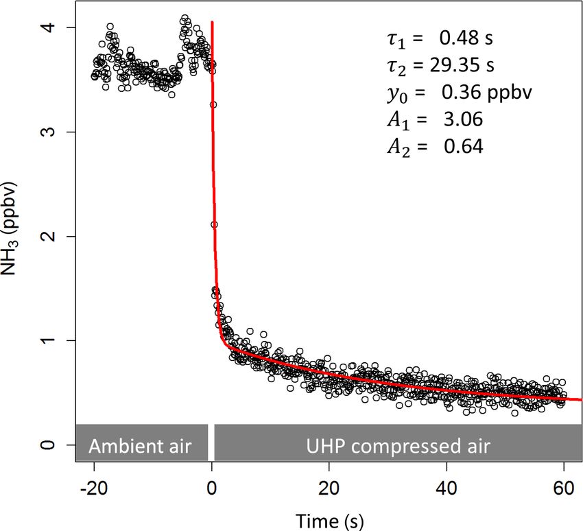
A. Moravek et al.: Measurements and quality control of ammonia eddy covariance fluxes                                        6063

ing and was heated constantly to 40 ◦ C. The glass inlet acts      pressed air consumption, the automated background interval
as a critical orifice that regulates the volume flow at the in-    was set to 1 h with a reduced duration of 3 min from 17 to
let. From 28 May to 27 July a glass inlet with a flow rate of      27 July. From 28 July to 31 August, the interval was set to 3 h
15.4 L min−1 was used, and after that period a glass inlet with    without significantly compromising the data quality. In the fi-
a flow rate of 13.4 L min−1 , which had a newly applied silane     nal phase of the measurement period, from 15 September to
coating, was utilised. For closed-path eddy covariance mea-        23 October, the background interval was set to 2 h. While the
surements, a high volume flow rate is essential to keep a plug     heating catalyst was running continuously, the zero air gas
flow in the inlet system, in order to minimise HFA in the in-      flow was introduced into the inlet by triggering a solenoid
let system. Depending on the flow rate and the actual sample       valve installed in the valve and heating control box.
gas temperature, the Reynolds number ranged between 3000              To test the effect of surface ageing on the time response
and 3700, indicating mainly transitional flow conditions with      and to reduce the interaction of NH3 with surfaces, regular
turbulent flow in the centre and laminar flow near the tubing      cleaning of the glass inlet, inlet line and the absorption cell
walls. The glass inlet was connected to the QCL via a 5.5 m        was performed by rinsing with deionised water and ethanol,
long 3/800 PFA sample tube, which was insulated and con-           while the tubing was heated to about 80 ◦ C during the clean-
trolled to 40 ◦ C. While raising the tower on 6 July, the QCL      ing process. The cleaning of the glass inlet was performed
was also raised by 2 m using wood pallets to keep a constant       on 22 June, 27 July and 12 September. The inlet tubing was
5.5 m sample tube length.                                          cleaned on 27 June, 27 July and 12 September. Along with
   The QCL, located at the bottom of the flux tower,               cleaning of the glass inlet and the inlet tubing, the inner sur-
was housed in an insulated aluminium enclosure that was            face of the absorption cell was also cleaned on 12 September.
equipped with two Peltier coolers to precisely control the
internal temperature of the box to 28.0 (±0.2) ◦ C. Next to        2.2   Eddy covariance flux calculation
the QCL, the enclosure also housed the chiller (Oasis Three,
Solid State Cooling Systems, USA) that was required for            The processing of the NH3 data leading to the final calcu-
stable temperature control of the infrared laser and the op-       lated NH3 fluxes consisted of four major steps: (1) process-
tical and electronic parts of the QCL. To prevent the build-up     ing and quality control (QC) of the digital NH3 mixing ratio
of heat inside the enclosure, the intake and exhaust vents of      data, (2) time synchronisation between the quality-controlled
the chiller were connected to the outside of the enclosure. A      digital NH3 data and vertical wind velocity data recorded us-
dehumidifier was built in to prevent condensation inside the       ing REAsampl, (3) flux calculation and (4) flux random error
box.                                                               calculation. The processing of QCL NH3 data as well as all
   The time series of the 10 Hz NH3 mixing ratios and anal-        other processing was performed using the R software pack-
yser parameters were digitally recorded on the QCL com-            age (R Core Team, 2017).
puter. For precise time synchronisation between the post-             The NH3 mixing ratio time series were first scanned for
processed digital NH3 mixing ratios and the vertical wind          periods of instrument failures and maintenance, which were
velocity, an analogue signal of the NH3 mixing ratio was           removed. Spike detection and removal was conducted using
recorded using REAsampl. A remote monitor was placed in            a running-mean low-pass filter. Spikes were identified best
a nearby trailer for regular checks and other operations like      as data points that exceeded 3.5 times the standard deviation
data transfer and manual valve switching, to avoid opening         of a 21-point averaging window. To correct for a potential
the temperature-controlled enclosure. Data were collected          drift of the QCL between two automated background periods
from the QCL computer regularly (every 2–4 d) and plotted          (varying from 30 min to 3 h), the background mixing ratios
for routine quality checks. To ensure optimal operation of the     were linearly interpolated between two consecutive back-
QCL instrumentation over the 5-month measurement period,           ground measurements and subtracted from the NH3 mixing
the status of the QCL was checked regularly via remote ac-         ratios. Following analogue acquisition using REAsampl, the
cess using a mobile hotspot.                                       20 Hz CSAT3 sonic anemometer and uncorrected NH3 data
   Zero air for frequent background measurements was in-           were extracted from the REAsampl raw data binary files, in
troduced at the front of the QCL glass inlet, which was de-        which the data associated with tower rotation were already
signed so that zero air encountered the inlet in the same way      removed.
as ambient air (Fig. 1). For zero air, a heating catalyst (Aadco      The time synchronisation between the NH3 mixing ra-
Instruments, USA) was used, which scrubs NH3 from ambi-            tios and vertical wind speed, which is essential for the eddy
ent air by catalytic thermal conversion at 300 ◦ C using pal-      covariance flux calculation, was performed in two steps:
ladium beads. The automatic background schedule was set            (1) time synchronisation between the digital NH3 data and
to flush the inlet with zero air for 5 min at the end of every     the REAsampl data and (2) time synchronisation between
30 min period from 28 May to 16 July. Due to an operation          the digital NH3 data and the vertical wind velocity. For the
failure of the heating catalyst, on 17 July the zero air source    former, a circular cross-correlation was performed between
was replaced by ultra-high purity (UHP) compressed zero air        the digital and analogue NH3 signals. Accounting for the
(Praxair Canada Inc., Canada). To minimise the UHP com-            analogue output delay, the time lag between both systems

www.atmos-meas-tech.net/12/6059/2019/                                                Atmos. Meas. Tech., 12, 6059–6078, 2019
6064                            A. Moravek et al.: Measurements and quality control of ammonia eddy covariance fluxes

was then determined as the position of the maximum corre-         calculated NH3 fluxes as they were incorporated as part of
lation. In the second step, a circular cross-correlation (us-     the high-frequency loss analysis discussed later in this paper.
ing a ±5 s window) between the time-synchronised sonic               The TK3 software package (Mauder and Foken, 2011) was
anemometer data and the digital NH3 data was used to ac-          used to calculate fluxes of momentum, sensible heat and la-
count for delays caused by the inlet system and the horizon-      tent heat, and NH3 flux quality parameters. The quality flag
tal displacement of the CSAT3 and the glass inlet. As the         scheme of Foken and Wichura (1996) was used to filter for
cross-correlation method between the vertical wind velocity       periods of low stationarity and low developed turbulence.
and a scalar only works well when turbulent fluxes are large      Furthermore, the TK3 program derives the random flux er-
enough, a quality assessment was performed on the results         rors of the NH3 flux. The random errors include (1) the errors
of the cross-correlation. Only lag times which were less than     due to the stochastic nature of turbulence and (2) the random
±2.5 s and had a cross-correlation value greater than 0.05        errors due to instrumental noise (Mauder et al., 2013). The
were used. Missing lag times were then replaced by the last       former is calculated in TK3 following the method of Finkel-
previous valid lag time. To detect further outliers, lag times    stein and Sims (2001), which calculates the variance of the
that were offset by more than ±1.5 s were set to the preceding    covariance function as a combination of the auto-covariance
lag time if the difference between the preceding and succes-      and cross-covariance terms with changing lag time. The ran-
sive lag time was less than 0.5 s, indicating a spike and not a   dom flux error due to instrumental noise is calculated in TK3
real shift in the lag time. After applying the described qual-    by extrapolating the auto-correlation function of the NH3
ity control, the standard deviation of the lag time was 1.1 s,    time series towards a zero lag time (Mauder et al., 2013).
which can be partly attributed to changes in the wind speed       As the random error calculation in TK3 was not success-
influencing the lag time between the sonic anemometer and         ful for all 30 min periods, we additionally determined the
inlet position.                                                   instrumental noise error (σcovnoise ) using the variance of the

   Background on the final eddy covariance flux calculation       zero air source measurements (conducted every 30 min to 3 h
and the required correction methods is well-documented in         throughout the experiment) as the variance of the NH3 mix-
the literature (Aubinet et al., 2012; Pattey et al., 2006). In    ing ratio and by implementing that in the instrumental noise
brief, NH3 fluxes are calculated by the covariance of the NH3     function used in Mauder et al. (2013). To be comparable to
mixing ratio (χNH3 ) and the vertical wind velocity (w) mul-      other NH3 flux studies, we also applied the approach used by
tiplied by the molar density of air (ρm ) as follows:             Sintermann et al. (2011), where the random flux error is de-
                                                                  termined for each 30 min period by the standard deviation of
                0
FNH3 = ρm · w0 χNH   ,                                     (1)                                stoch ) when using a time lag rang-
                                                                  the covariance function (σcov
                   3
                                                                  ing between −120 and −70 s and +70 and +120 s. Using
where χNH 0   and w0 denote the fluctuations of NH3 mixing                                                                   stoch .
                                                                  this approach, we defined the flux detection limit as 2·σcov
            3
ratio and the vertical wind velocity from their 30 min mean
value respectively. The NH3 fluxes presented in this study        2.3   Time response determination of NH3
are given in nanograms of NH3 per square metre per second               measurements
(ng NH3 m−2 s−1 ). Prior to the eddy covariance flux calcu-
lation, the 3-D wind vector coordinate is typically rotated to    A fast time response of the NH3 measuring system is essen-
ensure zero vertical wind velocity over the averaging period      tial for performing eddy covariance measurements. To un-
(Finnigan et al., 2003; Wilczak et al., 2001). Due to the tower   derstand the processes that impact the adsorption and des-
rotation mechanism used in this study, the wind vector was        orption of NH3 to the measurement system, knowledge of
already rotated into the mean wind direction. Variations in       the system’s NH3 time response is important. The time re-
the air density caused by temperature and air moisture fluctu-    sponse of the QCL NH3 measurements is mainly determined
ations may impact the eddy covariance flux and are typically      by two processes (Whitehead et al., 2008): (1) the exchange
corrected for by the WPL correction (Webb et al., 1980).          of the sample air volume in the inlet line and the sample cell
The sensible heat flux-induced fluctuations of the ambient        and (2) the adsorption and desorption of NH3 at the inlet
air temperature are expected to be efficiently damped by the      and sample cell walls. As a result, the time response can be
heat exchange in the inlet system and the 5 m long heated in-     described by a double exponential function giving two time
let line. An effect of air moisture fluctuations caused by the    constants, τ1 and τ2 , representing the time response towards
latent heat flux on the NH3 flux is possible, although it was     the exchange of the sample air volume and wall interactions
found that the effect on NH3 fluxes is negligible (≤ 1 %) due     respectively:
to the relatively low concentrations of NH3 in ambient air
(Ferrara et al., 2016; Pattey et al., 1992). For these reasons,
the WPL correction was not applied for the NH3 fluxes in                                  −(t − t0 )
                                                                  f (t) = y0 + A1 · exp
this study. High-frequency loss corrections, like for the flux                                 τ1

loss due to the distance between the CSAT3 and the QCL                               −(t − t0 )
glass inlet (Moore, 1986), were not applied to the initially            + A2 · exp                ,                             (2)
                                                                                        τ2

Atmos. Meas. Tech., 12, 6059–6078, 2019                                              www.atmos-meas-tech.net/12/6059/2019/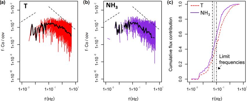
A. Moravek et al.: Measurements and quality control of ammonia eddy covariance fluxes 6065
as no adequate description of the surface adsorption and des-
orption processes currently exists. Experimental approaches
typically compare the co-spectrum of the vertical wind ve-
locity and the attenuated scalar time series to the co-spectrum
of a non-attenuated reference flux. The sensible heat flux is
most often used as a reference flux, either from direct mea-
surements or from parameterisation available in the literature
(Kaimal and Finnigan, 1994). In this study we used the ogive
method described in Ammann et al. (2006). The ogive of a
scalar flux (Ogws ) is calculated by the cumulative integral of
the co-spectrum (Cows ) as
Z ∞
Ogws (f ) = Cows (f ) df (4)
1/t
over the observed frequency range, beginning with the low-
est frequency (1/t, where t is the averaging interval). If the
ogive is normalised by the covariance, the ogive value at the
highest frequency is 1. The flux loss is derived by scaling the
normalised ogive of the scalar flux to the normalised ogive
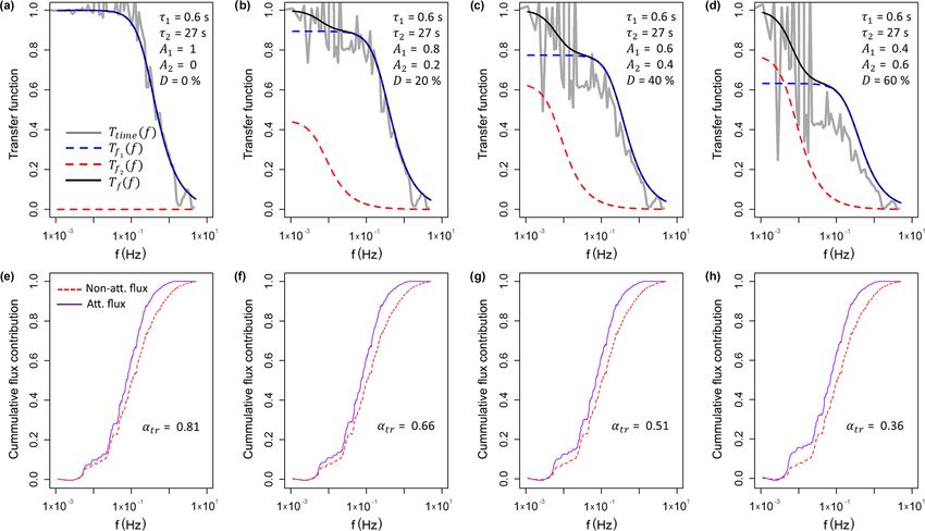
Figure 2. Time response of the 10 Hz NH3 measurement. Shown
of the sensible heat flux at a given limit frequency (f0 ). The
is the step change NH3 mixing ratios after switching from ambient
air to the UHP compressed air. The red line is the fit of the double scalar ogive value at the highest frequency then represents
exponential decay function. the flux attenuation factor (between 0 and 1). The limit fre-
quency is defined as the highest frequency at which no HFA
occurs and can be determined by comparing the scalar co-
where t0 is the start time and y0 is the offset from zero spectrum to the sensible heat flux co-spectrum.
(Fig. 2); A1 and A2 are proportionality coefficients that ac- Ideally, a reference scalar is used that shows the highest
count for the contribution of each process to the overall time scalar similarity to the investigated flux. The water vapour
response. Accordingly, the percentage contribution of the flux is expected to have a similar sink and source distribu-
wall interaction processes can be described as follows (El- tion to NH3 , but the measured flux may experience high-
lis et al., 2010): frequency loss if measured with a closed-path analyser.
Therefore, in this study we used the measured non-attenuated
A2
D= · 100 %. (3) sensible heat flux as a reference.
A1 + A2
Along with the time constants τ1 and τ2 , D can be used to 2.4.2 Time response method
evaluate the performance of the QCL system with respect
Another approach to correct for the HFA is to simulate the
to its time response. To determine the time response for our
flux loss by knowing the flux loss transfer function, which
instrument set-up, the double exponential function (Eq. 2)
represents the flux attenuation factor as a function of fre-
was fitted to the step change in the NH3 mixing ratios when
quency. The transfer function can be obtained by applying
switching from ambient air to zero air measurements as part
a low-pass filter, which represents the HFA of the system,
of the automated background correction. Those fits were per-
to the time series or flux of a non-attenuated scalar and then
formed for each background period in order to obtain the
comparing the filtered and non-filtered fluxes. In this study,
temporal variation of the time response over the course of
we determined the transfer function through the system’s
the entire measurement period.
time response, which was determined over the entire mea-
2.4 Analysis of flux loss due to high-frequency surement period as described in Sect. 2.3. As for the ogive
attenuation method, we used the sensible heat flux as a reference flux.
A low pass-filter can be applied either (1) in the frequency
2.4.1 Ogive method domain or (2) in the time domain. For the former method,
a transfer function is applied to the sensible heat flux co-
The attenuation of the high-frequency scalar time series due spectrum, which we modified using both τ1 and τ1 from
to a slow response leads to an underestimation of the calcu- Eq. (2). However, the low-pass filter effect of the inlet tub-
lated eddy covariance flux. Both theoretical and experimental ing introduces a phase shift next to the attenuation of high-
approaches are used to quantify the flux loss and ultimately frequency amplitudes (Horst, 1997; Massman and Ibrom,
correct for it; a summary is given in Foken et al. (2012). 2008). For that reason, we applied a low-pass filter in the
For NH3 the HFA needs to be determined experimentally, time domain to the high-frequency temperature time series.
www.atmos-meas-tech.net/12/6059/2019/ Atmos. Meas. Tech., 12, 6059–6078, 2019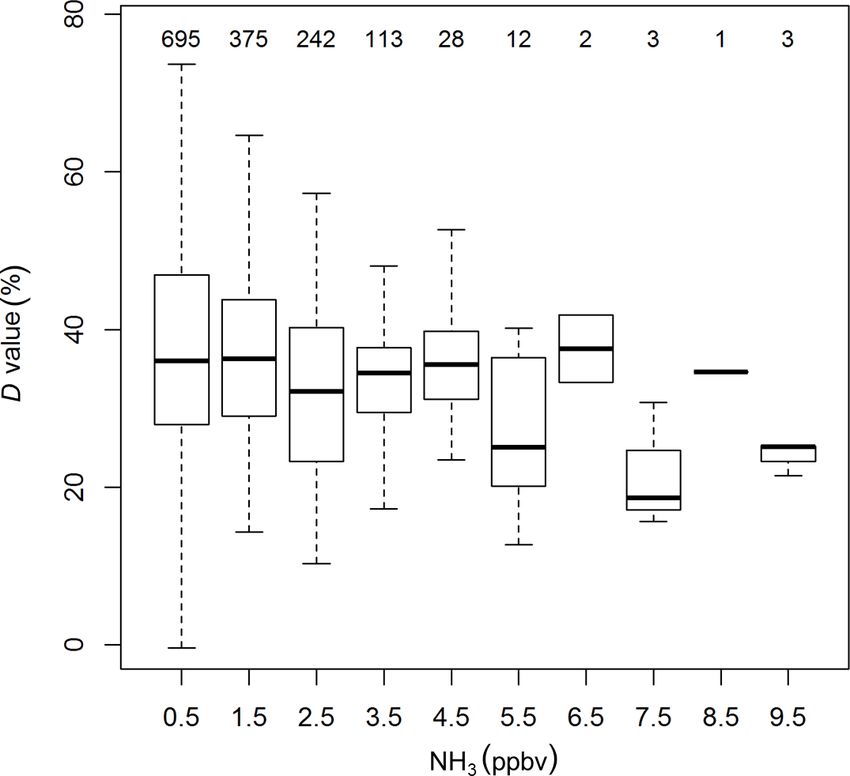
6066                                 A. Moravek et al.: Measurements and quality control of ammonia eddy covariance fluxes

This method accounts for the phase shift and was used in             3     Results
the past to simulate the HFA effect of eddy covariance water
vapour fluxes (Ibrom et al., 2007) and of relaxed eddy accu-
                                                                     3.1    Measured NH3 fluxes, random flux error and flux
mulation systems (Moravek et al., 2013). In the time domain,
                                                                            detection limit (before HFA correction)
a low-pass-filtered scalar time series (catt ) is retrieved as

cattn = cn · A + (1 − A) · cattn ,                            (5)    The QCL eddy covariance measuring system was operated
                                                                     over a period of 149 d between May and October 2017, cov-
where c is the non-attenuated scalar time series and A is the        ering a total of 7132 flux measurement periods. Times of
filter constant. For a given sampling frequency (fs ), this con-     system maintenance, quality control checks and other sys-
stant depends on the cut-off frequency (fc ), which is the fre-      tem downtime were discarded from the dataset, resulting in
quency at which the filter reduces by a power of 2:                  a flux data coverage of around 85 % (Table 1).
                                                                        Figure 3 shows the statistics of flux magnitudes for each
A = 1 − e−2π·(fc /fs ) ,                                      (6)    month from May to October before applying any HFA cor-
                                                                     rection. Flux magnitudes are compared to the median di-
where fc can be characterised by the time constant τ as              urnal flux detection limits of each month. As illustrated in
                                                                     the top-right corner of each month, the diurnal flux mag-
         1                                                           nitudes were comprised of both NH3 emission and deposi-
fc =          .                                               (7)    tion fluxes. Although fluxes in May only represent 4 days,
       2·π ·τ
                                                                     the overall maximum flux of around 500 ng m−2 s−1 was ob-
As the time response for NH3 is described by two time con-           served in that period. While June and July were mainly dom-
stants, we low-pass filtered the high-frequency temperature          inated by small fluxes, typically less than ±10 ng m−2 s−1 ,
time series using both τ1 and τ2 , where τ1 is the time con-         in August clear emission was observed with a daytime me-
stant describing the exchange of sample air volume and τ2            dian value of around 20 ng m−2 s−1 . September marked an
is the time constant accounting for wall interactions. The re-       emission to deposition transition period, with significant de-
spective low-pass-filtered time series, catt1 and catt2 , can then   position fluxes reaching as high as −300 ng m−2 s−1 . In Oc-
be combined as                                                       tober, fluxes were dominated by deposition, with a median
                                                                     daytime value of around −30 ng m−2 s−1 . Over the entire
catt = (1 − D/100) · catt1 + D/100 · catt2 ,                  (8)    period, the daytime median flux was 8.6 ng m−2 s−1 during
                                                                     periods of emission and −19.87 ng m−2 s−1 during periods
using the D value from the time response analysis. The trans-        of deposition (Table 1). Night-time fluxes were significantly
fer function using the time domain low-pass filter method,           lower, with median values of 3.5 and −4.27 ng m−2 s−1 re-
Ttime (f ), is then defined as the ratio between the attenuated      spectively, showing clear diurnal cycles during periods of
and non-attenuation sensible heat flux co-spectrum                   high emission and deposition.
                                                                        The flux statistics are affected by the choice of the flux
               Cowcatt (f )df                                        quality flags used to remove periods of weakly developed
Ttime (f ) =                  .                               (9)
                Cowc (f )df                                          turbulence or non-stationarity (Foken and Wichura, 1996). A
                                                                     quality flag ≤ 3 is typically used for fundamental research,
To account to for the time lag introduced by the phase shift         whereas fluxes with quality flag ≤ 6 are used for long-term
of the low-pass filter, a circular cross-correlation between the     flux datasets. We only used fluxes with a quality flag of ≤ 3,
overall low-pass-filtered temperature and the vertical wind          leaving 68 % of daytime and 46 % of night-time fluxes (Ta-
velocity time series was performed beforehand. The flux at-          ble 1).
tenuation factor using the time response method (αtr ) is then          The random flux error due to instrumental noise (σcov   noise )
determined by the ratio of the filtered co-spectrum and the          is dependent on the precision of the QCL and variations
non-filtered co-spectrum of the sensible heat flux, which is         in the friction velocity (u∗ ). Over the course of the field
equal to the ratio of the attenuated and non-attenuated sensi-       campaign, an average precision of 0.085 (±0.010) ppbv at
ble heat flux covariance:                                            the 10 Hz sample frequency was achieved, which was in-
       R∞                                                            dependent of the measured NH3 mixing ratio. The result-
           CowTatt (f ) df      covhw, catt i                        ing median flux error was 0.17 ng m−2 s−1 for daytime and
αtr = Ro ∞                   =                .             (10)
         o  Co wT (f )df         covhw, ci                           0.08 ng m−2 s−1 for night-time fluxes; much lower than the
                                                                     median observed fluxes (Table 1). In contrast, the random er-
To investigate the possible NH3 flux loss over the measure-                                                 stoch ) was significantly
                                                                     ror derived from the lag time shift (σcov
ment period, the flux loss was simulated for all 30 min pe-          larger, with median values of 1.61 ng m−2 s−1 during day-
riods, using τ1 , τ2 and D values that represent the range of        time and 0.72 ng m−2 s−1 during night-time. However, still
observed time responses.                                             only 11.6 % of the total flux data were below the detection

Atmos. Meas. Tech., 12, 6059–6078, 2019                                                 www.atmos-meas-tech.net/12/6059/2019/
A. Moravek et al.: Measurements and quality control of ammonia eddy covariance fluxes 6067
Table 1. Statistics of the NH3 flux quality control for the flux data collected over the 5-month experiment period. Values given in nanograms
per square metre per second (ng m−2 s−1 ) represent the median value for the period.
Valid flux data Quality control NH3 fluxes Random flux error Flux detection limit (LOD)
QC flag ≤ 3 QC flag ≤ 6 Emission Deposition Instrumental Stochastic LOD = below LOD
(QC flag ≤ 3) (QC flag ≤ 3) noise )
(σcov stoch )
(σcov stoch
2 · σcov (QC flag ≤ 3)
No. % of % of valid % of valid (ng m−2 s−1 ) (ng m−2 s−1 ) (ng m−2 s−1 ) (ng m−2 s−1 ) (ng m−2 s−1 ) (%)
period flux data flux data
Total 6089 85.6 56.8 88.8 6.27 −9.65 0.13 1.08 2.15 11.6
Day 3028 85.0 68.2 93.4 8.59 −19.87 0.17 1.61 3.23 9.4
Night 3061 86.1 45.6 84.3 3.46 −4.27 0.08 0.72 1.43 14.9
Figure 3. Box plot statistics of diurnal absolute NH3 fluxes for each month from May to October 2017 before the application of a HFA
correction. Red lines illustrate the diurnal course of the median flux detection limit. The percentages of flux periods with emission or
deposition are indicated in the top-right corner of each month.
limit (2.15 ng m−2 s−1 ), which shows the overall good per- normalised co-spectra. To illustrate the effect of HFA, the
formance of the QCL eddy covariance measuring system. co-spectra are multiplied by the frequency; HFA is indicated
if the slope of the NH3 co-spectrum in the inertial subrange
3.2 High-frequency attenuation (high frequency part of spectrum) is steeper than the slope of
the sensible heat flux co-spectrum. While this is not clearly
3.2.1 Ogive method visible in the co-spectra (by comparing against the expected
−4/3 slope line in the inertial subrange), the ogives show a
We applied the ogive method to the co-spectra of the sen- clear underestimation of the NH3 flux at higher frequencies,
sible heat and NH3 flux. Figure 4 shows an example of the illustrated by the flattened NH3 ogive curve at high frequen-
www.atmos-meas-tech.net/12/6059/2019/ Atmos. Meas. Tech., 12, 6059–6078, 20196068 A. Moravek et al.: Measurements and quality control of ammonia eddy covariance fluxes
cies. Applying the ogive method to all 30 min periods yields slightly higher than the calculated time constant for the ex-
a frequency distribution of the attenuation factor (Fig. 5). As change of air volume in the 0.5 L absorption cell (∼ 0.1 s).
the ogives may show significant noise or fluctuations, the The time response needed to exchange the air volume in the
choice of the limit frequency for the determination of the inlet tubing is significantly less (< 0.03 s), due to its small
scaling factor is critical. For that reason three limit frequen- volume and low pressure (< 15 kPa) in the inlet tubing. The
cies of 0.050 Hz, 0.067 and 0.100 Hz were chosen represent- time constant τ2 , representing the timescale for NH3 surface
ing timescales of 20, 15 and 10 s respectively. Only periods interactions, showed a median value of 27 s. Both τ1 and τ2
were used where the standard deviation of the scaling fac- did not exhibit a clear trend over time, nor a correlation with
tors determined at those three limit frequencies was smaller humidity or other parameters. In contrast, the D value re-
than 5 %. Furthermore, only data periods were used where vealed distinct differences over time. Figure 7 shows the evo-
both the NH3 and sensible heat flux were significant and of lution of the D value over the course of the field campaign
sufficient data quality (TK3 flag ≤ 3). After applying that fil- as well as times of inlet, tube and cell cleaning. Initially, D
ter, the median flux attenuation factor was calculated to be values were around 20 % and then increased steadily to more
0.83, corresponding to a flux loss of 17 %. The spread of the than 50 % at the end of June. While cleaning of the glass
observed factors was significant with 50 % of the values ly- inlet and the inlet tube in June did not directly lead to a de-
ing between 0.75 and 0.91; the standard deviation was 16 %. crease in the D value, the cleaning of the glass inlet and inlet
Also, for some periods the attenuation factor was above 1, tubing on 27 July led to a visible decrease in the D value.
which was most likely caused by uncertainties in the ogive On 12 September, when the inlet, tubing and the surface of
method. the absorption cell was cleaned, the largest decrease in the D
To give insights into the causes of the NH3 flux loss, the values after cleaning down to 10 % was observed. Addition-
attenuation factor was analysed for dependencies on differ- ally, a significant overall decrease in D values was observed
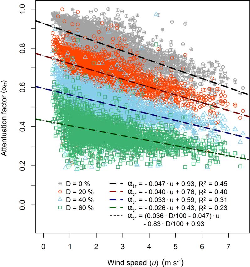
ent parameters. No clear change of attenuation factor was following 17 July , after switching the zero air source from
observed over time, which would have suggested an effect the heating catalyst to the UHP compressed air. As the heat-
of surface ageing or cleaning. Due to the uncertainties in the ing catalyst scrubs NH3 from ambient air, the moisture level
ogive method, the noise in the attenuation factors was larger of the heating catalyst zero air is more similar to ambient
than the effect of surface ageing or cleaning. Also, no corre- air than to that of the dry UHP compressed air. Thus, the D
lation of the attenuation factor with ambient air humidity was value differences for the two zero air sources might be caused
found. The highest variation of attenuation factors occurred by different moisture levels. However, no distinct correlation
at conditions of neutral atmospheric stability, an indication of of the D value with ambient air humidity was found for the
the limitations of the ogive method during these conditions. heating catalyst period. A decrease in D values with increas-
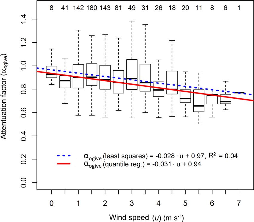
However, a slight decrease in the attenuation factor with in- ing ambient air NH3 mixing ratios, as discussed in Ellis et
creasing horizontal wind speed (u) was found (Figs. 6, S1), al. (2010), was detected (Fig. 8), suggesting a larger relative
which is expected due to the shift of the turbulence spec- importance of adsorption and desorption processes at lower
tra to higher frequencies with increasing wind speed. Given NH3 mixing ratios. The increase in D values at lower NH3
the non-Gaussian distribution of attenuation factors at some mixing ratios may also be due to the variation of D values
wind speeds, we used a quantile linear regression to obtain a caused by a larger uncertainty of the double exponential fit
function of the flux attenuation factor using the ogive method with small mixing ratio changes. While the relative random
(αogive ) with u (in m s−1 ): errors of A1 and A2 from double exponential fit increase ex-
ponentially with decreasing NH3 mixing ratios, the propa-
αogive = f (u) = −0.031 · u + 0.94. (11) gated random error of D was typically below 10 % for NH3
As the majority of data used is clustered between wind mixing ratios above 0.5 ppbv. For lower mixing ratios, only
speeds of 0.5 and 2.5 m s−1 , the correlation with wind speed D values with a relative error of less than 50 % were used.
is only weak as illustrated by a R 2 value of 0.04 of the least
squares linear regression. The correlation might be impacted 3.2.3 Time response method
by changes of the aerodynamic measurement height, due to
tower raise and the growth of the corn canopy over the sea- To investigate the effect of the measured time response on
son. However, as no clear correlation of the attenuation fac- the NH3 fluxes, the flux loss was simulated using the time
tor with time was found, this effect is not accounted for in response method. As the time constants τ1 and τ2 did not
the presented relation with horizontal wind speed. show distinct trends over time like the D value, they were
fixed at 0.6 and 27.0 s respectively. The flux loss was simu-
3.2.2 Time response lated for D values of 0 %, 20 %, 40 % and 60 %, which rep-
resent the observed range of D. Figure 9 shows Ttime (f ) for
The double exponential function used to determine the sys- the four scenarios and their effect on the ogives of sensible
tem’s time response is characterised by τ1 , τ2 and the D heat flux for a selected 30 min period. To illustrate the con-
value. The median value for τ1 was 0.6 s. This value is tributions of the two time constants τ1 and τ2 as well as the
Atmos. Meas. Tech., 12, 6059–6078, 2019 www.atmos-meas-tech.net/12/6059/2019/A. Moravek et al.: Measurements and quality control of ammonia eddy covariance fluxes 6069
Figure 4. Results from the spectral analysis. Panels (a) and (b) show the respective co-spectral densities for the sensible heat and NH3 flux
for the period from 12:00 to 12:30 EST on 9 August 2017. The dashed lines indicate the expected slopes in the low frequency range and the
inertial subrange. (c) The cumulative flux contribution (ogive) for both the sensible heat flux (T ) and the NH3 flux are shown for the same
30 min period. The dashed, dotted and dash-dotted vertical lines represent the limit frequencies used in the flux loss analysis at 0.050, 0.067
and 0.100 Hz respectively.
Figure 5. Results from the ogive analysis show the frequency dis-
tribution of the flux attenuation factor (αogive ). Values lower than
unity represent an underestimation of the NH3 flux. The red verti- Figure 6. Box plot statistics of flux attenuation factors from the
cal line marks the median value of 0.83, corresponding to a flux loss ogive analysis against the binned horizontal wind speed. Numbers
of 17 %. on the top denote the number of data points in each bin. Both the
least square and the quartile regression lines are shown. The coeffi-
cients from the quartile regression were used in Eq. (9).
influence of the phase shift, the respective frequency domain
transfer functions Tf1 (f ) and Tf2 (f ) are shown. As the fre-
quency domain transfer functions used here only account for ulation for flux data from the entire measurement period, a
the attenuation of the signal amplitudes and not the phase clear decrease in the flux attenuation factor with increasing
shift, their sum (Tf (f )) underestimates the flux loss com- horizontal wind speed was observed (Fig. 10), which is ex-
pared with the time domain low-pass filter approach used in plained by a shift of the co-spectrum to higher frequencies
this study. For the 30 min period shown here, the flux loss with increasing wind speeds. The linear regression lines for
ranged from 21 % to 64 %, increasing with higher D values, each simulation scenario are displayed in Fig. 10 including
representing a higher contribution from the slow time con- the respective linear regression functions. By expressing the
stant that reflects adsorption/desorption. Applying the sim- slope (m) and the intercept (c) as a function of D through lin-
www.atmos-meas-tech.net/12/6059/2019/ Atmos. Meas. Tech., 12, 6059–6078, 20196070 A. Moravek et al.: Measurements and quality control of ammonia eddy covariance fluxes
Figure 7. Variation in the time response during the experiment, represented by the D value, as well as times of cleaning of the QCL inlet
system. The D value gives the percentage contribution of time constants associated with wall interactions. Red data points represent the 48 h
moving median D value. To correct for the effect of dry air on the times response, the D values during times when the UHP compressed air
was operated were increased by 20 % (blue data points).
ear regression (fm,c (D) = mm,c · D + cm,c ), we can describe
the flux attenuation factor using the time response method
(αtr ) as a single function of u and the D value as
αtr = f (u, D) = ( mm · D/100 + cm ) · u
+ mc · D/100 + cc . (12)
For the dataset presented, the linear regression yielded mm =
0.036, cm = −0.047, mc = −0.83 and cc = 0.93. The over-
lap of the regression lines of this generalised function with
all individual regression lines in Fig. 10 shows the strong lin-
ear correlation of the flux attenuation factor with both u and
the D value. In the case of D = 0, Eq. (12) represents the
damping that is not due to the wall interactions and would
also be applicable to other, non-sticky, trace gases. After de-
riving αtr , the NH3 fluxes are then corrected individually for
every 30 min period by dividing by αtr .
4 Discussion
Figure 8. Box plots of statistics of time response results: D values
4.1 Random flux error and flux detection limit against the binned ambient NH3 mixing ratios before switching to
the zero air source. Numbers on the top denote the number of data
Closely connected to the issue of HFA is the requirement of points in each bin.
the NH3 measurement system to resolve small NH3 mixing
ratio fluctuations at high time resolution. Due to the chal-
lenges in measuring small NH3 fluxes, the quantification of stoch ). This
cantly lower than the stochastic random error (σcov
the random flux error and flux detection limit is essential for can be attributed to the high precision of the QCL mea-
the quality assessment and interpretation of NH3 fluxes. Dis- surement achieved during the measurement period, resulting
tinguishing between two types of random errors, we found noise of 0.13 ng m−2 s−1 . To our knowledge,
in a median σcov
noise ) was signifi-
that the error due to instrumental noise (σcov continuous wave QCL spectrometers are currently the most
Atmos. Meas. Tech., 12, 6059–6078, 2019 www.atmos-meas-tech.net/12/6059/2019/A. Moravek et al.: Measurements and quality control of ammonia eddy covariance fluxes 6071
Figure 9. Results from the high-frequency loss simulation shown for the period from 12:00 to 12:30 EST on 9 August 2017. (a–d) Calculated
transfer functions for four different scenarios of D (= 0 %, 20 %, 40 % and 60 %) values from the time response fitting procedure. Shown
are the transfer function used in this study, Ttime (f ), where the high-frequency time series was low-pass filtered in the time domain, and
the frequency domain transfer functions, Tf1 (f ) and Tf2 (f ), which illustrate the flux loss associated with τ1 and τ2 respectively. As the
frequency domain transfer functions used here only account for the attenuation of the signal amplitudes and not the phase shift, their sum,
Tf (f ), underestimates the flux loss compared with the time domain low-pass filter approach used in this study. (e–f) The cumulative flux
contribution (ogive) for the non-attenuated and attenuated sensible heat flux and calculated flux attenuation factors (αtr ). For each scenario
the respective transfer function Ttime (f ) in the panel above was used.
precise commercially available NH3 measurement systems. flux detection limit calculation than with our approach. As
As the instrumental noise also affects σcovstoch , σ stoch (median we observed that σcov stoch can vary significantly over time,
cov
1.08 ng m−2 s−1 ) can be used as the total random flux error. when filtering the NH3 flux data the respective flux detection
Investigating the entire measurement period, we found in- limit value of the relevant flux period seems to better reflect
stoch values with a higher (absolute) flux magni-
creasing σcov different turbulence conditions.
tude, although, due to variations, no clear relationship could
be formulated. Still, for (absolute) flux magnitudes above 4.2 Parameters affecting time response
20 ng m−2 s−1 , the median random flux error was 13 %, giv-
ing a general random error estimate for those higher observed The QCL’s time response for NH3 was determined over
flux magnitudes. the 5-month measurement period, providing a large dataset
stoch , the median
Defining the flux detection limit as 2 · σcov of different operational and environmental conditions which
−2 −1
value was 2.15 ng m s , which is about half of what was may impact the time response. Known parameters affecting
reported by Sintermann et al. (2011) for flux measurements the NH3 time response are properties of the ambient air like
using PTR-MS after slurry application (4.5 ng m−2 s−1 ) humidity and magnitude of NH3 mixing ratios, surface ma-
and 4.4 times lower than the detection limit given by terial and surface-adsorbing matter, surface temperature and
Zöll et al. (2016) for measurement above a peatland sample flow conditions. As the temperature of the inlet and
(9.4 ng m−2 s−1 ), utilising the same QCL analyser used in the sample flow rate were not significantly changed during
this study. While our analysis of σcov stoch covered the entire the field campaign, we did not investigate the influence of
measurement period, Sintermann et al. (2011) determined surface temperature and sample flow conditions on time re-
their flux detection limit during a period when no significant sponse. From the findings of our study, in the following we
NH3 fluxes were detected, most likely leading to a smaller discuss and summarise the impact of humidity, ambient NH3
mixing ratios, surface contamination on time response, as
www.atmos-meas-tech.net/12/6059/2019/ Atmos. Meas. Tech., 12, 6059–6078, 2019You can also read