Spatio-temporal analysis of seismic anisotropy associated with the Cook Strait and Kaik oura earthquake sequences in New Zealand
←
→
Page content transcription
If your browser does not render page correctly, please read the page content below
Geophys. J. Int. (2020) 223, 1987–2008                                                                                           doi: 10.1093/gji/ggaa433
Advance Access publication 2020 September 11
GJI Seismology

Spatio-temporal analysis of seismic anisotropy associated with the
Cook Strait and Kaikōura earthquake sequences in New Zealand

Kenny M. Graham ,1 Martha K. Savage ,1 Richard Arnold,2 Hubert J. Zal,1
Tomomi Okada,3 Yoshihisa Iio4 and Satoshi Matsumoto 5
1 Instituteof Geophysics, SGEES, VUW, New Zealand. E-mail: Kenny.Graham@vuw.ac.nz
2 School of Mathematics and Statistics, VUW, New Zealand
3 Graduate School of Science, Tohoku University, Sendai, Japan
4 Disaster Prevention Research Institute, Kyoto University, Uji, Japan
5 Faculty of Sciences, Kyushu University, Shimabara, Japan

                                                                                                                                                            Downloaded from https://academic.oup.com/gji/article/223/3/1987/5904048 by guest on 17 October 2020
Accepted 2020 September 9. Received 2020 April 19; in original form 2020 August 3

                                       SUMMARY
                                       Large earthquakes can diminish and redistribute stress, which can change the stress field
                                       in the Earth’s crust. Seismic anisotropy, measured through shear wave splitting (SWS), is
                                       often considered to be an indicator of stress in the crust because the closure of cracks due
                                       to differential stress leads to waves polarized parallel to the cracks travelling faster than in
                                       the orthogonal direction. We examine spatial and temporal variations in SWS measurements
                                       and the Vp /Vs ratio associated with the 2013 Cook Strait (Seddon, Grassmere) and 2016
                                       Kaikōura earthquakes in New Zealand. These earthquake sequences provide a unique data
                                       set, where clusters of closely spaced earthquakes occurred. We use an automatic, objective
                                       splitting analysis algorithm and automatic local S-phase pickers to expedite the processing
                                       and to minimize observer bias. We present SWS and Vp /Vs measurements for over 40 000
                                       crustal earthquakes across 36 stations spanning close to 5 12 yr between 2013 and 2018. We
                                       obtain a total of 102 260 (out of 398 169) high-quality measurements. We observe significant
                                       spatial variations in the fast polarization orientation, φ. The orientation of gravitational stresses
                                       are consistent with most of the observed anisotropy. However, multiple mechanisms (such as
                                       structural, tectonic stresses and gravitational stresses) may control some of the observed crustal
                                       anisotropy in the study area. Systematic analysis of SWS parameters and Vp /Vs ratios revealed
                                       that apparent temporal variations are caused by variation in earthquake path through spatially
                                       varying media.
                                       Key words: Spatial analysis; Seismic anisotropy; Continental tectonics: strike-slip and trans-
                                       form; Dynamics: gravity and tectonics; Fractures, faults, and high strain deformation zones.

                                                                                method is the inversion of earthquake focal mechanisms to de-
1 I N T RO D U C T I O N
                                                                                termine the stress orientations in the region where the earthquake
Stress in the Earth is an important factor in earthquake genesis.               occurred (Michael 1984; Hardebeck & Michael 2006; Arnold &
Earthquakes are caused by the sudden rupture of rocks along faults              Townend 2007). Geodetic techniques such as using GNSS (Global
exposed to differential stress in the Earth’s crust. Earthquakes oc-            Navigation Satellite System) and InSAR (Interferometric Synthetic
cur when the accumulated shear stress exceeds the strength of faults            Aperture Radar) measurements, which can be used to infer strain
or fractures in rock. Thus, crustal stresses are the immediate driv-            rates, can also be interpreted as changes in stress (Hardebeck &
ing forces of earthquakes (Zoback & Zoback 2002). A variety of                  Michael 2006; Hardebeck & Okada 2018). In most regions, shear
techniques have been devised to measure crustal stress. The most                wave splitting (SWS) parameters can also serve to estimate the
direct technique to determine crustal stress is through strain mea-             orientation of the principal horizontal stresses. Thus, stress orien-
surements in boreholes, where both stress magnitudes and orien-                 tations can be inferred from measuring crustal seismic anisotropy
tations can be determined. However, drilling boreholes to seismo-               through SWS (Crampin 1984; Cochran & Kroll 2015; Savage et al.
genic depths is a difficult and expensive enterprise (Townend &                 2016) and changes in SWS parameters can also be interpreted as
Zoback 2000; Zoback & Zoback 2002). Another well-established                    changes in the state of stress.


C The Author(s) 2020. Published by Oxford University Press on behalf of The Royal Astronomical Society. This is an Open Access

article distributed under the terms of the Creative Commons Attribution License (http://creativecommons.org/licenses/by/4.0/), which
permits unrestricted reuse, distribution, and reproduction in any medium, provided the original work is properly cited.
                                                                                                                                                    1987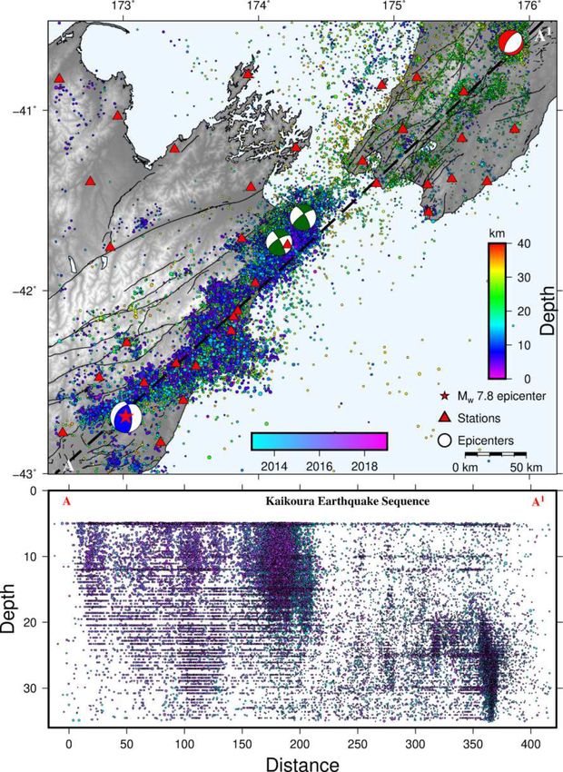
1988       K.M. Graham et al.

   Seismic anisotropy is the dependence of seismic velocity on di-          Dvorkin et al. 1999). Variations in the Vp /Vs ratio have been inter-
rection, as caused by the elastic properties of rocks. The estimation       preted qualitatively by several studies to be related to the movement
of the geometry and strength of seismic anisotropy is often mea-            of fluids in the crust. Li & Vidale (2001) observed an increase in
sured through SWS. SWS is a phenomenon that is observed when                shear velocity of the fault-zone rock around Johnson Valley, af-
shear waves propagating through an anisotropic medium split into            ter the 1992 Mw 7.5 Landers, California, earthquake (from 1994
two nearly perpendicular phases that travel with different velocities.      to 1998). They interpreted the trend as an indication of fault heal-
In the crust anisotropy is often considered to be controlled by either      ing by strengthening after the main shock, which is most likely
stress (stress induced anisotropy) or geological structures (struc-         due to the closure of cracks that opened during the 1992 earth-
turally induced anisotropy) (Crampin 1984; Babuska & Cara 1991;             quake. They also observed that the fault-zone strength recovery
Zinke 2000; Boness & Zoback 2006; Crampin et al. 2015; Savage               is consistent with a decrease in the apparent crack density within
et al. 2016). In the case of stress induced anisotropy, we assume           the fault zone. Moreover, they observed a decrease in the ratio
that cracks or microcracks are randomly distributed. Differential           of traveltime for P to S waves, which they explained as cracks
stress will close cracks perpendicular to the maximum horizontal            near the fault zone being partially fluid-filled and becoming more
stress (SHmax ), leaving open cracks only parallel to SHmax . In the case   fluid saturated with time (Li & Vidale 2001). Chiarabba et al.
of structurally induced anisotropy, the fast wave is oriented paral-        (2009), using S- and P-wave arrival times, observed an increase

                                                                                                                                                      Downloaded from https://academic.oup.com/gji/article/223/3/1987/5904048 by guest on 17 October 2020
lel to structural fabric or the orientation of the residual features of     in Vp /Vs before the Mw 5.3 1997 Umbria-Marche earthquake in
palaeostress (Savage 1999; Cochran et al. 2006). SWS can be char-           central Italy and attributed the trend to a pore pressure increase in
acterized by two parameters, the fast orientation (φ) and the delay         fluid-filled cracks in the volume around the fault. The combination
time (δt). φ is the bearing of the polarization of the faster wave (also    of variations in seismic anisotropy, Vp /Vs ratio and geodetic data
referred to as fast orientations) and δt is the time lag between the        has been reported by recent studies in volcanic areas and a slow-
two split waveforms. δt depends on both the degree of anisotropy            slip region (Savage et al. 2010b; Unglert et al. 2011; Zal et al.
and the path length through the anisotropic medium. Although early          2020).
studies concluded that stress-induced crack alignment is the prin-             Around the Wellington region of New Zealand, Gledhill (1991)
cipal cause of crustal anisotropy (Crampin 1984; Babuska & Cara             and Matcham et al. (2000) used local earthquakes to study the
1991), several later SWS studies, close to and away from the vicin-         anisotropic structure. Audoine et al. (2000) also characterized the
ity of major faults, have concluded that other possible causes of           crustal anisotropy around the transition between the subduction and
crustal anisotropy exist (Matcham et al. 2000; Zinke 2000; Balfour          the oblique transform faulting boundaries. In central MFS, they
et al. 2005; Boness & Zoback 2006). A consistent pattern where φ            observed that fast polarization orientations were subparallel to the
measurements in close proximity to faults show fault-parallel ori-          major faults and geological features, and attributed the observa-
entations and φ measurements further away from faults are parallel          tion to the presence of metamorphosed schist beneath the MFS.
to the principal horizontal stress (orientations) has been reported         At the eastern edges of the MFS, they observed that fast orienta-
around the San Andreas Fault of California, (Zinke 2000; Boness             tions were parallel to the orientation of the maximum horizontal
& Zoback 2006), Wellington region and Marlborough Fault Sys-                compressive stress, SHmax which is consistent with crack-induced
tem (MFS) of New Zealand (Gledhill 1991; Audoine et al. 2000;               anisotropy in the crust. In the North Island, their fast polarization
Matcham et al. 2000; Balfour et al. 2005; Karalliyadda & Savage             orientations were parallel to the strike of the Hikurangi subduc-
2013).                                                                      tion zone as well as to the major geological features (Audoine
   Several researchers have used SWS to measure spatial and tem-            et al. 2000). Balfour et al. (2005) described the upper plate stress
poral variations in seismic anisotropy. Miller & Savage (2001) ob-          regime above the Southern end of the Hikurangi subduction zone,
served changes in fast polarization orientations before and after an        where the dextral MFS accommodates more than 80 per cent of the
eruption at Mt. Ruapehu volcano, New Zealand. They interpreted              relative plate motion (Townend et al. 2012). They examined the
this as a variation in principal stress orientation, which they related     relationship between the SHmax orientations and the average fast ori-
to an increase in stress related to magmatic intrusion or inflation.        entations, and concluded that both stress and structural anisotropy
Roman et al. (2011) observed rotations of fast orientations that            exist around the MFS, but the dominant structural fabric of the
correlated with rotating fault plane solutions for earthquakes asso-        MFS controls the seismic anisotropy measurement rather than SHmax
ciated with volcanic activity at Soufrière Hills volcano in Montser-       (Balfour et al. 2005). Regional stress studies by Townend et al.
rat. Bianco et al. (2006) observed variations in fast orientation and       (2012) and Balfour et al. (2005) around the study area revealed a
delay times before the 2001 eruption on Mt. Etna. They observed             uniform SHmax of 115◦ ± 16◦ , interpreted as the upper plate ex-
delay times exhibiting a sudden decrease shortly before the start           tending across the northern South Island. Recently, Evanzia et al.
of the eruption and variations in the fast orientation five days be-        (2017) tried to distinguish between stresses around Southern Hiku-
fore the onset of the eruption. Zheng et al. (2008) also studied            rangi Margin, New Zealand, using SWS and focal mechanism mea-
the temporal variations of SWS in the aftershock region of 1999             surements. They suggested that stresses in the overriding plate are
Chichi Earthquake, Taiwan. They also observed a decrease in de-             likely related to bending stresses, gravitational stresses and tectonic
lay times shortly before the Chichi main shock and two Chiayi               loading.
earthquakes.                                                                   In this study, we perform a systematic analysis of SWS parameters
   The relation between the ratio of body-wave (P and S waves) ve-          to investigate the physical mechanisms causing crustal anisotropy
locities, Vp /Vs , fluid content and pore pressure are well established     around the Marlborough and Wellington region, and to explore pos-
(e.g. Wadati & Oki 1933; Nur 1971; Ito et al. 1979; Dvorkin et al.          sible temporal variations in SWS measurements. The 2013 Cook
1999, and references therein). The Vp /Vs ratio is one of the best          Strait and 2016 Kaikōura earthquake sequences provide a rare data
parameters to indirectly identify fluid and crack migration within          set, where clusters of closely spaced earthquakes with full azimuthal
the crust, since pore fluid properties produce variations in seis-          coverage occurred. We use this data set to examine the hypotheses of
mic velocities (Dvorkin et al. 1999). In fluid-saturated rocks, high        structure and stress-induced anisotropy that are often used to explain
Vp /Vs anomalies may indicate high pore pressure (e.g. Nur 1971;            anisotropy in the crust. The stress-induced hypothesis suggests that
Spatiotemporal analysis of seismic anisotropy               1989

cracks aligned with the maximum horizontal compressive stress di-                The study area (red box on inset in Fig. 1), central New Zealand,
rection, SHmax , remain open with a preferred orientation (Crampin &          covers the southern end of the Hikurangi subduction zone and the
Booth 1989; Savage 1999) and thus induce anisotropy. The stresses             north eastern part of New Zealand’s South Island, which is domi-
acting on crustal tectonic settings can be characterized into two cat-        nated by the MFS. The MFS marks the transition from a subduction
egories; (i) topographical stresses acting on the shallow crust (often        plate boundary in the north to a transpressive plate boundary (the
referred to as gravitational stresses) and (ii) stresses driven by the        Alpine Fault) in the south. The faults in the MFS are predom-
relative plate motions or geodynamic processes (referred to as tec-           inantly strike-slip (trending NE-SW parallel to the strike of the
tonic stresses). Often, crustal anisotropy studies use SHmax from focal       Pacific-Australia plate motion), with a relatively small component
mechanism inversions to explain the stress hypothesis with little fo-         of reverse motion (Van Dissen & Yeats 1991). The average regional
cus on SHmax from gravitational stresses. Araragi et al. (2015) and           strike of the faults is 55◦ and their near-surface dips vary from 60◦ to
Illsley-Kemp et al. (2017) are two of the few studies that suggested          near-vertical (Van Dissen & Yeats 1991; Anderson et al. 1993). Ma-
gravitational stress as a possible explanation for crustal seismic            jor geological structures around the southern end of the Hikurangi
anisotropy around Mt. Fuji (Japan) and the Northern Afar region               subduction zone strike in the NE-SW direction with active faulting
(East Africa) respectively. In theory, the orientation of gravitation-        also following this NE-SW trend (Mortimer 2004; Litchfield et al.
ally induced horizontal stresses, S HGrav
                                       max
                                           , have different orientations at   2017). Southwest from Kaikōura lies the North Canterbury fold

                                                                                                                                                         Downloaded from https://academic.oup.com/gji/article/223/3/1987/5904048 by guest on 17 October 2020
the peak of a mountain, as opposed to the slopes either side. At the          and thrust belt (Reyners & Cowan 1993; Pettinga et al. 2001). The
peak S HGrav
         max
             is parallel to the strike of the mountain ridge, whereas,        NE-SW trend of the thrust fault extends through the northeastern
on the slope it is perpendicular (Flesch et al. 2001; Hirschberg et al.       part of the Canterbury region. In response to the transition from the
2018). In basins of two mountains ridges, the expected S HGrav  max
                                                                    are of-   subduction related tectonics in the north, thrust faults are evolving
ten perpendicular to the strike of the ridges due to the compressional        (Pettinga et al. 2001). The thrust faults are expressed as topograph-
stresses on the slopes on either side of the basin (Hirschberg et al.         ical ridges with NE-SW strike extending close to the Hope fault
2018). Here, we examine how well both the gravitational and tec-              (Reyners & Cowan 1993; Pettinga et al. 2001). Nearly two-thirds of
tonic stresses explain the crustal anisotropy in central New Zealand          the Marlborough region is underlain by greywacke of the Torlesse
(southern North Island and northwestern south island; see Fig. 1) by          Supergroup, a laterally uniform wave-speed structure (Reyners &
comparing the splitting measurements with SHmax from both gravita-            Cowan 1993; Mortimer 2004). The Marlborough Schist found north
tional and tectonic stresses (stresses at depth from focal mechanism          of the Wairau fault, which is part of the Haast Schist of South Island,
inversion).                                                                   is commonly considered to be strongly metamorphosed (Mortimer
   The structurally controlled hypothesis suggests that the orien-            1993).
tation of the anisotropic medium is associated with the orienta-                 The 2013 Cook Strait earthquake sequence started in 2013 July
tion of the geological structures (such as fault orientations, shear          with two foreshocks of Mw 5.7 and 5.8 and climaxed in the 2013
planes subparallel to faults) (Zinke 2000; Boness & Zoback 2006;              July 21, Mw 6.5 Seddon earthquake and the 2013 August 16,
Cochran et al. 2006; Okaya et al. 2016). Mineral alignment, asso-             Mw 6.6 Lake Grassmere earthquake (Fig. 1). These large earth-
ciated with shearing in fault zones, or foliation in metamorphosed            quakes, located ∼50 km south of Wellington, New Zealand’s capital,
rocks has been one of the hypotheses used to explain structurally             generated significant ground shaking in the Wellington and Marl-
controlled anisotropy in the crust. Around central New Zealand,               borough regions (Holden et al. 2013; Hamling et al. 2014). Both
Audoine et al. (2000) attributed the observed anisotropy to the               earthquakes were strike-slip events with similar magnitudes and
metamorphosed schist in the crust because recrystallization dur-              characteristics and they were considered to be a ‘doublet’ (Holden
ing metamorphism may form schistosity or a pervasive foliation.               et al. 2013). The seismicity in the Cook Strait sequence region is
Okaya et al. (1995) also observed a high degree (up to 20 per cent)           still above the background levels that existed prior to 2013, with
of anisotropy associated with the Haast Schist of the South Island,           more than 16 000 earthquakes (ML ≥ 1) within a 4 yr period from
New Zealand. Okaya et al. (2016) explained the crustal anisotropy             2013 January to 2017 November (Holden et al. 2013; GeoNet 2019,
in the Taiwan collision zone by deformation-related (due to perva-            accessed 2019 February 2). Seismicity in Marlborough (before the
sive shearing in strike-slip fault zones) mineral preferred orienta-          2016 Kaikōura earthquake) was mainly concentrated in the region
tion in the metamorphic rocks (e.g. schist fabric). In this paper, we         above the subduction interface and around the north-eastern part
examine these various hypotheses by comparing our splitting mea-              of the MFS (Holden et al. 2013). The area was the location of a
surements with active fault orientations, orientations of horizon-            swarm of M > 4 earthquakes in 2005 and before that, it was the
tal principal stress (both tectonic and gravitational) and maximum            location of the 1977 M 6 Cape Campbell earthquake and the 1966
shear plane orientations from the strain rate field (related to crustal       M 5.8 Seddon earthquake (Holden et al. 2013). Six months after the
deformation).                                                                 Mw 6.6 Lake Grassmere earthquake, the 2014 Mw 6.2 Eketahuna
                                                                              earthquake struck 10 km east of Eketahuna. The depth (34 km) and
                                                                              location of the event placed it below the interface between the sub-
                                                                              ducting Pacific plate and overriding Australian plate (Abercrombie
2 TECTONIC SETTING AND
                                                                              et al. 2016). The afterhocks of the 2014 Eketahuna earthquake are
SEISMICITY
                                                                              characterized by repeating events (Wallace et al. 2017).
New Zealand’s tectonic setting is characterized by two subduction                The Mw 7.8, 2016 November 14, Kaikōura earthquake, is the
systems of opposite polarity, connected by an area of oblique con-            largest and most complex earthquake recorded on land in New
tinental convergence (inset in Fig. 1). Westward subduction (and              Zealand (Clark et al. 2017; Hamling et al. 2017). The earthquake
intra-arc rifting) in the North Island at the Hikurangi subduction            initiated near the North Canterbury region at a depth of 15 km with
zone changes to strike-slip at the Marlborough Fault Zone, trans-             an oblique thrust faulting mechanism (Hamling et al. 2017, fig. 1).
pressional collision along the Alpine Fault and finally back to (east-        The rupture propagated from south-west towards the north-east for
ward) subduction at the Puysegur Trench (inset in Fig. 1) offshore            about 120 s, with an unusual source process, starting with weak
(Mortimer 2004).                                                              radiation and releasing more energy while propagating towards the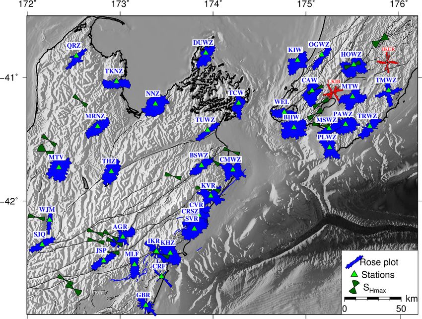
1990       K.M. Graham et al.

                                                                                                                                                                   Downloaded from https://academic.oup.com/gji/article/223/3/1987/5904048 by guest on 17 October 2020
Figure 1. Map showing the tectonic setting of the study area with the stations used (red and blue triangles) plotted on a basemap of the digital topography and
bathymetry (Mitchell et al. 2012). GeoNet CMT solutions of Mw > 6 earthquakes from 2013 to 2018 are shown; blue focal mechanism plots (beach balls)
represent reverse mechanisms, with the red representing normal faulting with some dip slip motion and green represents a strike-slip mechanism. Major faults
marked include the Wairau (WF), Awatere (AF), Clarence (CF) and Hope (HF) faults. The red lines denote the surface rupture of faults during Kaikōura main
shock (Langridge et al. 2016). The yellow star indicates the epicenter of the Mw 7.8 Kaikōura earthquake. Inset: the study region (red frame): the blue line is
the plate boundary fault showing the Hikurangi and Puysegur trenches.

north-east over a distance of ∼150 km and terminating offshore in                  3 D ATA A N D M E T H O D O L O G Y
the Cook Strait region (Cesca et al. 2017; Duputel & Rivera 2017;
Holden et al. 2017; Hamling et al. 2017). A remarkable number                      3.1 Data
(>20) of shallow crustal fault segments (involving a combination
                                                                                   We determine SWS measurements for over 40 000 local crustal
of reverse and dextral strike-slip faulting; Fig. 1) ruptured, including
                                                                                   earthquakes that were located around the region of the 2013 Cook
vertical motions of more than 10 m and horizontal displacements
                                                                                   Strait earthquake sequence (Fig. 2). Our earthquake catalogue con-
over 11 m (Clark et al. 2017; Cesca et al. 2017; Hamling et al.
                                                                                   sists of GeoNet detection and locations (Petersen et al. 2011) and
2017). Most of the faults that ruptured have a general NE-SW trend
                                                                                   spans more than 5 yr: from 2013 January to 2018 June. Although
(red lines in Fig. 1), but some have NW-SE orientation, revealing a
                                                                                   Lanza et al. (2019) relocated some of the events used here, we used
complex and heterogeneous slip pattern (Clark et al. 2017; Hamling
                                                                                   the GeoNet catalogue to ensure consistency. The GeoNet catalogue
et al. 2017; Kaiser et al. 2017). Surface rupture was mostly asso-
                                                                                   used here has a good azimuthal coverage of events before and after
ciated with known onshore faults. However, some surface traces
                                                                                   the 2016 Kaikōura main shock (see Fig. S1, Supporting Informa-
were produced by faults that had not been previously mapped. Also
                                                                                   tion). This enables us to search for temporal variations in SWS
some faults ruptured offshore, causing a small tsunami (Clark et al.
                                                                                   parameters and Vp /Vs ratios.
2017; Wallace et al. 2017). The 2016 Kaikōura earthquake was fol-
                                                                                      We use 36 stations deployed around the Wellington and Marl-
lowed by more than 25,000 local and regional aftershocks (GeoNet
                                                                                   borough region. These stations include 24 permanent seismic sta-
catalogue), clustered in three unique spatial patterns (Kaiser et al.
                                                                                   tions (combination of broad-band and short-period instruments;
2017). More than 100 000 landslides were triggered by the earth-
                                                                                   red triangles on Fig. 1) operated by GeoNet (the Geological haz-
quake and subsequent aftershocks, with 50 of them yielding signif-
                                                                                   ard information for New Zealand) and 12 temporary short-period
icant landslide dams (Litchfield et al. 2017; Dellow et al. 2017).
                                                                                   stations installed and operated by DPRI (Disaster Prevention Re-
Another unusual aspect of the Kaikōura earthquake was the occur-
                                                                                   search Institute, Kyoto University, Japan) (Okada et al. 2019)
rence of large-scale (>15 000 km2 ) slow-slip events triggered on
                                                                                   at different time periods between 2009 and 2018 (blue triangles
the central and northern Hikurangi subduction interface (250 and
                                                                                   on Fig. 1). Plots of data continuity for all stations are shown
600 km away from the epicentre, respectively) due to dynamic-stress
                                                                                   in Supporting Information S2. All the stations were re-sampled
changes from passing seismic waves (Wallace et al. 2017).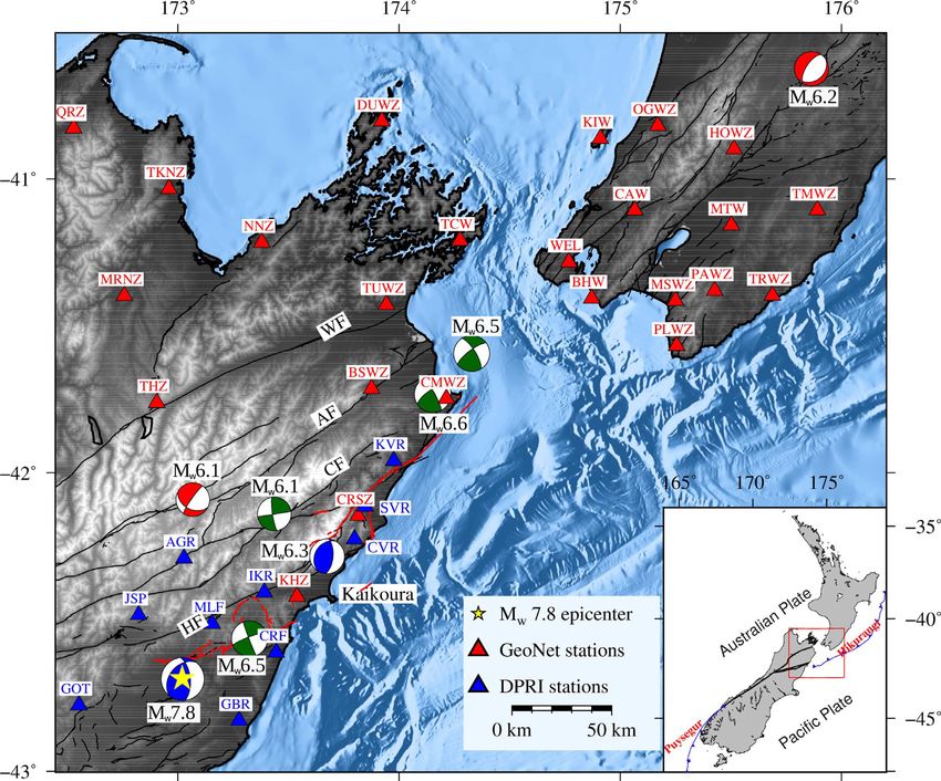
Spatiotemporal analysis of seismic anisotropy 1991
Downloaded from https://academic.oup.com/gji/article/223/3/1987/5904048 by guest on 17 October 2020
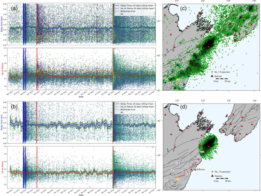
Figure 2. Map of earthquake epicentres used for analysis. Red triangles are the locations of GeoNet stations used. Events are colour-coded by the hypocentral
depths. Blue focal mechanism solution (beach ball) represents the Kaikōura earthquake faulting mechanism; red beach ball represents the Eketahuna earthquake
faulting mechanism, and green beach balls represent the two Cook Strait sequence earthquake faulting mechanisms (Ristau 2013). Focal mechanisms solutions
were obtained from the GeoNet regional moment tensor solution catalog. A cross-section from A to A1 shows the projected depth distributions, coloured by
time (timescale on main figure).
with a common sampling frequency of 100 Hz. Since the objec- 3.2 Method
tive was to study crustal anisotropy, the hypocentral depths were
To estimate SWS parameters for thousands of waveforms, a fully
limited to less than 35 km to include only earthquakes whose
automated and systematic technique was implemented. Here, we
ray paths travel wholly through the crust. Moreover, we limited
used the automatic splitting analysis code. Multiple Filter Auto-
events magnitudes to Mw 1.5 and above to remove any poor-quality
matic Splitting Technique (MFAST, Savage et al. 2010a; Wes-
waveforms.
sel 2010), which is designed to handle large volumes of data.
1992       K.M. Graham et al.

MFAST is based on the eigenvalue-minimization method of Sil-                 component seismogram to estimate the S-phase arrival. See Diehl
ver & Chan (1991) and the clustering method of Teanby et al.                 et al. (2009) and Castellazzi et al. (2015) for further details on the
(2004a). MFAST uses an automated workflow to estimate the                    algorithm.
splitting parameters with an objective grading of measurements                  We calibrated the picking algorithm with over 3500 manually
(Walsh et al. 2013). A concise description for MFAST is pre-                 picked S phases. These S phases were randomly selected to obtain
sented in Section 3.2.2 and a detailed description of the method             a uniform station, magnitude and depth distribution. The time dif-
is presented by Savage et al. (2010a), Wessel (2010) and Walsh               ference between manual and Spicker picks revealed a symmetrical
(2012).                                                                      unimodal distribution with a mean of 0.030 s and a standard devia-
    We used P-wave arrival times and origin times, to determined             tion of 0.598 s. In addition, 90 per cent percent of the Spicker picks
by GeoNet (Petersen et al. 2011). We used an automatic algorithm             were within ±0.484 s of the manual S picks (Fig. 3a). This picking
(Section 3.2.1) to estimate local shear wave arrival times for seismo-       accuracy is adequate for our studies, because MFAST uses multiple
graphs with good signal-to-noise ratio (SNR > 3). All SWS mea-               windows for its analyses. The best parameters (Table S1, Support-
surements were made within the ‘shear wave window’ (incidence                ing Information) that yielded more picks and small time difference
angles less than a chosen critical angle, defined below). We used 1-D        between manual and Spicker picks were used for the final pick-
synthetic analysis (determining the effect of angle of incidence on          ing. We compared the common S picks (∼21 000) between GeoNet

                                                                                                                                                      Downloaded from https://academic.oup.com/gji/article/223/3/1987/5904048 by guest on 17 October 2020
splitting measurements) to resolve the ultimate critical angle for our       manual S and Spicker picks across all stations. The time difference
analysis. This was necessary because, outside the shear wave win-            between GeoNet manual S and Spicker picks revealed a symmetric
dow, the shear waveforms are susceptible to S to P conversions and           unimodal distribution with mean 0.028, standard deviation 0.648
scattering at the surface causing nonlinear particle motion (Nut-            and 90 per cent of the picks were within ±0.678 (Fig. 3b). Over
tli 1961; Crampin & Gao 2006; Savage et al. 2016). Neuberg &                 200 000 S phases were obtained, representing about 23 per cent of
Pointer (2000) showed that waveforms outside the shear wave win-             the expected (event-station pair) arrivals. To assess the quality of
dow generate elliptical particle motion even without the presence            the S picks across our data set, we randomly selected approximately
of anisotropy, especially when recording shallow local earthquakes           5 per cent of the S picks across all stations. The selected events
in the vicinity of strong topography. We simulated waveforms in a            were manually inspected and approximately 15 per cent of S picks
1-D anisotropic medium using the Levin & Park (1997) 1-D reflec-             were unreliable and were either revised or discarded. Based on this
tivity code (which was subsequently modified by Castellazzi et al.           analysis we estimate approximately 85 per cent of the S picks are
2015; Walsh 2012) and estimated the apparent splitting parameters            reliable.
using MFAST (Wessel 2010; Savage et al. 2010a). Fig. S3 in the                  Some of components of the short-period stations operated by
Supporting Information shows the 1-D model used for analysis.                DPRI were intermittently missing components. We could not apply
The effect of angle of incidence on splitting analysis was tested by         the Spicker technique to estimate the S-phase arrival, since the
varying angle of incidence with backazimuth. As shown in Fig. S4             technique required all three components for the estimation. Instead
in the Supporting Information, we observed a strong backazimuthal            we used the Generalized Seismic Phase Detection (GPD), technique
variation of δt and φ as angle of incidence is increased (here vertical      developed by Ross et al. (2018) for estimating phase arrivals for
incidence is 0◦ ). At higher angle of incidence > 30◦ , we observe sig-      the DPRI stations. This technique trained a convolutional neural
nificant variations of splitting parameters with backazimuth. Since          network (a deep learning framework) to learn the features of seismic
we observed less variations of splitting parameters with backaz-             waveforms. An already trained model can be applied to waveforms
imuth at an incidence angle of 35◦ compared to higher incidence              that are not included in the training set, thus a trained model can
angle, we selected a maximum angle of 35◦ as the best shear wave             be applied to different tectonic settings (Kong et al. 2018; Ross
window for our analysis. We estimated angles of incidence using              et al. 2018). We used the Ross et al. (2018) GPD-framework model
the TauP toolkit (Crotwell et al. 1999) and a 1-D velocity model             which they trained and validated with a total of 4.5 million three-
extracted from the Eberhart-Phillips & Fry (2018) 3-D velocity               component waveforms across a range of magnitudes. With each
model.                                                                       component’s time-series, the model predicts the probability that
                                                                             a phase arrival is either a P or S arrival. We set the minimum
                                                                             probability for phase detection to 95 per cent. An example of a pick
                                                                             example is shown in Fig. S5 in the Supporting Information. To gain
3.2.1 Local phase arrival picking
                                                                             confidence in the GDP picks, we estimated P- and S-arrival times
Determination of S-wave arrival times is necessary to estimate SWS           for events with GeoNet manual S picks (more than 40 000 picks
measurements. Due to the large volume of our data set, manually              across the 24 permanent GeoNet stations) and compared the time
picking the S-phase arrival times would have been too time con-              difference between the GDP and GeoNet manual S picks. The time
suming. We therefore used two automatic picking techniques. First,           difference shows a concentrated symmetric uni-modal distribution
local S-phase arrival times (S picks) for GeoNet stations were auto-         with mean −0.072 s, standard deviation 0.774 s and 90 per cent
matically picked using the technique of Diehl et al. (2009) modified         percent of the picks were within ±0.261 s (see Fig. S6, Supporting
by Castellazzi et al. (2015), hereafter called Spicker. For stable and       Information).
reliable S-wave picking, the Spicker technique combines three dif-
ferent detection and picking methods. The STA/LTA (Short Term
Averaging / Long Term Averaging) detector (e.g. Allen 1978) and              3.2.2 Measuring splitting parameters
polarization detector (e.g. Flinn 1965) are used to identify the first       SWS parameters were estimated using the MFAST code (Savage
arriving S phase. The information provided by the detectors is then          et al. 2010a; Wessel 2010). This procedure finds the inverse
used to set up the search windows of the autoregressive picker               splitting operator that best removes the splitting. The waveforms
using the Akaike Information Criterion (AR-AIC) as outlined by               are filtered with a series of bandpass filters, and the product of
Takanami & Kitagawa (1988). Finally, all three methods are com-              the bandwidth and the SNR of the filtered waveform is used
bined to yield the best arrival time of the first arriving S phase and its   to determine the best three filters. Splitting measurements for
corresponding uncertainty. The Spicker makes use of all the three            all three filtered waveforms are estimated using the Silver &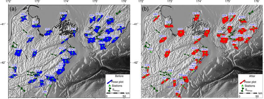
Spatiotemporal analysis of seismic anisotropy                  1993

Figure 3. Distributions of local S-phase picking errors relative to analyst pick. (a) Time difference between Spicker picks and manually picked S-phase arrival
times. (b) Time difference between GeoNet manual and Spicker picks.

                                                                                                                                                                  Downloaded from https://academic.oup.com/gji/article/223/3/1987/5904048 by guest on 17 October 2020
Chan (1991) and Teanby et al. (2004b) method with modifica-                           We also estimated the percent anisotropy, κ, following the ap-
tion by Walsh et al. (2013). The splitting parameters are estimated                proach of Babuska & Cara (1991) and Savage (1999). Here, we
using the eigenvalue minimization method repeated over multiple                    define κ = (vmax − vmin )/v̄. Where vmax is velocity of the shear
time windows around the S phase. The splitting parameter pair                      wave along the fast orientation, vmin is the velocity of the shear
(φ, δt) that best removes the splitting as measured by the small-                  wave along the slow orientation and v̄ is an average of vmax
est eigenvalue of the corrected covariance matrix, is chosen as                    and vmin . Assuming both fast and slow waves travel with the
the best measurement for the given time window (Savage et al.                      same path length, κ can be related to δt as: κ = 200∗δt/(2ts
2010a).                                                                            + δt). We use κ as well as δt, to characterize the anisotropy
    This procedure is then repeated for 75 windows covering                        structure.
slightly different time spans around the S phase. The windows are
automatically selected based on the dominant period around the
filtered shear wave (Savage et al. 2010a). Cluster analysis over
                                                                                   3.2.3 Spatial averaging
the 75 window measurements is used to select the final splitting
parameter for the filter under consideration and to calculate the un-              SWS measurements provide an estimate of the anisotropy along the
certainty associated with the measurements (Teanby et al. 2004a).                  ray propagation path between the source and station. However, it can
Measurements are graded from A to D depending on the consis-                       be difficult to determine exactly where along the ray propagation
tency between the (φ, δt) and measurements in the different win-                   path the anisotropy originates. With measurements from several
dows. MFAST also provides a measure of the incoming polariza-                      stations and a dense cluster of events, one can probe the spatial
tion orientation (φ in ) by estimating the eigenvalues of the corrected            variation of φ and δt using a spatial averaging technique. We used
components after splitting is removed (Silver & Chan 1991; Sav-                    the TESSA (Tomography Estimate and Shear wave splitting Spatial
age et al. 2010a). φ in corresponds to the polarization orientation                Average) technique by Johnson et al. (2011) to estimate the spatial
of the shear wave before it enters the anisotropic layer responsi-                 averages of φ.
ble for the measured splitting parameters. As a quality control,                      For the spatial averaging technique, the study area is divided into
we removed all null graded measurements (events for which no                       cells or blocks using the recursive quadtree clustering algorithm
measurable splitting occurs or event for which φ is within 20◦ of                  described by Townend & Zoback (2001). We set the minimum block
parallel or perpendicular to φ in ) and also kept only A and B graded              size to 5 km2 and the minimum and maximum number of ray paths
measurements. We also limited maximum delay times, δt to 0.4 s                     to be 20 and 80, respectively. The quadtree gridding algorithm works
since local crustal events are often not expected to have larger de-               in an iterative process. Cells with less than 20 rays passing through
lay times (Balfour et al. 2005; Cochran & Kroll 2015). Following                   are not used for analysis and those with more than 80 rays passing
the quality control, a total of 102 260 (out of 398 169) high-quality              through are subdivided until a minimum of block size of 5 km2 or
measurements were obtained. Wessel (2010), Savage et al. (2010a)                   until a minimum number of 20 events is attained. These criteria
and Walsh et al. (2013) give a detailed description of the MFAST                   were chosen to ensure that each block contained enough data to
method.                                                                            give a reliable average measurement. To take into account variations
    We estimated Vp /Vs ratios along the ray path of each event                    due to heterogeneous anisotropic structure along the ray path (e.g.
that yielded high quality SWS measurements to each station us-                     Rümpker & Silver 1998; Johnson et al. 2011), rays in each grid cell
ing the approach of Wadati & Oki (1933) and Nur (1971). We                         are weighted by the inverse of the distance squared (1/d2 ) (where
assumed a linear ray path and that the Vp /Vs ratio is homo-                       d is the distance from the station to the grid cell in question). This
geneous along the seismic wave’s path (Kisslinger & Engdahl                        weighting scheme is used because we expect splitting to occur later
1973). The Vp /Vs ratio of each event-station pair was calculated                  in the ray path and we did not observe a strong correlation between
using Vp /Vs = (ts − to )/(tp − to ), where ts and tp are the ar-                  δt and hypocentral depth (Johnson et al. 2011). For comparisons
rival times of the S and P waves, respectively and to is the event                 with time, we used the regular gridding to ensure that the data
origin time (from the GeoNet catalogue). Only Vp /Vs values be-                    points are always at the same locations. The spatial averages of φ
tween 1.5 and 2.3 were used because values outside of this range                   are computed using a circular statistics approach (Berens 2009) and
are not expected around the study region (Eberhart-Phillips &                      are estimated only when the standard deviation of fast orientations
Fry 2018) and would probably be due to inaccurate arrival time                     in each grid is less than 30◦ and the standard error of the mean is less
picks.                                                                             than 10◦ .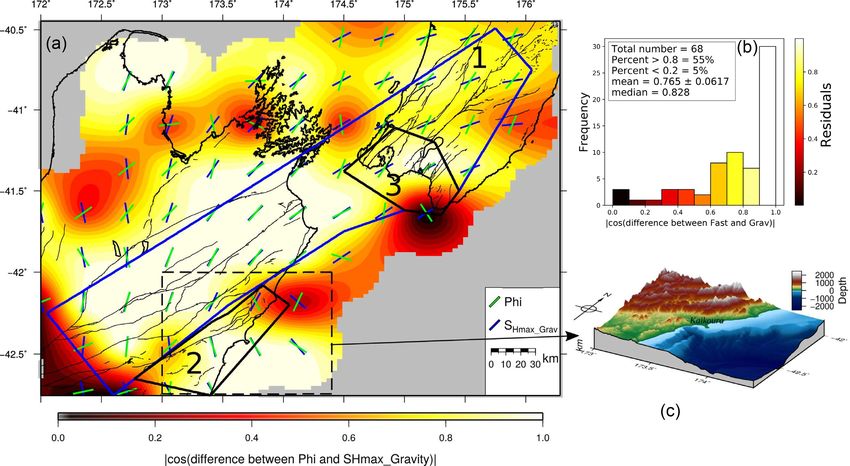
1994      K.M. Graham et al.

3.2.4 Quantitative comparison of φ measurements                         eastern coastal edge of the MFS yield NW-SE orientations of φ,
                                                                        which is perpendicular to the structural trend and subparallel to the
We made quantitative comparisons of our spatially averaged φ mea-
                                                                        crustal SHmax orientations. At station CMWZ and KVR, we observe
surement with GNSS derived principal contraction axes, average
                                                                        a bi-modal distribution of φ orientations, with one subset subpar-
fault orientations, gravitational stress and focal mechanism inver-
                                                                        allel to the SHmax orientation and the other subset subparallel to
sion measurements. We also quantitatively compared averaged φ
                                                                        the strike of the faults. At stations BSWZ and TUWZ, φ orienta-
measurements between events before and after the 2016 Kaikōura
                                                                        tions are subparallel to the orientation of the nearby Awatere and
earthquake to observe any spatiotemporal variation associated with
                                                                        Wairau Faults respectively and perpendicular to the nearby SHmax
the 2016 Kaikōura main shock. For our quantitative comparison,
                                                                        orientation.
we estimate a test statistic, F, the absolute value of the cosine of
                                                                           Around the southern end of the North island, the φ orientation at
the difference between the two angles (F = |cos (ψ 1 − ψ 2 )|) where
                                                                        most stations exhibit significant variations from each other. Some
ψ 1 is the mean φ measurement and ψ 2 is the comparison angle.
                                                                        stations exhibit a bi-modal distribution while others show a domi-
Since we do not have an identical set of locations at which mean φ
                                                                        nant NE-SW direction, with a few stations exhibiting trends that are
has been estimated, we use locations that are closest together, and
                                                                        neither parallel to SHmax nor to the strike the major faults. At stations
< 10 km to estimate the residual. Values of F range from 0 to 1,
                                                                        TMWZ and MTW, a clear bi-modal distribution of fast polarization
where 1 represents parallel orientation and 0 represents perpendic-

                                                                                                                                                    Downloaded from https://academic.oup.com/gji/article/223/3/1987/5904048 by guest on 17 October 2020
                                                                        orientation is observed. One subset trends NE-SW and the other
ular orientation between ψ 1 and ψ 2 . We contour the residual using
                                                                        subset trends NW-SE (Fig. 4).
the GMT functions grdsample and grdimage (Wessel et al. 2013).
                                                                           To investigate temporal variations resulting from the 2016
We also estimate the mean and median of the F to give an indication
                                                                        Kaikōura main shock, φ measurements were split into two sub-
of how well the two angles are correlated.
                                                                        sets: before (from 2013 January 01 to 2016 November 16) and
                                                                        after (from 2016 November 14 to 2018 June 30) the Kaikōura main
3.2.5 Averaging for time variations                                     shock. The 2013 Cook Strait earthquake sequence produced ample
                                                                        seismicity to determine the background φ orientation prior to the
To examine variations we employed an averaging technique for            2016 Kaikōura main shock. Fig. 5 shows rose diagrams of φ mea-
values of δt to smooth and minimize the scatter as much as pos-         surements before (Fig. 5a) and after the 2016 Kaikōura main shock
sible. We use a simple moving median as the smoothing func-             (Fig. 5b).
tion that reduces the noise in the measurement. We used a 20-d
moving median filter on the individual results with the aim of re-
moving the scattered values from the data set. We estimate the
95 per cent confidence intervals by using the non-parametric boot-      4.1 Spatial averaging
strap approach. In this approach, we randomly sample with re-           Using the technique described in Section 3.2.3, we performed spa-
placement from the original sample a data set of the same size as       tial averaging analysis for more than 102 260 source–receiver φ
the original sample. We repeat this for 1000 replicates and for each    measurements. Based on the criteria outlined in Section 3.2.3,
replicate data set we estimate the median value. The 2.5th and 97.5th   4579 out of 4720 grid elements created were used for analysis
percentile of the replicate data set is estimated as the respective     (see Fig. S7, Supporting Information). Circular averages of φ mea-
lower and upper values of the 95 per cent confidence interval for the   surements in each grid square are represented by bar (coloured
median.                                                                 by mean φ value) and plotted at the centre of each grid square
                                                                        (Fig. 6). The spatial averaging results shows a significant spa-
                                                                        tial variation. We observe a dominant NE-SW (see yellow bars
4 R E S U LT S
                                                                        on Fig. 6) trend, which is subparallel to the strike of the ma-
We determined SWS measurements for more than 40 000 wave-               jor active faults and also the topographic trends. We also note
forms recorded on at least one of the 36 stations within the study      a clear contrast of perpendicular fast orientations (blue bars on
region (Fig. 1). Tables 1 and 2 give a summary of fast orientations,    Fig. 6) around the eastern end of the MFS (the region that rup-
delay times, percentage of anisotropy and Vp /Vs ratio as well as       tured during the Kaikōura earthquake). This NW-SE feature ex-
associated descriptive statistics for each station. Out of ∼102 000     isted before the 2016 Kaikōura sequence (see Fig. S8, Supporting
high-quality SWS parameters we estimated, the delay times vary          Information).
between near zero to 0.372 s with an average of 0.157±0.001 s. The         To investigate the spatiotemporal variation of φ measurements
Vp /Vs ratio varies from 1.58 to 2.22 with an average of 1.741±0.001.   associated with the 2016 Kaikōura main shock we performed spa-
Percent anisotropy varies from 0 to 5.186 per cent with an average      tial averaging analysis for events before and after the earthquake.
of 0.922±0.004 per cent.                                                Using the method described in Section 3.2.4, we made quantitative
   Rose diagrams of φ orientations recorded at each station, overlain   comparisons of our spatially averaged φ measurements between
on a basemap of the digital topography, are shown on Fig. 4. SHmax      events before and after the 2016 Kaikōura main shock to search
orientations from Townend et al. (2012) and Balfour et al. (2005) are   for potential spatiotemporal variations associated with the 2016
also shown as green bow ties with wedges showing the 95 per cent        Kaikōura main shock. The orientations of spatially averaged re-
confidence interval. φ orientations for most of the stations show       sults for before (green bars) and after (blue bars) are shown in
a dominant NE-SW orientation, which is parallel to the strike of        Fig. 7. Generally, the orientations of the two angles are in agree-
the geological structures in the region. A few stations have NW-SE      ment, which indicates no significant spatiotemporal variation (in
orientations.                                                           most cases the blue after bar is invisible under the exactly matching
   Around the MFS, φ orientations are generally parallel to the         green before bar). The mean and median value of F (Section 3.2.4)
strike of the active faults. The consistent trend suggests a relation   is 0.92 ± 0.011 and 0.99 respectively (thus a mean and median
between φ and the structural trend around the central and west-         difference of 23◦ and 10◦ respectively) indicates a strong agreement
ern MFS. Yet, some stations, KHZ, IKR, CRF and GBR, at the              between the orientations before and after the main shock. Out of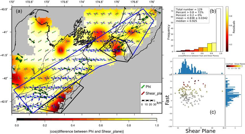
Spatiotemporal analysis of seismic anisotropy                  1995

Table 1. Summary statistics of fast orientation (φ), delay time (δt), Vp /Vs ratio and percent anisotropy (per cent Aniso) with their 95 per cent confidence
interval for GeoNet permanent stations
                                                                                                                                                Per cent Aniso
Station      Events        Mean φ(◦ )        SD φ         Mean δt(s)        SD δt        Mean Vp /Vs         SD Vp /Vs    Mean per cent Aniso         SD
BHW           3515       81.14 ± 7.40        62.82       0.136±0.002        0.066       1.724±0.002            0.066         0.759±0.015            0.424
BSWZ          4781       52.82 ± 1.76        43.38       0.181±0.002        0.076       1.743±0.002            0.084         1.453±0.023            0.801
CAW           6499       17.05 ± 3.29        55.91       0.171±0.002        0.081       1.744±0.001            0.051         0.683±0.009            0.342
CMWZ          2162       -82.10 ± 10.43      64.11       0.173±0.003        0.072       1.819±0.008            0.181         2.371±0.065            1.534
CRSZ          1588       67.47 ± 4.07        48.34       0.168±0.004        0.085       1.808±0.014            0.281         2.118±0.060            1.167
DUWZ          2639       28.60 ± 3.68        50.79       0.203±0.003        0.086       1.738±0.002            0.044         0.623±0.011            0.262
HOWZ          2015       69.93 ± 6.58        57.45       0.139±0.003        0.075       1.732±0.002            0.045         0.673±0.019            0.419
KHZ           6343       -32.95 ± 2.89       53.83       0.149±0.002        0.073       1.736±0.001            0.055         0.713±0.011            0.421
KIW           5497       53.85 ± 3.11        53.87       0.152±0.002        0.073       1.718±0.001            0.044         0.629±0.008            0.296
MRNZ          2375       52.98 ± 3.78        50.37       0.205±0.003        0.081       1.741±0.001            0.030         0.535±0.009            0.214
MSWZ          3481       60.46 ± 2.02        43.02       0.142±0.003        0.077       1.784±0.002            0.058         0.560±0.011            0.327
MTW           7300       61.60 ± 3.03        55.57       0.150±0.002        0.071       1.771±0.001            0.039         0.625±0.008            0.330

                                                                                                                                                                  Downloaded from https://academic.oup.com/gji/article/223/3/1987/5904048 by guest on 17 October 2020
NNZ           1832       50.30 ± 10.84       63.55       0.206±0.004        0.082       1.729±0.002            0.040         0.684±0.015            0.298
OGWZ          4232       37.96 ± 1.16        34.13       0.123±0.002        0.067       1.736±0.001            0.047         0.478±0.009            0.282
PAWZ          1908       75.94 ± 7.12        58.17       0.188±0.004        0.078       1.774±0.002            0.052         0.691±0.015            0.329
PLWZ          1460       -22.50 ± 6.66       55.31       0.166±0.004        0.077       1.780±0.003            0.050         0.700±0.019            0.351
QRZ           1632       46.28 ± 4.34        49.59       0.205±0.004        0.077       1.733±0.001            0.025         0.395±0.008            0.156
TCW           9199       14.07 ± 2.03        51.22       0.133±0.001        0.069       1.715±0.001            0.054         0.643±0.008            0.362
THZ           2676       26.09 ± 4.69        54.62       0.163±0.003        0.078       1.695±0.002            0.044         0.611±0.011            0.281
TKNZ          1798       86.31 ± 3.14        44.95       0.226±0.003        0.065       1.735±0.002            0.034         0.543±0.008            0.165
TMWZ           809       22.97 ± 19.73       65.95       0.110±0.005        0.064       1.787±0.002            0.030         0.567±0.025            0.334
TRWZ           629       42.11 ± 5.33        45.03       0.189±0.006        0.074       1.789±0.006            0.069         0.786±0.033            0.400
TUWZ          4648       51.77 ± 1.37        38.43       0.165±0.002        0.074       1.719±0.001            0.045         0.957±0.016            0.528
WEL           4144       -81.07 ± 2.53       48.37       0.144±0.003        0.082       1.747±0.002            0.065         0.711±0.013            0.414
Total         83183       47.59 ± 1.05       57.85       0.158±0.001        0.077       1.744±0.001            0.079         0.847±0.004            0.645
Notes: Only high-quality measurements (described in Section 3.2.2) are presented in the summary table. ± represents the 95 per cent confidence intervals. SD
shows the standard deviation of the measurements. Station averages and standard deviation for fast orientations were performed using circular statistics. Event
represents the number of event–station pair used for analysis. Total shows the summary of all stations for GeoNet stations.

Table 2. Summary statistics of Fast orientation (φ), delay time (δt), Vp /Vs ratio and percent anisotropy (per cent Aniso) with their 95 per cent confidence
interval for DPRI temporary stations.
                                                                                                                                                Per cent Aniso
Station      Events        Mean φ(◦ )        SD φ         Mean δt(s)        SD δt        Mean Vp /Vs         SD Vp /Vs    Mean per cent Aniso         SD
AGR            277        44.78   ± 11.59    51.11       0.167±0.012        0.096       1.648±0.027            0.230         1.222±0.105            0.851
CRF             89       -54.36   ± 16.48    47.61       0.033±0.008        0.037       1.650±0.053            0.243         0.456±0.120            0.556
CVR           1593         3.75   ± 18.71    69.41       0.183±0.004        0.073       1.789±0.007            0.141         1.508±0.036            0.725
GBR            139       -51.61   ± 15.37    50.12       0.137±0.013        0.074       1.739±0.013            0.073         1.572±0.141            0.827
IKR             33       -47.57   ± 22.85    44.73       0.146±0.026        0.072       1.767±0.038            0.107         1.027±0.188            0.534
JSP           3726        65.59   ± 1.67     40.11       0.155±0.003        0.088       1.641±0.007            0.211         1.407±0.030            0.898
KVR            638        84.34   ± 13.42    59.38       0.131±0.006        0.070       1.769±0.012            0.153         1.631±0.071            0.874
MLF           4785        -2.43   ± 1.71     42.91       0.117±0.002        0.069       1.697±0.009            0.308         1.053±0.018            0.616
MTV           7281        61.67   ± 3.04     55.60       0.150±0.002        0.071       1.771±0.001            0.039         0.623±0.008            0.328
SJQ           2396        57.95   ± 2.12     40.41       0.151±0.003        0.066       1.670±0.004            0.091         1.010±0.022            0.536
SVR           1789        49.70   ± 5.45     53.85       0.164±0.004        0.084       1.822±0.006            0.126         1.270±0.034            0.712
WJM           1754         8.86   ± 2.62     41.47       0.231±0.004        0.077       1.702±0.003            0.066         1.184±0.025            0.524
Total         19076       34.24   ± 2.20     57.86       0.157±0.001        0.084       1.686±0.003            0.209         1.199±0.010            0.698
All          102260       45.15   ± 0.97     58.09       0.157±0.001        0.079       1.741±0.001            0.088         0.922±0.004            0.688
Notes: Only high-quality measurements (described in Section 3.2.2) are presented in the summary table. ± represents the 95 per cent confidence intervals. SD
shows the standard deviation of the measurements. Station averages and standard deviation for fast orientations were performed using circular statistics. Event
represents the number of event-station pair used for analysis. Total represents the summary of all stations for DPRI stations. All shows the summary of all
stations for both GeoNet and DPRI stations.

the 898 co-located measurements, 88 per cent of them had a test                     main shock, we attribute this to spatial variation rather than tem-
statistic value, F, above 0.8 (37◦ ) with only 1 per cent less than 0.2             poral variation since ray paths for after measurements are slightly
(78◦ ) (Fig. 7b). The general agreement observed, also seen from                    different from before measurements (see Fig. S8, Supporting In-
the scatter plot (Fig. 7c) of before and after measurements, suggests               formation). The red patch at the north-eastern edge of the study
that there is no significant temporal variation associated with the                 region may be due to an edge effect from the grid. Due to lim-
2016 Kaikōura earthquake. Although we observe a few patches of                     ited station coverage off-shore, we limit our discussion to onshore
disagreement around the propagation path of the 2016 Kaikōura                      results.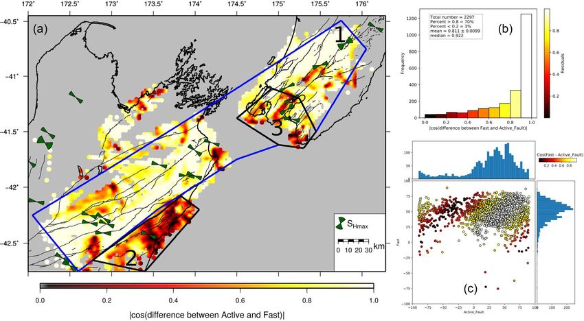
1996       K.M. Graham et al.

                                                                                                                                                                   Downloaded from https://academic.oup.com/gji/article/223/3/1987/5904048 by guest on 17 October 2020
Figure 4. Rose diagrams (circular histograms) showing the φ orientation results from local S-phase events, φ. Rose diagrams are plotted on the stations at
which measurements were made with a basemap of the digital topography and bathymetry. The green bow ties shows the crustal SHmax orientations from
Townend et al. (2012) and Balfour et al. (2005) with wedges showing the 95 per cent confidence interval. The black lines are the active faults. The two red rose
diagrams are measurements from Audoine et al. (2000) showing bimodal distributions.

Figure 5. SWS fast orientation results from local S-phase events for before, A (from 01/01/13 to 13/11/16) and after, B (from 14/11/16 to 30/06/18) (bottom)
Kaikōura main shock. The φ orientation determined from events recorded at each station are represented as rose diagrams and plotted on a basemap of the
digital topography. Rose diagrams are plotted on the stations at which measurements were made. The green bow ties shows the SHmax orientations from
Townend et al. (2012) and Balfour et al. (2005) with wedges showing the 95 per cent confidence interval. The blue lines are the faults that ruptured during the
Kaikōura Earthquake (Langridge et al. 2016).
Spatiotemporal analysis of seismic anisotropy 1997
Downloaded from https://academic.oup.com/gji/article/223/3/1987/5904048 by guest on 17 October 2020
Figure 6. Spatial averages of fast polarization orientation with weighting inversely proportional to the square of the distance from the station. The bars are
coloured by the orientation of the mean φ. Black lines are known active faults from the NZ Active Faults Database and the green lines are the faults that
ruptured during the 2016 Kaikōura main shock (Litchfield et al. 2017).
5 DISCUSSION Savage 2013) where they reported delay times for SKS measure-
ment far greater than the observed local S-phase measurements.
5.1 Overall station trends Similarly most studies of SKS waves assume the mantle is the main
source of anisotropy (e.g. Savage 1999).
The observed delay times, varying between near 0 and 0.372 s, are
The bi-modal distribution of fast orientation measurements ob-
in agreement with other SWS studies of crustal earthquakes (Au-
served at stations TMWZ and MTW on the North Island (Fig. 4)
doine et al. 2000; Balfour et al. 2005; Crampin et al. 2015; Cochran
reinforces previous observations. Audoine et al. (2000) reported a
& Kroll 2015; Savage et al. 2016). Vp /Vs ratios varying from 1.58
similar bi-modal distribution of φ measurements at stations LKER
to 2.22 with an average of 1.746 ± 0.001, are also consistent with
and LKIR (red rose diagram on Fig. 4), which were in close prox-
tomography results from Eberhart-Phillips & Fry (2018) and close
imity to TMWZ and MTW. At station HOWZ, the dominant φ
to the global average of 1.76 for continental crust (Christensen
orientation is parallel to faulting in the area and also subparallel to
1996). There is however substantial variability in φ measurements
SHmax . The correlation between φ orientation and the active fault
(the standard deviation of the φ measurements is greater than 30◦ at
orientations at these stations suggests that the sources of anisotropy
most stations). The observed large scatter of φ measurements sug-
beneath them could be structurally controlled. However, the faults
gests that the source of anisotropy may be a combination of more
are also parallel to the strike of the topography, which is consistent
than one mechanism or that the mechanism varies rapidly spatially
with near surface gravitational stress. Fast orientations at stations
(Peng & Ben-Zion 2004). The significant spatial variation we ob-
WEL and TCW (on either side of the Cook Strait; Fig. 4) are
serve illustrates the complex regional tectonics and heterogeneous
consistent with recent studies (Balfour et al. 2005; Evanzia et al.
structures around central New Zealand.
2017) around the Marlborough and Wellington region. However,
The average δt we observed (Tables 1 and 2) is about 6–
they show neither an agreement with SHmax orientations, nor with
14 per cent of the values reported in SKS studies (∼1.6 s) around
tectonic structures in the region.
New Zealand (Klosko et al. 1999; Zietlow et al. 2014). This small
Around the Marlborough region, the faulting is mainly strike slip,
value of δt suggests that there is a deeper source of anisotropy
thus based on Anderson’s theory of faulting (Anderson 1905; Healy
beneath these stations that is measured by SKS and our measure-
et al. 2012), we expect the faults to generally strike at an angle of
ments see only shallow anisotropy. A similar conclusion has been
∼30◦ to the orientation of SHmax . Stations KHZ, IKR, CRF and GBR
reached by previous studies (Audoine et al. 2000; Karalliyadda &You can also read