Comprehensive bathymetry and intertidal topography of the Amazon estuary
←
→
Page content transcription
If your browser does not render page correctly, please read the page content below
Earth Syst. Sci. Data, 13, 2275–2291, 2021
https://doi.org/10.5194/essd-13-2275-2021
© Author(s) 2021. This work is distributed under
the Creative Commons Attribution 4.0 License.

        Comprehensive bathymetry and intertidal topography of
                       the Amazon estuary
                Alice César Fassoni-Andrade1,2 , Fabien Durand1,2 , Daniel Moreira3 , Alberto Azevedo4 ,
                         Valdenira Ferreira dos Santos5 , Claudia Funi5 , and Alain Laraque6
          1 Laboratoire d’Etudes en Géophysique et Océanographie Spatiales (LEGOS), Université Toulouse, IRD,
                                             CNRS, CNES, UPS, Toulouse, France
                       2 Institute of Geosciences, University of Brasília (UnB), Campus Darcy Ribeiro,

                                                   Asa Norte, Brasília, Brazil
                               3 CPRM, Serviço Geológico do Brasil, Urca, Rio de Janeiro, Brazil
                             4 Laboratório Nacional de Engenharia Civil (LNEC), Lisbon, Portugal
                       5 Instituto de Pesquisas Científicas e Tecnológicas do Estado do Amapá (IEPA),

                                           Campus IEPA Fazendinha, Macapá, Brazil
              6 IRD, GET-UMR CNRS/IRD/UPS – UMR 5562 du CNRS, UMR 234 de l’IRD, Toulouse, France

           Correspondence: Alice Fassoni-Andrade (alice.fassoni@gmail.com, alice.fassoni@legos.obs-mip.fr)

                                 Received: 27 January 2021 – Discussion started: 8 February 2021
                            Revised: 19 April 2021 – Accepted: 22 April 2021 – Published: 26 May 2021

       Abstract. The characterization of estuarine hydrodynamics primarily depends on knowledge of the bathymetry
       and topography. Here, we present the first comprehensive, high-resolution dataset of the topography and
       bathymetry of the Amazon River estuary, the world’s largest estuary. Our product is based on an innovative ap-
       proach combining spaceborne remote sensing data, an extensive and processed river depth dataset, and auxiliary
       data. Our goal with this mapping is to promote the database usage in studies that require this information, such as
       hydrodynamic modeling or geomorphological assessments. Our twofold approach considered 500 000 sounding
       points digitized from 19 nautical charts for bathymetry estimation, in conjunction with a state-of-the-art topo-
       graphic dataset based on remote sensing, encompassing intertidal flats, riverbanks, and adjacent floodplains. Fi-
       nally, our estimate can be accessed in a unified 30 m resolution regular grid referenced to the Earth Gravitational
       Model 2008 (EGM08), complemented both landward and seaward by land (Multi-Error-Removed Improved-
       Terrain digital elevation model, MERIT DEM) and ocean (General Bathymetric Chart of the Oceans version
       2020, GEBCO_2020) topographic data. Extensive validation against independent and spatially distributed data,
       from an airborne lidar survey, from ICESat-2 altimetric satellite data, and from various in situ surveys, shows
       a typical vertical accuracy of 7.2 m (riverbed) and 1.2 m (non-vegetated intertidal floodplains). The dataset is
       available at https://doi.org/10.17632/3g6b5ynrdb.2 (Fassoni-Andrade et al., 2021).

1   Introduction                                                   to energetic exchanges of momentum between the upstream
                                                                   river and the ocean, with a marked variability in the water
The Amazon River exports the largest discharge of fresh-           level over a broad range of timescales, from the semidiur-
water (205 000 m3 s−1 ; Callède et al., 2010) and the largest      nal tide propagating upstream from the Atlantic Ocean to the
sedimentary supply (5–13 × 108 t yr−1 ; Filizola et al., 2011)     interannual hydrometeorological climatic events frequently
worldwide. However, to date, no consistent, comprehensive,         occurring over the upstream catchment. These exchanges
publicly available topographic dataset has been available for      between the river and the ocean result in sporadic flood-
the estuary that can support hydrodynamic, sedimentary, or         ing events, which profoundly impact the riparian commu-
ecological studies. The largest estuary in the world is home

Published by Copernicus Publications.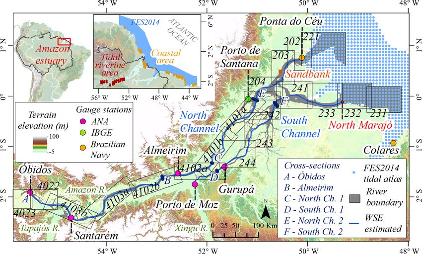
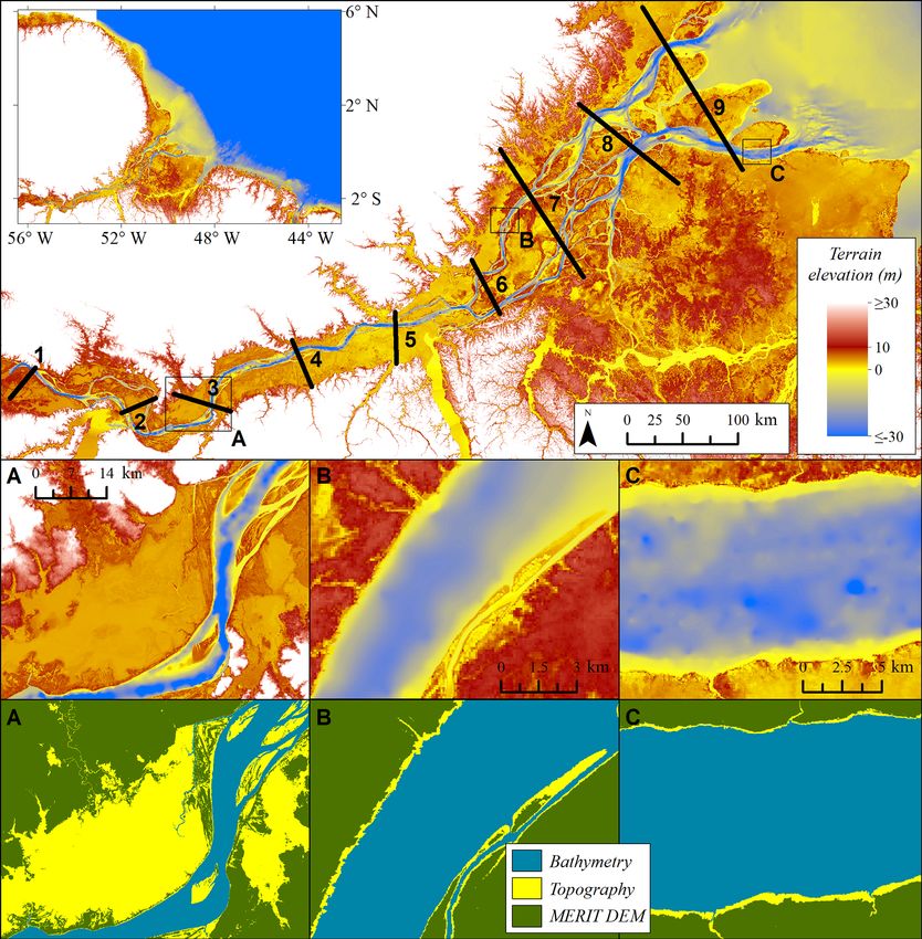
2276           A. C. Fassoni-Andrade et al.: Comprehensive bathymetry and intertidal topography of the Amazon estuary

Figure 1. Location of the Amazon River estuary, identifying and delimiting nautical charts (Brazilian Navy – black boxes) and showing
the locations of gauge stations of the Agência Nacional de Águas (ANA), the Brazilian Navy, and the Instituto Brasileiro de Geografia e
Estatística (IBGE). Terrain elevation from MERIT DEM.

nities’ socioeconomic conditions (Andrade and Szlafsztein,            (Kosuth et al., 2009). Thus far, the quantitative investigation
2018; Mansur et al., 2016). The morphology of the riverbed            of the estuary’s hydrodynamics and the interaction mecha-
is known to primarily condition the estuary’s hydrodynam-             nisms between the tide and the river flow has been limited by
ics, particularly the propagation of the tidal wave (Gallo and        the lack of sufficiently resolved bathymetric databases (e.g.,
Vinzon, 2015), which is expected to affect the dynamics of            Gabioux et al., 2005). Therefore, past hydrodynamical stud-
the riverine floods and the extent of the associated flooding         ies of the Amazon estuary relied on approaches based on box
(Kosuth et al., 2009). This dynamic environment with high             models (Prestes et al., 2020) and/or on coarse hydrodynam-
ecological diversity is essential for nutrient cycling and car-       ical models (e.g., Gallo and Vinzon, 2015). Still, these past
bon fluxes (Sawakuchi et al., 2017; Ward et al., 2015), for           studies revealed rich hydrodynamics of the estuary, compris-
navigation (Fernandes et al., 2007), and for the transport and        ing contrasting patterns of bottom friction (Gabioux et al.,
accumulation of sediment (Nittrouer et al., 2021).                    2005), active nonlinear deformation of the tidal waves (Gallo
   The Amazon estuary extends from the continental shelf              and Vinzon, 2005), a distinct structure of the salinity front
up to Óbidos city, corresponding to the longest tidally influ-        (Molinas et al., 2014, 2020), and a prominent role of the in-
enced reach in the world, extending over 800–910 km (Ko-              tertidal flats in the flow variability (Gallo and Vinzon, 2005).
suth et al., 2009; Nittrouer et al., 2021; Fig. 1). This river        The interplay between the fluvial variability in the water level
flow is drained downstream towards the ocean through the              and its tidal variability is particularly known to exert a cen-
main channel until the confluence with the Xingu River,               tral control on the estuary’s sedimentation pattern (Fricke
around 300 km upstream of the mouth, where it is divided              et al., 2019). While the geometry of the Amazon estuary is
into two long channels, hereafter called “South Channel” (lo-         known to have been influenced little by anthropogenic effects
cally named Gurupá Channel) and “North Channel” (Fig. 1).             to date, it appears essential to document it in its current state,
Downstream of this branching, the estuary appears as a com-           at a time when the human influence is rising and is expected
plex network of dendritic tidal channels and islands (Fricke          to induce profound, long-lasting impacts on the continental
et al., 2019). The estuary is classified as macrotidal (Dyer,         sediment supply to this estuary (Latrubesse et al., 2017).
1997; Gallo and Vinzon, 2005) and semidiurnal (Kosuth                    The present paper aims to present a novel topographic and
et al., 2009) with a tidal range between 4 and 6 m at the             bathymetric dataset of the whole Amazon River estuary, from
mouth. The M2 (lunar semidiurnal) and S2 (solar semidi-               its upstream limit 1000 km inland to its terminal estuary at its
urnal) tidal constituents are the dominant components at the          oceanic outlet, covering the riverbed as well as the intermit-
ocean boundary, with respective amplitudes of 1.5 and 0.4 m           tently flooded riverbanks and adjoining floodplains. Over the
there (Gallo and Vinzon, 2005). At the upstream limit of              continually wet part of the riverbed, we rely on a traditional
the estuary in Óbidos, the range of the drought–flood annual          methodology to construct the bathymetry based on compre-
cycle of the river height typically amounts to 6 m, and the           hensive, systematic digitization of existing nautical charts. In
tidal effects remain detectable only during the drought season        contrast over the intermittently dry intertidal zones and flood-

Earth Syst. Sci. Data, 13, 2275–2291, 2021                                             https://doi.org/10.5194/essd-13-2275-2021
A. C. Fassoni-Andrade et al.: Comprehensive bathymetry and intertidal topography of the Amazon estuary                      2277

plains, our mapping is achieved through an original, state-of-     of the low tide during spring tides for SYZ. These references
the-art approach based on spaceborne remote sensing. Our           were computed with respect to the geoid considering the
dataset is regularly gridded at a 30 m resolution and eleva-       absolute leveling published in Calmant et al. (2013) and
tions are referenced to the Earth Gravitational Model 2008         Callède et al. (2013), complemented by a dedicated geodetic
(EGM08; Pavlis et al., 2012). It covers the river streams,         field survey that we conducted in January–February 2020
riverbanks, and floodplains, and it extends downstream of          (Appendix A). At the river mouth, downstream of the
the estuary mouths over the near-shore ocean shelf and open-       downstream-most tidal stations (blue points in Fig. 1), the
ocean coastline, covering the domain shown in Fig. 1.              SYZ level was calculated using a combination of the mean
   The remainder of the paper is structured as follows: Sect. 2    sea surface height provided by the ocean general circula-
presents the data sources and the methods used to build the        tion model of Ruault et al. (2020) and of a proxy of the
dataset; Sect. 3 presents the validation against independent       syzygy level estimated by the FES2014 tidal atlas (Carrère
databases; Sect. 4 shows the topographic mapping and cross         et al., 2016; available at https://www.aviso.altimetry.fr/
section along the river and floodplain; Sect. 5 discusses the      en/data/products/auxiliary-products/global-tide-fes.html,
significance and caveats of the dataset; and Sect. 6 explains      last access: 1 November 2020). This proxy for SYZ was
the access to the various forms of our dataset.                    defined classically according to Eq. (1), from the sum of the
                                                                   amplitudes of the M2 and S2 tidal constituents (Pugh and
                                                                   Woodworth, 2014):
2     Data and methods
                                                                   SYZ = mean sea surface height − (M2 + S2).                 (1)
2.1    Bathymetry of the riverbed
                                                                      We inferred the WSE (i.e., WS90 or SYZ, depending on
Over the continually wet part of the various streams of            the reference of the chart under consideration) separately
the Amazon estuary, the approach relies on systematic              along the Amazon River (Óbidos, Santarém, and Almeirim),
digitization of sounding points of bed elevation harvested         the North Channel (Porto de Santana and Ponta do Céu),
from a comprehensive ensemble of nautical charts pub-              and the South Channel (Almeirim, Porto de Moz, Gurupá,
lished by the Brazilian Navy (available at https://www.            and a point of the FES2014 tidal model marked as “North
marinha.mil.br/chm/dados-do-segnav/cartas-raster, last ac-         Marajó” in Fig. 1) via linear interpolation between the suc-
cess: 29 July 2020). Although technically straightforward,         cessive stations, resulting in the profile shown in Fig. 2c.
this task was by far the most tedious part of the procedure,       The linear interpolation considered successive points along
on account of the large geographical extent of the domain          the river spaced by 30 m and represented by the two blue
(21 500 km2 , gray polygon in Fig. 1). We digitized more than      lines in Fig. 1. The WSE for each of the 500 000 digitized
500 000 individual points from a total of 19 charts, which are     points was then inferred from the values along the river
identified and delimited in Fig. 1. The primary bathymetric        via a nearest-neighbor interpolation method. Following this,
surveys utilized in these charts were carried out by the Brazil-   the WSE was subtracted from the water depths, resulting in
ian Navy on different dates varying between 1953 and 2019,         bed elevation values referenced to EGM08. The bed eleva-
with a reasonably large fraction of them done after 2000 (see      tion points were then interpolated using the “topo-to-raster”
Table A1 for further details). Figure 2a displays an example       method (Hutchinson, 1989), which is essentially an interpo-
of a digitized nautical chart. One issue with the maps that we     lation method suited to hydrological objects to create a regu-
could access was the vertical referencing of the digitized ele-    lar elevation grid with a 30 m spatial resolution.
vations. Depending on the map considered, the bed elevation           In the interpolation, a river boundary was considered, as
values were provided with respect to two different reference       shown in Fig. 1 (gray polygon) and exemplified in Fig. 2b
water surface elevations (WSEs): either the level of the 90th      (bathymetric boundary). This boundary is a polygon defined
percentile of water surface elevation (hereafter referred to as    considering a flood frequency of between 96 % and 100 %.
WS90) or the average level of the low tide during the spring       The flood frequency map was calculated from the Global
tide (termed syzygy and hereafter referred to as SYZ).             Surface Water (GSW) Monthly Water History v1.2 data
   We inferred the vertical elevation of each of these two         (Pekel et al., 2016; available at https://global-surface-water.
references from the available records of the tide gauge            appspot.com, last access: 3 August 2020), which represents
stations scattered along the river down to the river mouth.        the spaceborne Landsat-based monthly record of water pres-
The tidal and limnigraphic records from the seven stations         ence on a global scale with a spatial resolution of 30 m. A
that we could access, listed in Tables A2 and A3 (locations        Google Earth engine code (Gorelick et al., 2017), described
in Fig. 1), were provided by the Agência Nacional de Águas         in Fassoni-Andrade et al. (2020b), was used to create the
(ANA), the Brazilian Navy, and the Instituto Brasileiro de         flood frequency map and considered all GSW monthly im-
Geografia e Estatística (IBGE). The vertical water level of        ages from the period from January 2015 to December 2018,
both references (WS90 and SYZ) was deducted explicitly             resulting in a total of 48 months. This 48-month period was
from the temporal records by computing the level of the 90th       found to be a good compromise between a short enough pe-
percentile to infer WS90 and by computing the average level        riod to ensure that the dataset was recent enough and a long

https://doi.org/10.5194/essd-13-2275-2021                                         Earth Syst. Sci. Data, 13, 2275–2291, 2021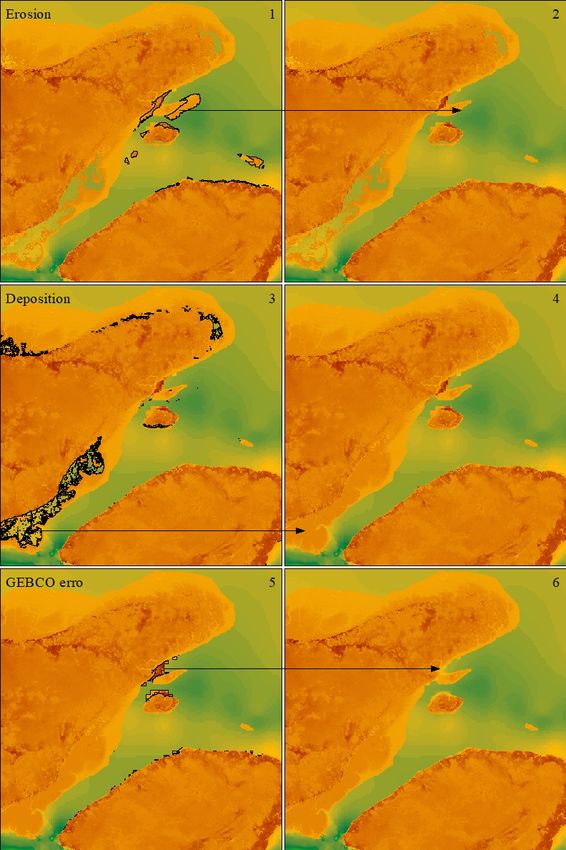
2278            A. C. Fassoni-Andrade et al.: Comprehensive bathymetry and intertidal topography of the Amazon estuary

                                                                       coastal topography pixel by pixel (Armon et al., 2020; Dai et
                                                                       al., 2019; Tseng et al., 2017). In these approaches, reference
                                                                       water levels (for instance, minimum, average, and maximum)
                                                                       were assigned to reference flood frequencies (100 %, 50 %,
                                                                       and 0 %, respectively). In contrast to these approaches that do
                                                                       not explicitly require knowledge of the water level’s temporal
                                                                       variation, Fassoni-Andrade et al. (2020b) related the function
                                                                       of water level exceedance probability and a flood frequency
                                                                       map to estimate the topography of the water bodies. The au-
                                                                       thors showed that the terrain elevation for a given pixel is
                                                                       defined as the water level, whose probability of exceedance
                                                                       is equal to the flood frequency there. Figure 3 exemplifies the
                                                                       method.
                                                                          This straightforward approach requires a flood frequency
                                                                       map and the water level exceedance probability functions to
                                                                       generate the terrain elevation map (Fig. 3). It has been ap-
                                                                       plied in situations where the temporal dynamics of water fill-
                                                                       ing and draining is slow. Here, the same method is applied to
                                                                       estimate the floodplain topography and coastal topography
Figure 2. (a) Example of a nautical chart near the river mouth (code
                                                                       of the Amazon estuary, where the water level variability is
233). (b) Digitized pointwise soundings and isobaths, along with
bathymetric boundaries (defined as the 96 % isoline of flood fre-
                                                                       spread over a broader spectrum, from intra-daily timescales
quency) and topographic boundaries (defined as the 0 % isoline of      to seasonal or interannual timescales (Kosuth et al., 2009).
flood frequency); the two regions are immediately adjacent. (c) Ref-   As we did not have access to vertically leveled tide gauge
erenced WSE (black lines) and average WSE (blue lines) along the       archives in the Amazon estuary coastal area, two domains
Amazon estuary (EGM08 geoid).                                          were considered for topography estimation (Fig. 3). The first
                                                                       domain considered the riverbanks, intertidal zone, and flood-
                                                                       plains along the channels (described in Sect. 2.2.1), where
enough period that it was capable of capturing the bulk of the         the approach described in Fassoni-Andrade et al. (2020a)
flooding statistics.                                                   was directly applied. Downstream of the estuary mouths,
                                                                       over the open near-shore Atlantic Ocean, the method was
2.2    Topography of periodically flooded areas
                                                                       adapted to estimate tidal variation considering the water level
                                                                       exceedance function from a tidal station (Sect. 2.2.2).
Intertidal banks and floodplains are areas periodically
flooded by tides and riverine floods, respectively. We de-             2.2.1   Riverbanks, intertidal zone, and floodplains
fine them as the areas comprising between 0 % and 96 %
of the abovementioned flood frequency map. In past stud-               In the intertidal zone and floodplains along the Amazon
ies devoted to coastal mapping, intertidal topography has              River, WSE records from limnigraphic and tidal stations
been mapped using remote sensing data, with the waterline              were considered over the period from 2015 to 2018 (Ta-
method being one of the most widely adopted techniques                 bles A2 and A3) for consistency with the imagery period
(see Salameh et al., 2019, for a review). This method re-              covered by the flood frequency map. These records yielded
quires the detection and extraction of the water contours in           exceedance probability functions, such as the one illustrated
imagery time series. Next, water levels are assigned to the            in Fig. 4b (Óbidos station). Like WSE estimation along the
individual water contours, creating isobaths. A digital ele-           river (Sect. 2.1), the water level duration curve was inferred
vation model (DEM) raster can be generated from a large                separately along the North Channel and the South Channel
enough amount of such isobaths. Some recent applications               (blue lines in Fig. 1) by linearly interpolating the curves ob-
of this method are found in Bell et al. (2016), Bergmann et            tained at each station. The water level duration curves were
al. (2018), Bishop-Taylor et al. (2019), Khan et al. (2019),           then extrapolated via a nearest-neighbor interpolation over
and Salameh et al. (2020). This method has proven tractable            the estuary’s intertidal areas and floodplains, i.e., everywhere
with moderate-resolution spaceborne imagery; however, it               upstream estuary mouths. Therefore, the terrain elevation
requires simultaneous water level knowledge at the exact               for any pixel was estimated considering the water level, for
time of each acquisition, along the remotely sensed water-             which the probability of exceedance is equal to the flood fre-
lines. It also relies on spatial interpolation of the isobaths         quency for the same pixel (Fassoni-Andrade et al., 2020b).
between successive waterlines, which can be problematic if             In permanently flooded areas, i.e., where the flood frequency
the waterlines are sparse. Recently, alternative methods have          is 100 %, the method considers the topography equal to the
been developed using a flood frequency map to estimate the             lowest WSE observed, as in the river.

Earth Syst. Sci. Data, 13, 2275–2291, 2021                                             https://doi.org/10.5194/essd-13-2275-2021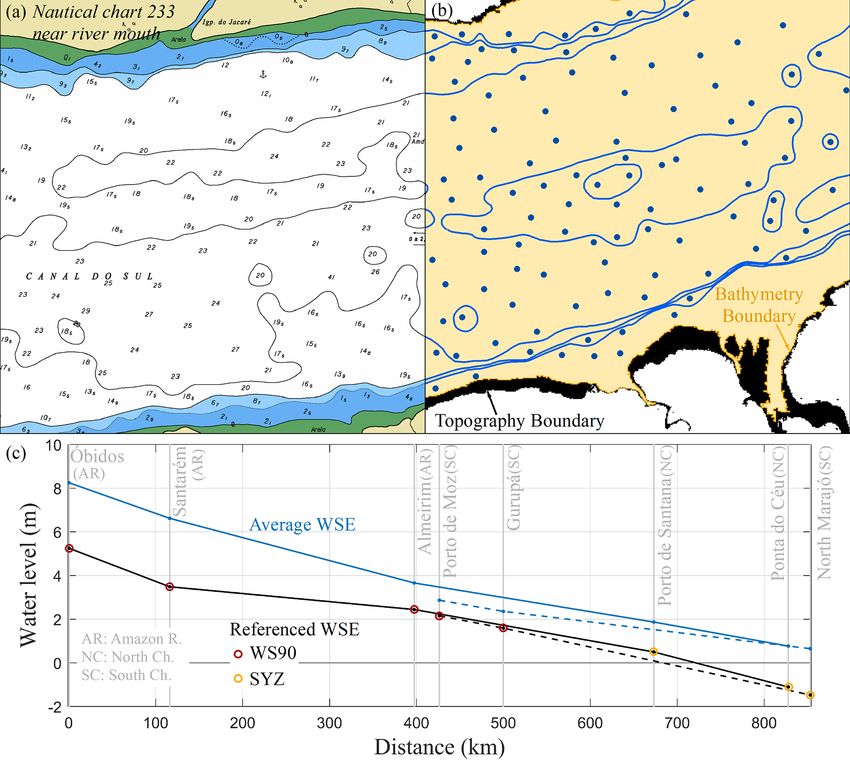
A. C. Fassoni-Andrade et al.: Comprehensive bathymetry and intertidal topography of the Amazon estuary                                 2279

Figure 3. Method to estimate the topography of the water bodies (Fassoni-Andrade et al., 2020b; left panel) and the various datasets
considered in this study to implement this method (right panel).

Figure 4. (a) Close-up view of the flood frequency map over the Amazon estuary’s upstream area. (b) The water level duration function
at Óbidos station. (c) The observed and estimated water level duration function at Colares station. (See Fig. 1 for the location of these two
stations.)

2.2.2   Coastal ocean                                                    Amazon estuary station of Ponta do Céu (Table A2; location
                                                                         in Fig. 1) and computed the water level exceedance function
The challenge with respect to estimating the topography in               there. This curve’s shape was then assumed to be the same
the coastal area using the methodology of Fassoni-Andrade                throughout the coastal region, although with variable ampli-
et al. (2020b), where vertically leveled tide gauges are lack-           tude, proportional to the local tidal amplitude. In this semid-
ing, is the inference of spatially distributed water level ex-           iurnal macrotidal region, a reasonable proxy of the tidal am-
ceedance functions. We considered the downstream-most                    plitude over the region can be thought of as the sum of the

https://doi.org/10.5194/essd-13-2275-2021                                                Earth Syst. Sci. Data, 13, 2275–2291, 2021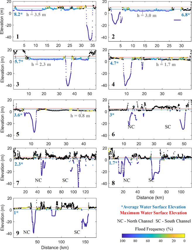
2280            A. C. Fassoni-Andrade et al.: Comprehensive bathymetry and intertidal topography of the Amazon estuary

amplitudes of the S2 and M2 tidal constituents, as these two      2.3.2   Ice, Cloud, and land Elevation Satellite-2
constituents are the dominant ones downstream of the river                (ICESat-2) spaceborne data
mouth (Gallo and Vinzon, 2005). The water level duration
                                                                  The topography was further validated against Ice, Cloud,
function (WLDF) at any point along the oceanic coastline
                                                                  and land Elevation Satellite-2 (ICESat-2) data. Launched in
was obtained by scaling the corresponding function observed
                                                                  September 2018, the satellite provides measurements of the
at Ponta do Céu (WLDFPC ) considering the tidal amplitude
                                                                  surface level from the transmission of laser pulses in the
given by the S2 and M2 components from the FES2014
                                                                  green wavelength (532 nm) by the Advanced Topographic
model (Carrère et al., 2016), according to Eq. (2):
                                                                  Laser Altimeter System (ATLAS) instrument. ATLAS beams
                          tidal amplitude                         provide six tracks, divided into three pairs, on the Earth sur-
WLDF = WLDFPC ×                           ,                (2)    face along the ICESat-2 orbit. The beam pairs are separated
                        tidal amplitudePC
                                                                  by ∼ 3.3 km in the across-track direction, and each spot on
where the tidal amplitude at a point is given by 2×(S2+M2),       the surface has a ∼ 13 m footprint diameter (Neuenschwan-
and the PC subscript refers to Ponta do Céu values.               der et al., 2020). The accuracy expected from ATLAS is ap-
   As verification, Fig. 4c shows the observed and estimated      proximately 25 cm for flat surfaces and 119 cm in the case of
exceedance probability functions at Colares station, located      a 10◦ surface slope (Neuenschwander et al., 2020).
about 150 km to the east of the Amazon estuary (Fig. 1). Both        The ATL08 version 3 dataset, derived from ATLAS mea-
curves represent the anomaly with respect to the average. The     surements, provides along-track heights above the WGS84
two curves look very similar, with a root-mean-square devi-       ellipsoid for the land and vegetation every 100 m (available
ation (RMSD) of 12.7 cm.                                          at https://nsidc.org/data/ATL08, last access: 3 August 2020).
   After estimating the water level exceedance probability at     ATL08 data can also represent water surface elevation; there-
each point, the vertical reference was adjusted by matching       fore, a criterion has been used to separate these from the
the mean level with the height of the mean sea surface esti-      measurements over the land surface. Some studies have also
mated by the ocean circulation model of Ruault et al. (2020).     shown that the ATLAS instrument can penetrate water and
Similar to the water level exceedance probability functions       provide information on the bottom (Ma et al., 2020; Parrish
estimated along the river, the coastal area’s water level du-     et al., 2019). As the Amazon River has a high concentration
ration functions were inferred for all pixels of the flood fre-   of sediments (Martinez et al., 2009), we assume that target
quency map considering the nearest-neighbor interpolation         information from the water only represents the water surface
method. Therefore, the terrain elevation for a pixel was esti-    elevation.
mated considering the water level, for which the probability         Two regions were selected for the validation of topogra-
of exceedance is equal to the flood frequency for the same        phy: upstream of the Xingu River, where the tidal amplitude
pixel (Fassoni-Andrade et al., 2020b).                            is small (∼ 40 cm; Kosuth et al., 2009), and along the oceanic
                                                                  coastal area (see Fig. 1 inset map for the locations of both
                                                                  of these regions: “Tidal riverine area” and “Coastal area”,
2.3     In situ and spaceborne data for validation                respectively). In both regions, cloudy conditions and mea-
                                                                  surements with uncertainty above 50 cm (as indicated by the
2.3.1    Governo do Estado do Amapá and Exército                  dataset flags) were discarded. Criteria to remove the points
         Brasileiro (GEA/EB) digital terrain model                derived from the water elevation were considered in each
                                                                  case. In the tidal riverine region, only ATL08 points, con-
A digital terrain model (DTM) with a 2.5 m spatial reso-
                                                                  verted to EGM08 heights, from the October–December sea-
lution and an accuracy of 1.62 m (BRADAR, 2017), pro-
                                                                  sons of 2018 and 2019 were considered, as this period repre-
vided by the Instituto de Pesquisas Científicas e Tecnológ-
                                                                  sents the low-water season of the Amazon River. Moreover,
icas do Estado do Amapá (IEPA; http://www.iepa.ap.gov.br/,
                                                                  as the flooded areas should show very low variability in the
last access: 27 January 2021), was used to validate the esti-
                                                                  spaceborne measurements along the track, it is easy to detect
mated topography on a sandbank covering ∼ 0.9 km2 in the
                                                                  them in the individual along-track data. Thus, each track’s
North Channel (location in Fig. 1). This area was chosen
                                                                  water level was evaluated, and points below 50 cm above the
because it is an almost non-vegetated area and it has suf-
                                                                  water elevation were discarded. For the coastal area, tracks
ficient corresponding topographic mapping points. For con-
                                                                  with a visually markedly different elevation between ocean
sistency, the DTM vertical reference was transformed from
                                                                  and continent were selected. Each selected track was evalu-
MAPGEO2010 (Matos et al., 2012) to EGM08. The DTM
                                                                  ated, and points below 1 m above the water elevation were
was developed using P-band interferometry from an aerial
                                                                  discarded.
survey conducted in late 2014 and early 2015 (De Castro-
Filho and Antonio Da Silva Rosa, 2017) in the context of
the Base Cartográfica Continua do Amapá project (Vieira,
2015) in cooperation with Governo do Estado do Amapá and
Exército Brasileiro (GEA/EB).

Earth Syst. Sci. Data, 13, 2275–2291, 2021                                        https://doi.org/10.5194/essd-13-2275-2021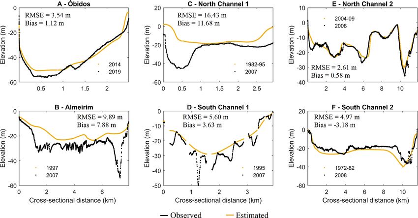
A. C. Fassoni-Andrade et al.: Comprehensive bathymetry and intertidal topography of the Amazon estuary                     2281

2.3.3    In situ surveys of the riverbed bathymetry              wiping out staircases artifacts. Moreover, a low-pass filter
                                                                 with a 9 point × 9 point and 19 point × 19 point window
The riverbed was evaluated in six different bathymetry cross     moving average (i.e., 4.5 km × 4.5 km and 9.5 km × 9.5 km,
sections acquired from past in situ surveys carried out over     respectively) was used in the respective regions above
the 2007–2019 period by SO HYBAM (see https://hybam.             (shoreward) and below (off- shoreward) the −200 m isobath
obs-mip.fr/, last access: 27 January 2021) and Companhia         to reduce the noise caused by in situ multibeam sounding
de Pesquisa de Recursos Minerais (CPRM; location of cross        swaths edges.
sections in Fig. 1). The water depth was obtained by an             These combined databases allowed a unified mapping of
acoustic Doppler current profiler (ADCP) instrument, and a       the topography and bathymetry of the Amazon estuary. How-
WSE was considered here for estimating the bed elevation         ever, as MERIT DEM represents the topography of 2010 and
concerning EGM08. In Section A, we considered the WSE            some areas in the coastal region may have been eroded or
at Óbidos station on the survey day (28 November 2019).          accreted between 2010 and the 2015–2017 period consid-
In sections, B, C, and D, the WSE at Porto de Moz station        ered in the flood frequency mapping, a procedure was im-
on the day of the survey was used and was corrected for          plemented to correct this issue considering three types of
each section taking the water surface declivity obtained by      regions: (1) erosion areas; (2) accretion areas, i.e., regions
the WSE estimated along the river (Fig. 2c) and the distance     where MERIT product does not have topographic informa-
between the station and section, i.e., WSE at section = WSE      tion; and (3) GEBCO regions that represent the continent
at Porto de Moz + WSE slope × distance, into consideration.      due to sparse spatial resolution, whereas it should repre-
Finally, the WSE measured every 15 min at Porto de Santana       sent transition areas or the ocean. The procedure was per-
station on 5 June 2008 was considered in sections E and F.       formed as follows: (1) MERIT DEM areas with topographic
As the water level varied by ∼ 50 cm during the time span of     information in eroded areas were selected and replaced by
these sections, described in Callède et al. (2010), the high-    GEBCO data, which cover both the continent and the ocean.
frequency WSE at each point of the sections was considered.      In the case of substitution to continent GEBCO data, the re-
Furthermore, metrics were evaluated considering all points       gion was corrected again in step three. (2) Deposition areas
(excluding outliers) in the round-trip survey and repetitions.   where MERIT does not have topographic information were
In Section A, four cross sections were acquired; in sections     estimated from the topo-to-raster interpolation method con-
B, C, and D, only one cross section was obtained; and in         sidering the values in the mapped regions’ contours. Simi-
sections E and F, six and nine cross sections were obtained,     larly, (3) GEBCO’s high topographic regions in the ocean,
respectively.                                                    including regions not previously corrected in step one, were
                                                                 removed, and new values were estimated by topo-to-raster
2.4     Ancillary databases                                      interpolation considering the neighboring pixels. These ar-
                                                                 eas were manually selected considering the polygons gen-
The estimated topography does not cover the terrain el-          erated from the elevation reclassification into three classes
evation in the non-open-water area. Similarly, our set of        (visually defined criteria): less than −8 m, between −8 and
bathymetric charts does not cover the Atlantic Ocean’s           1 m, and greater than 1 m. Figure A1 shows an example of
continental shelf downstream of the river mouth. Thus,           these steps and a corrected area. Finally, to ensure a smooth
our dataset was complemented by two global databases:            transition between the nautical charts and GEBCO, an area
the Multi-Error-Removed Improved-Terrain (MERIT)                 was selected and replaced considering topo-to-raster inter-
DEM over the continental area and General Bathymetric            polation from the neighboring pixels. This area was defined
Chart of the Oceans (GEBCO) version 2020 over the                by a buffer of ∼ 2 km around the transition limit, i.e., consid-
ocean. MERIT DEM is a widely used global model with              ering 4 km width.
a spatial resolution of 90 m in which several errors of the
Shuttle Radar Topography Mission (SRTM) DEM and
                                                                 3     Validation
the height of vegetation have been corrected (available
at http://hydro.iis.u-tokyo.ac.jp/~yamadai/MERIT_DEM/;           3.1    Topography
Yamazaki et al., 2019). For consistency, the MERIT DEM
reference was changed from EGM96 to EGM08 (Pavlis                Figure 5 shows the validation of the estimated topography
et al., 2012). GEBCO is a global terrain model referred          considering the GEA/EB DTM (“Sandbank” label in Fig. 1)
to mean sea level with a spatial resolution of 15 arcsec         and the ICESat-2 data. The estimated elevation yields an
(approximately 460 m in the Amazon estuary; available            root-mean-square error (RMSE) of 1.15 m, a bias of −0.78 m
at       https://www.gebco.net/data_and_products/gridded_        (standard deviation, SD, of 0.85 m), and a Pearson correla-
bathymetry_data/gebco_2020/, last access: 1 Novem-               tion coefficient (r) of 0.52 (the number of data, n, was 612)
ber 2020). As GEBCO data have integer values at intervals        compared with GEA/EB DTM. This error may be partly re-
of 1 m, the topo-to-raster interpolation was used considering    lated to the spatial resolution of the Landsat images (30 m)
the 1 m isolines to generate data consistent with float values   and geomorphological changes in the island during 2014 and

https://doi.org/10.5194/essd-13-2275-2021                                       Earth Syst. Sci. Data, 13, 2275–2291, 2021
2282 A. C. Fassoni-Andrade et al.: Comprehensive bathymetry and intertidal topography of the Amazon estuary
2015, as shown in Fig. 5a and b. Still, this error is lower than of a channel from a wavy bedform during rising discharge
the DTM intrinsic accuracy (RMSE of 1.62 m). (January 1994) to a flat floor during low discharge (Novem-
Considering the ICESat-2 data, the terrain elevation was ber 1994) with a reduction of up to 7 m in the channel depth
also well represented in the riverbanks/floodplain and coastal (Vital et al., 1998). Therefore, accurate riverbed mapping of
area, with an r value of 0.8 and 0.8, a RMSE of 1.5 m and 1.8, this region remains challenging.
and a bias of 0.9 m and −1.5, respectively. However, Fig. 5f
shows a bias related to the flood frequency in which overes- 4 Topographic variation along the estuary
timations are observed at low flood frequencies (e.g., ∼ 3 m
for flood frequency of 0 %). As shown in Fassoni-Andrade et Figure 7 shows the resulting topography and bathymetry, as
al. (2020a), this bias may be related to the Landsat images well as the complementary MERIT DEM and GEBCO data.
used in the flood frequency map that do not represent the The extensive floodplain, riverbanks, and intertidal zone have
flood extent in flood-prone vegetated areas. Thus, the flood been seamlessly mapped, as exemplified in boxes A, B, and
frequency in these areas is considered only from situations C. It can be noted that the floodplain extent decreases from
when the water level exceeds the vegetation height; hence, the upstream area to the downstream area, and the chan-
the flood frequency is underestimated, mechanically overes- nels become dendritic in the eastern half of the estuary (east
timating the terrain elevation. of 52◦ W). This is related to the accumulation of sediment
and the fluvial and tidal influences, as described in Fricke et
3.2 Bathymetry al. (2019) and Nittrouer et al. (2021). These authors showed
that the upper estuary, characterized by low tidal influence
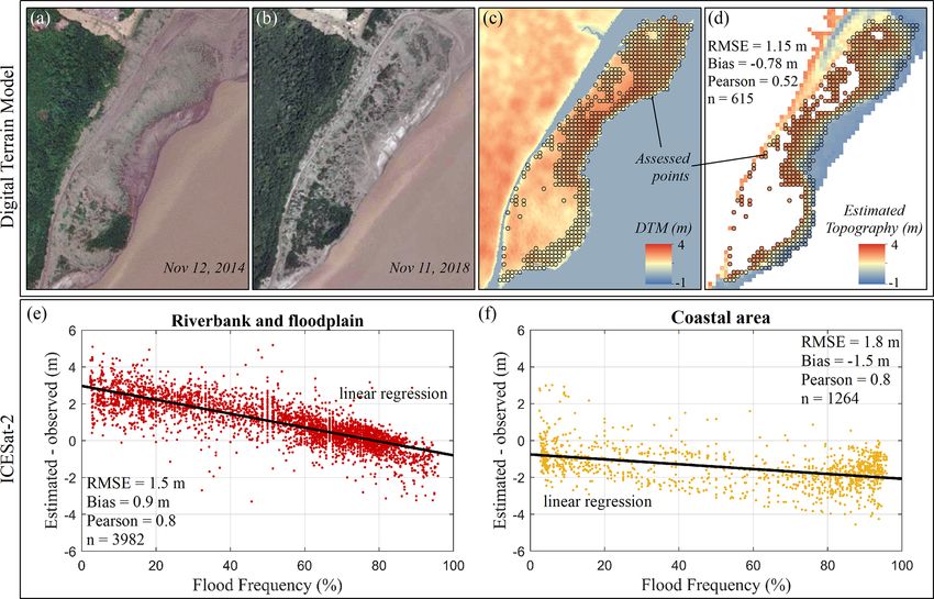
Figure 6 shows the comparison between the in situ cross sec- (∼ 40 cm or less), has high levees that limit the overbank flow
tions of the Amazon River and our product. The Amazon and sediment accumulation on the floodplain. In the central
River’s bed elevation was well represented, with an average reach, the stronger tidal range (∼ 1–2 m) and the associated
vertical RMSE of 7.2 m and an average bias of 3.6 m (SD tidal flow suppress the levees’ heights, inducing strong over-
of 5.38 m) for the six sections considered together. Keep- bank transport with high sedimentation rates on the flood-
ing aside the small-scale (typically sub-kilometric) features plain. In the lower reach with an even stronger tidal range
not resolved by the coarser bathymetric digitized charts, the (∼ 4 m), river-canalized transport predominates, and there is
shape of the cross sections appear appropriately captured by little space for sediment accumulation on the floodplain.
our product, along the steep banks as well as in the median In general, our product stands under this known geomor-
part. The smallest errors are observed in Óbidos (Section A; phological characterization, which is shown in the nine rep-
RMSE of 3.5 m) and North Channel 2 (Section E; RMSE of resentative topographic profiles in Fig. 8 (extracted in the
2.6 m), possibly due to the shorter time lag between the dates across-river direction every 100 km). The color bar repre-
of the surveys (< 5 years) and variation in the bed bathymetry sents the flood frequency from the GSW data, i.e., regions
(Vital et al., 1998). Section E, near Macapá city, is over a where topography and bathymetry were estimated. Black
broad area of overconsolidated sediments, which are difficult dots represent the MERIT DEM, and the horizontal lines rep-
to dredge (Vital et al., 1998). Furthermore, the WSEs consid- resent the average (blue) and the maximum (red) river WSE
ered in these sections are from nearby stations, reducing the (2015–2018). Note that the difference between the average
vertical reference uncertainties. WSE and the floodplain elevation tends to decrease from
On the other hand, although the in situ survey for South Section 1 to Section 5 (h values in gray); that is, the space
Channel 2 is about 40 years old (1972–1982; Section F), for sediment accommodation on the floodplain decreases due
good agreement appears with the SO HYBAM survey in to sediment accumulation. It can also be observed that the
2008 (RMSE of 5 m), which shows that the bed surface has height of the levees is similar to the maximum WSE in sec-
possibly not changed much in these 26–36 years. tions 1 to 5 (upper and central reach), but from Section 6 and
The region near the Almeirim station, i.e., sections B, C, further downstream, the topography, represented by the black
and D, seems to have undergone the most significant bed points, is higher than the maximum elevation and the river
change. In general, the errors are larger (e.g., RMSE of 16 m has no flooded banks. This observation in the estuary’s lower
in Section C), and the topographic variation was not repre- reach has more uncertainty because it considers the MERIT
sented in the nautical charts. The respective impact of the DEM data (Yamazaki et al., 2019), which were not validated
limited spatial resolution of the digitized nautical charts and here. Fricke et al. (2019) did not observe levees in this reach
of the morphological variability in the bed on the mismatch and described the topography as a flat surface, but the eval-
that we observe is not able to be clearly established in the uation of the authors considered topographic surveys of the
absence of additional information. These are areas of in- banks with a distance from the river of 30–250 m (average of
tense sediment transport with erosion and/or deposition of 80 m), which is equivalent to approximately three points of
sand and high variability in the riverbed morphology (Vital our analysis (30 m of spatial resolution).
et al., 1998). Marked seasonal changes in the riverbed were
reported due to extreme net erosion, such as the modification
Earth Syst. Sci. Data, 13, 2275–2291, 2021 https://doi.org/10.5194/essd-13-2275-2021A. C. Fassoni-Andrade et al.: Comprehensive bathymetry and intertidal topography of the Amazon estuary 2283 Figure 5. Sandbank represented by GEA/EB DTM and topographic mapping (location in Fig. 1). Panels (a) and (b) represent true-color images of the area from Landsat. Panel (c) shows GEA/EB DTM, and panel (d) shows the estimated topography. Flood frequency versus error in topographic estimation in (e) the riverbank/floodplain (“Tidal riverine area” in Fig. 1) and (f) the coastal area (“Coastal area” in Fig. 1) considering the ICESat-2 data. Figure 6. Cross-sectional transects of the Amazon River (locations are shown in Fig. 1) from the cross section estimated (yellow) and observed from the in situ surveys (black). Elevations are relative to EGM08. The dates of the corresponding in situ surveys are indicated in each panel. https://doi.org/10.5194/essd-13-2275-2021 Earth Syst. Sci. Data, 13, 2275–2291, 2021
2284            A. C. Fassoni-Andrade et al.: Comprehensive bathymetry and intertidal topography of the Amazon estuary

Figure 7. Unified topographic mapping of the Amazon estuary (referenced to EGM08): the bathymetry, topography, MERIT, and GEBCO
products were merged. The middle row displays close-up views of selected regions. The bottom row indicates the sources of the raw data for
the various subdomains.

5    Data availability                                                        DEM_AMestuary.nc) – elevation in meters relative to
                                                                              the EGM2008 geoid;
The dataset generated from this work is available at
https://doi.org/10.17632/3g6b5ynrdb.2 (Fassoni-Andrade et                  5. boundaries of each domain of the unified mapping (do-
al., 2021):                                                                   main_boundary.shp);

    1. bathymetry of the Amazon estuary (Bathymetry.tif and                6. code example to read netcdf files in MATLAB
       Bathymetry.nc) – elevation in meters relative to the                   (read_netcdf.m).
       EGM2008 geoid;                                                     All other datasets used in this paper are open-source data
    2. topography of the non-forested portion of the lower             cited within.
       Amazon floodplain (Topography.tif and Topography.nc)
       – elevation in meters relative to the EGM2008 geoid;            6     Conclusion

    3. flood frequency for the period from 2015 to                     6.1    Summary and significance of the dataset
       2018 (FloodFrequency_15to18.tif and FloodFre-
       quency_15to18.nc) – values ranging from 0 % to                  Our dataset provides the first ever consistent, high-resolution,
       100 %;                                                          vertically referenced topography of the Amazon estuary. Our
                                                                       product’s vertical accuracy typically amounts to 7.2 m (bias
    4. unified mapping of the Amazon estuary – the                     of 3.6 m) over the riverbed and 1.2 m over non-vegetated in-
       bathymetry, topography, MERIT, and GEBCO                        tertidal floodplains (2015–2018 period). These values appear
       products are merged (DEM_AMestuary.tif and                      to be in line with similar remote, poorly surveyed tropical or

Earth Syst. Sci. Data, 13, 2275–2291, 2021                                              https://doi.org/10.5194/essd-13-2275-2021
A. C. Fassoni-Andrade et al.: Comprehensive bathymetry and intertidal topography of the Amazon estuary 2285
Figure 8. Topographic profiles distributed every 100 km along the river, with the flood frequency, average and maximum WSE, and height
between the average level and the minimum elevation of the floodplain.
deltaic shorelines (Khan et al., 2019; Salameh et al., 2019). Our overarching goal in assembling this dataset is to
Our mapping is based on an innovative approach using re- characterize the topography and bathymetry of the world’s
mote sensing data, an extensive and novel dataset of river largest estuary. This dataset has many potential applications,
depth, and auxiliary data over the adjoining areas. We believe such as hydrodynamic modeling, flooding hazard assess-
that this new approach provides unprecedented opportunities ment, sedimentology, ecology, and physical or human ge-
for a straightforward estimation of coastal topography world- ography, among others. For hydrodynamic modeling, for in-
wide. The validation approach uses an independent and spa- stance, where the knowledge of topography is instrumental
tially distributed dataset of various origins (in situ and re- for the accuracy of the results, as well as for geomorpho-
motely sensed), which provides vital support regarding our logical assessments, which are usually performed with satel-
findings’ quality. lite images extracting horizontal information (e.g., width,
length) but most often lacking the vertical information, we
believe that this dataset offers a substantial potential for sci-
https://doi.org/10.5194/essd-13-2275-2021 Earth Syst. Sci. Data, 13, 2275–2291, 20212286 A. C. Fassoni-Andrade et al.: Comprehensive bathymetry and intertidal topography of the Amazon estuary entific progress. The dataset can also support ecological stud- pography (SWOT) satellite mission that will provide, for the ies such as vegetation distribution and carbon balance. first time, frequent mapping of the water surface elevation The availability of high-resolution spaceborne imagery and water extent over continental and riverine areas offers a promised by ongoing operational initiatives, such as the Eu- bright prospect to curb these limitations. ropean Sentinel program or the upcoming Constellation Op- tique 3D (CO3D) mission, provides excellent prospects for frequent revisit updates and improvement of the intertidal part of our product. Keeping the Amazon estuary’s energetic morphodynamics in mind , such updates will ensure a peren- nial quality of our dataset. 6.2 Caveats Our product’s main limitation lies in the long time span of our raw bathymetry data collection (encompassing 5 decades, Table A1). This limitation is probably sensible re- garding the supposed characteristic timescale of the variabil- ity in the riverbed through erosion and accretion processes, as revealed from our validation. Repeated shipborne bathymet- ric surveys are needed, although the geographical extent of the domain makes it hardly tractable at this mega-delta scale. In particular, it would be opportune to consider the future re- leases of bathymetric charts by the Brazilian Navy along the Amazon estuary, as they become available in the future years, in case they are based on updated primary bathymetric sur- veys. The issue is less severe for the intertidal topography, as the time span of our primary data period is inferior by 1 order of magnitude (4 years only). Inherently, our product relies on the GEBCO digital terrain model in the open-ocean region. As such, we are subject to the same sources of error as every- where else in the world ocean, related to the poor knowledge of the vertical datum of some of the primary data used in the GEBCO composite product (Weatherall et al., 2015). Our product is also potentially impacted by the inhomogeneity of the quality of the GEBCO digital terrain model, in particu- lar in the near-shore oceanic regions (Amante and Eakins, 2016). Another limitation of our dataset over the intertidal flats and floodplains results from the approach based on remotely sensed imagery of GSW product to estimate the flood fre- quency. Indeed, it is not expected to work well over the Ama- zon estuary areas that are densely vegetated. In addition, to- pographic mapping bias due to flooded vegetation could be avoided by using satellite radar data to map the water extent even in flooded vegetation, such as ALOS–PALSAR (Ad- vanced Land Observing Satellite–Phased Array type L-band Synthetic Aperture Radar; Arnesen et al., 2013). Another is- sue with using Landsat images for coastal topography esti- mation is that the flood extent representation is only every 16 d (Landsat has a sun-synchronous orbit). The tide’s tem- poral variability occurs on an hourly scale, and the amplitude of the S2 tidal constituent would be observed in the same phase, introducing a bias in the mapping. More investiga- tions are needed using images with more significant tempo- ral variability. The upcoming Surface Water and Ocean To- Earth Syst. Sci. Data, 13, 2275–2291, 2021 https://doi.org/10.5194/essd-13-2275-2021
A. C. Fassoni-Andrade et al.: Comprehensive bathymetry and intertidal topography of the Amazon estuary                                                                     2287

Appendix A                                                             Series of stage values are relative to a so-called “gauge
                                                                    zero”, which simply corresponds to the lowest mark on the
                                                                    graduated staff and is referred to an arbitrary datum that is
Table A1. Identification of nautical charts and dates of surveys    different for each gauge station. Therefore, stages from one
(Brazilian Navy).                                                   gauge cannot be compared in an absolute way to stages from
                                                                    other gauges. It is not possible to obtain the corresponding
  Nautical chart Dates                                              water surface elevation to derive, for example, the slope of
  4023            2013–2016                                         the water surface or relate the water level to a digital el-
  4022            1986, 2013–2014                                   evation model of the surrounding watershed. However, the
  4103b           1990, 1998, 2003–2007, 2011–2014                  slope information is a key parameter for the hydrodynamic
  4103a           1998, 2007, 2009                                  modeling of the flow in the basin. The “zero values” of the
  4102b           1978, 1997, 2012                                  Almeirim and Porto de Moz gauge stations were surveyed us-
  4102a           1978, 1995, 1997
                                                                    ing GNSS (Global Navigation Satellite System) geodetic re-
  4101b           1969-1975, 1982–1995, 2005
  4101a           1969–1978, 1991–1993, 2004–2009, 2011–2012        ceivers installed over gauges benchmarks. The data surveyed
  244             No information                                    were computed with the precise point positioning (PPP) tech-
  243             No information                                    nique (Héroux and Kouba, 1995), using the GINS software
  242             1972–1982, 1983–1986, 1991–1993, 2004–2012        (Marty et al., 2011) developed by the French Space Agency
  241             No information                                    (CNES). Coordinates were produced in the WGS84 ellip-
  233             No information                                    soid related with the ITRF2014 frame and following all of
  232             1973, 2004
  231             No information
                                                                    the recommended corrections from the International Earth
  204             1972, 1983–1993, 2004–2009, 2011                  Rotation and Reference Systems Service (IERS) 2010 con-
  203             1977, 1980                                        ventions (McCarthy and Petit, 2004). The efficiency and ac-
  202             1953–1956, 1980, 1989–1991, 2017, 2019            curacy of GINS to process GPS data in the PPP mode ex-
  221             1970, 1994–1989, 2005–2008, 2017–2019             pected from our processing chain is better than 2 cm. This
                                                                    expected accuracy is possible thanks to the GNSS observa-
                                                                    tion time and the model corrections’ accuracy (see Moreira
Table A2. Gauge station in the North Channel of the Amazon estuary.
                                                                    et al., 2016, for further details).

                                              Óbidos                    Santarém                   Almeirim                   Porto de Santana          Ponta do Céu
   Coordinates                                1.92◦ S,                  2.42◦ S,                   1.53◦ S,                   0.06◦ S,                  0.76◦ N,
                                              55.51◦ W                  54.70◦ W                   52.58◦ W                   51.18◦ W                  50.11◦ W
   Source                                     ANA/CPRM                  ANA/CPRM                   ANA/CPRM                   IBGE                      Marinha
   ID                                         17050001                  17900000                   18390000                                             10653
   Frequency                                  Daily                     Daily                      15 min                     5 min                     10 min
   Absolute vertical correction               358c                      190.6c                     −39 (FS)                   –                         –
   (cm; EGM08)
   Relative vertical correction               –                         –                          –                          AL – 187a                 AL – 77b
   (Eq; cm; EGM08)
   Period                                     2015–2018                 2015–2018                  2017–2018                  2015–2017                 11 Feb 2008
   (Topography)                                                                                                                                         3 Nov 2008
   Period                                     22 Feb 1968               1 Sep 1930                 12 Mar 2015                14 Apr 2016               11 Feb 2008
   (Bathymetry)                               30 Nov 2019               31 Oct 2019                30 Sep 2019                30 Apr 2018               3 Nov 2008
   Reference WSE                              WS90                      WS90                       WS90                       SYZ (n = 57)              SYZ (n = 17)
   (cm; EGM08)                                525                       348.6                      244.4                      50.04                     −110.38

 FS stands for field survey (Appendix A), and Eq denotes average level (AL) – level above the geoid (EGM08). a Callède et al. (2013). b Ruault et al. (2020). c Calmant et al.
 (2013).

https://doi.org/10.5194/essd-13-2275-2021                                                                        Earth Syst. Sci. Data, 13, 2275–2291, 2021
2288 A. C. Fassoni-Andrade et al.: Comprehensive bathymetry and intertidal topography of the Amazon estuary
Table A3. Gauge station in the South Channel of the Amazon estuary.
Porto de Moz Gurupá North Marajó
Coordinates 1.75◦ S, 52.24◦ W 1.41◦ S, 51.65◦ W 0.18◦ S, 49.37◦ W
Source ANA/CPRM Kosuth et al. (2009) FES2014
ID 18950003
Frequency 15 min 30 min –
Absolute vertical correction 39.7 (FS) – –
(cm; EGM08)
Relative vertical correction – AL – 236a AL – 65b
(Eq; cm; EGM08)
Period 2015–2017 24 Jan 2000 –
(Topography) 21 Oct 2000c
Period 27 Oct 2014 24 Jan 2000 –
(Bathymetry) 28 Jan 2020 21 Oct 2000c
Reference WSE WS90 WS90 SYZ (M2 + S2)
(cm; EGM08) 215.7 159.16 −147
FS stands for field survey (Appendix A), and Eq denotes average level (AL) – level above the geoid (EGM08). a Callède et al. (2013).
b Ruault et al. (2020). c Data from October 2000 are repeated twice to complete 1 year of data.
Figure A1. An example of data correction in the ocean after merging the database (GEBCO, MERIT DEM, bathymetry, and topography).
Earth Syst. Sci. Data, 13, 2275–2291, 2021 https://doi.org/10.5194/essd-13-2275-2021A. C. Fassoni-Andrade et al.: Comprehensive bathymetry and intertidal topography of the Amazon estuary 2289
Author contributions. AF and FD conceptualized the study, ac- ALOS/PALSAR ScanSAR images, Remote Sens. Environ., 130,
quired data, undertook the formal analysis, and were responsible 51–61, https://doi.org/10.1016/j.rse.2012.10.035, 2013.
for developing the methodology, undertaking data validation, and Bell, P. S., Bird, C. O., and Plater, A. J.: A tempo-
writing, reviewing, and editing the paper. DM acquired data and ral waterline approach to mapping intertidal areas us-
was responsible for developing the methodology, undertaking data ing X-band marine radar, Coast. Eng., 107, 84–101,
validation, and writing, reviewing, and editing the paper. AA was https://doi.org/10.1016/j.coastaleng.2015.09.009, 2016.
responsible for developing the methodology, undertaking data val- Bergmann, M., Durand, F., Krien, Y., Khan, M. J. U., Ishaque,
idation, project administration, and writing, reviewing, and editing M., Testut, L., Calmant, S., Maisongrande, P., Islam, A. K.
the paper. VF, CF, and AL acquired data and wrote, reviewed, and M. S., Papa, F., and Ouillon, S.: Topography of the inter-
edited the paper. tidal zone along the shoreline of Chittagong (Bangladesh) us-
ing PROBA-V imagery, Int. J. Remote Sens., 39, 9004–9024,
https://doi.org/10.1080/01431161.2018.1504341, 2018.
Competing interests. The authors declare that they have no con- Bishop-Taylor, R., Sagar, S., Lymburner, L., and Beaman, R. J.: Be-
flict of interest. tween the tides: Modelling the elevation of Australia’s exposed
intertidal zone at continental scale, Estuar. Coast. Shelf Sci., 223,
115–128, https://doi.org/10.1016/j.ecss.2019.03.006, 2019.
Acknowledgements. The authors acknowledge financial support BRADAR: Projeto DSG AMAPÁ relatório técnico processamento
from EOSC, IRD, CPRM, and LAGEQ/IG/UnB. Leandro Guedes SAR v.1., 2017.
Santos (CPRM-Belém), Rodrigo Da Silva (UFOPA – Santarém), Callède, J., Cochonneau, G., Alves, F. V., Guyot, J.-L., Guimarães,
Fabrice Papa (IRD-LEGOS), Victor Hugo da Motta Paca (CPRM- V. S., and De Oliveira, E.: The River Amazon water contribu-
Belém), Arthur Abreu (CPRM-Rio de Janeiro), and the whole crew tion to the Atlantic Ocean, Rev. des Sci. l’eau, 23, 247–273,
of the R/V Isabella are thanked for logistical support during the https://doi.org/10.7202/044688ar, 2010.
“Dinâmica Fluvial 2020” bathymetric cruise. The authors are grate- Callède, J., Moreira, D. M., and Calmant, S.: Détermination
ful to Gérard Cochonneau (from SO HYBAM-IRD) for sharing de l’altitude du zéro des stations hydrométriques en ama-
the in situ tidal records published by Kosuth et al. (2009) and to zonie brésilienne, Application aux lignes d’eau des Rios Ne-
Julien Jouanno (IRD-LEGOS) for sharing the mean sea surface of gro, Solimões et Amazone, Rev. des Sci. l’Eau, 26, 153–171,
the ocean circulation model of Ruault et al. (2020). https://doi.org/10.7202/1016065ar, 2013.
Calmant, S., Da Silva, J. S., Moreira, D. M., Seyler, F., Shum,
C. K., Crétaux, J. F., and Gabalda, G.: Detection of En-
visat RA2/ICE-1 retracked radar altimetry bias over the Ama-
Financial support. This research has been supported by Horizon
zon basin rivers using GPS, Adv. Sp. Res., 51, 1551–1564,
2020 (EOSC-synergy, grant no. 857647).
https://doi.org/10.1016/j.asr.2012.07.033, 2013.
Carrère, L., Lyard, F. H., Cancet, M., Guillot, A., and Picot, N.:
Finite Element Solution FES2014, a new tidal model – Validation
Review statement. This paper was edited by results and perspectives for improvements, in: ESA Living Planet
Giuseppe M. R. Manzella and reviewed by Panagiotis Agrafiotis, Conference, Prague, 9–13 May 2016.
Marco Ligi, Thierry Schmitt, and one anonymous referee. De Castro-Filho, C. A. P. and Antonio Da Silva Rosa, R.: Brazil-
ian Amazon land mapping project: Status and perspectives,
in: International Geoscience and Remote Sensing Symposium
References (IGARSS), Fort Worth, TX, 23–28 July 2017, 2895–2898, 2017.
Dai, C., Howat, I. M., Larour, E., and Husby, E.: Coast-
Amante, C. J. and Eakins, B. W.: Accuracy of interpolated line extraction from repeat high resolution satel-
bathymetry in digital elevation models, in: Advances in Topo- lite imagery, Remote Sens. Environ., 229, 260–270,
bathymetric Mapping, Models, and Applications, vol. 76, edited https://doi.org/10.1016/j.rse.2019.04.010, 2019.
by: Brock, J. C., Gesch, D. B., Parrish, C. E., Rogers, J. N., Dyer, K. R.: Estuaries: a physical introduction, Wiley-Interscience,
and Wright, C. W., Journal of Coastal Research, Coconut Creek London, 1997.
(Florida), 123–133, 2016. Fassoni-Andrade, A. C., Paiva, R. C. D., Rudorff, C. M.,
Andrade, M. M. N. and Szlafsztein, C. F.: Vulnerability as- Barbosa, C. C. F. and Novo, E. M. L. d. M.: High-
sessment including tangible and intangible components in resolution mapping of floodplain topography from space: A case
the index composition: An Amazon case study of flood- study in the Amazon, Remote Sens. Environ., 251, 112065,
ing and flash flooding, Sci. Total Environ., 630, 903–912, https://doi.org/10.1016/j.rse.2020.112065, 2020a.
https://doi.org/10.1016/j.scitotenv.2018.02.271, 2018. Fassoni-Andrade, A. C., Paiva, R. C. D., and Fleischmann, A. S.:
Armon, M., Dente, E., Shmilovitz, Y., Mushkin, A., Cohen, Lake topography and active storage from satellite observations
T. J., Morin, E., and Enzel, Y.: Determining Bathymetry of flood frequency, Water Resour. Res., 56, e2019WR026362,
of Shallow and Ephemeral Desert Lakes Using Satel- https://doi.org/10.1029/2019wr026362, 2020b.
lite Imagery and Altimetry, Geophys. Res. Lett., 47, 1–9, Fassoni-Andrade, A., Durand, F., Moreira, D., Azevedo, A., Santos,
https://doi.org/10.1029/2020GL087367, 2020. V., Funi, C. and Laraque, A.: Comprehensive bathymetry and in-
Arnesen, A. S., Silva, T. S. F. F., Hess, L. L., Novo, E. M. L. M. L. tertidal topography of the Amazon estuary, Mendeley Data, V2,
M., Rudorff, C. M., Chapman, B. D., and McDonald, K. C.: Mon- https://doi.org/10.17632/3g6b5ynrdb.2, 2021.
itoring flood extent in the lower Amazon River floodplain using
https://doi.org/10.5194/essd-13-2275-2021 Earth Syst. Sci. Data, 13, 2275–2291, 2021You can also read