Münchmeyer, J., Bindi, D., Leser, U., Tilmann, F. (2021): The transformer earthquake alerting model: A new versatile approach to earthquake early ...
←
→
Page content transcription
If your browser does not render page correctly, please read the page content below

Münchmeyer, J., Bindi, D., Leser, U., Tilmann, F.
(2021): The transformer earthquake alerting model:
A new versatile approach to earthquake early
warning. - Geophysical Journal International, 225, 1,
646-656.

https://doi.org/10.1093/gji/ggaa609

Institional Repository GFZpublic: https://gfzpublic.gfz-potsdam.de/
Geophys. J. Int. (2021) 225, 646–656                                                                                       doi: 10.1093/gji/ggaa609
Advance Access publication 2020 December 24
GJI Seismology

The transformer earthquake alerting model: a new versatile approach
to earthquake early warning

                                                                                                                                                        Downloaded from https://academic.oup.com/gji/article/225/1/646/6047414 by Bibliothek des Wissenschaftsparks Albert Einstein user on 16 February 2021
Jannes Münchmeyer ,1,2 Dino Bindi ,1 Ulf Leser                                      2
                                                                                         and Frederik Tilmann                 1,3
1 Helmholtzzentrum     Potsdam, Deutsches GeoForschungsZentrum GFZ, 14473 Potsdam, Germany. E-mail: munchmej@gfz-potsdam.de
2 Institut für Informatik, Humboldt-Universität Berlin, 10117 Berlin, Germany
3 Insitut für geologische Wissenschaften, Freie Universität Berlin, 14195 Berlin, Germany

Accepted 2020 December 22. Received 2020 November 27; in original form 2020 October 12

                                     SUMMARY
                                     Earthquakes are major hazards to humans, buildings and infrastructure. Early warning methods
                                     aim to provide advance note of incoming strong shaking to enable preventive action and
                                     mitigate seismic risk. Their usefulness depends on accuracy, the relation between true, missed
                                     and false alerts and timeliness, the time between a warning and the arrival of strong shaking.
                                     Current approaches suffer from apparent aleatoric uncertainties due to simplified modelling or
                                     short warning times. Here we propose a novel early warning method, the deep-learning based
                                     transformer earthquake alerting model (TEAM), to mitigate these limitations. TEAM analyses
                                     raw, strong motion waveforms of an arbitrary number of stations at arbitrary locations in real-
                                     time, making it easily adaptable to changing seismic networks and warning targets. We evaluate
                                     TEAM on two regions with high seismic hazard, Japan and Italy, that are complementary
                                     in their seismicity. On both data sets TEAM outperforms existing early warning methods
                                     considerably, offering accurate and timely warnings. Using domain adaptation, TEAM even
                                     provides reliable alerts for events larger than any in the training data, a property of highest
                                     importance as records from very large events are rare in many regions.
                                     Key words: Neural networks, fuzzy logic; Probability distributions; Earthquake early warn-
                                     ing.

                                                                            Under certain circumstances, they led to improvements in vari-
1 I N T RO D U C T I O N
                                                                            ous tasks, for example, estimation of magnitude (Lomax et al.
The concept of earthquake early warning has been around for                 2019; Mousavi & Beroza 2020), location (Kriegerowski et al. 2019;
over a century, but the necessary instrumentation and methodolo-            Mousavi & Beroza 2019) or peak ground acceleration (PGA, Jozi-
gies have only been developed in the last three decades (Allen              nović et al. 2020). Nonetheless, no existing method is applicable
et al. 2009; Allen & Melgar 2019). Early warning systems aim                to early warning because they lack real-time capabilities, instead
to raise alerts if shaking levels likely to cause damage are go-            requiring fixed waveform windows after the P arrival. Furthermore,
ing to occur. Existing methods split into two main classes: source          the existing methods are restricted in terms of their input stations, as
estimation based and propagation based. The former, like EPIC               they use either a single seismic station as input (Lomax et al. 2019;
(Chung et al. 2019) or FINDER (Böse et al. 2018), estimate the             Mousavi & Beroza 2020) or a fixed set of seismic stations, that needs
source properties of an event, that is, its location or fault extent        to be defined at training time (Kriegerowski et al. 2019; Jozinović
and magnitude, and then use a ground motion prediction equa-                et al. 2020; Otake et al. 2020). While single station approaches miss
tion (GMPE) to infer shaking at target sites. They provide long             out on a considerable amount of information obtainable from com-
warning times, but incur a large apparent aleatoric uncertainty             bining waveforms from different sources, fixed stations approaches
due to simplified assumptions in the source estimation and in               have limited adaptability to changing networks. The latter is of par-
the GMPE (Kodera et al. 2018). Propagation based methods, like              ticular concern as for large, dense networks the stations of interest,
PLUM (Kodera et al. 2018), infer the shaking at a given loca-               that is, the stations closest to an event, will change on a per-event
tion from measurements at nearby seismic stations. Predictions are          basis. Finally, existing methods systematically underestimate the
more accurate, but warning times are reduced, as warnings require           strongest shaking and the highest magnitudes, as these are rare and
measurements of strong shaking at nearby stations (Meier et al.             therefore underrepresented in the training data [figs 6, 8 in Jozinović
2020).                                                                      et al. (2020), figs 3, 4 in Mousavi & Beroza (2020)]. However, early
   Recently, machine learning methods, particularly deep learning           warning systems must also be able to provide reliable warnings for
methods, have emerged as a tool for fast assessment of earthquakes.         earthquakes larger than any previously seen in a region.


                     C The Author(s) 2020. Published by Oxford University Press on behalf of The Royal Astronomical Society. All rights reserved. For
646                  permissions, please e-mail: journals.permissions@oup.com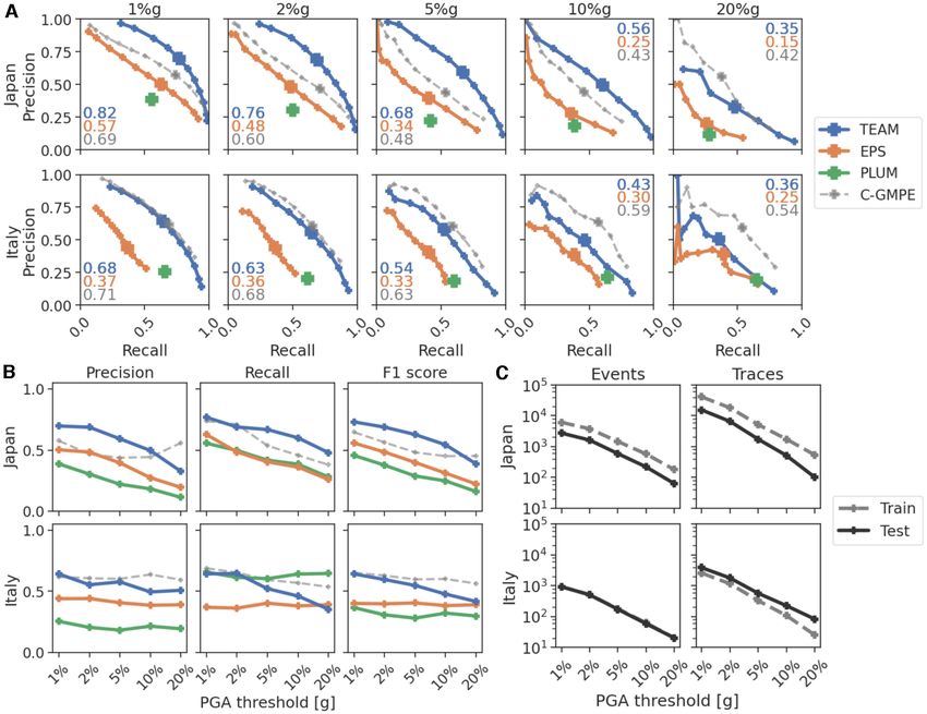
The transformer earthquake alerting model 647
Here, we present the transformer earthquake alerting model subdivided into three components: feature extraction, feature com-
(TEAM), a deep learning method for early warning, combining the bination, and density estimation (Fig. S1). Input to TEAM are
advantages of both classical early warning strategies while avoid- three, respectively six (three surface, three borehole), component
ing the deficiencies of prior deep learning approaches. We evaluate waveforms at 100 Hz sampling rate from multiple stations and the
TEAM on two data sets from regions with high seismic hazard, corresponding station coordinates. Furthermore, the model is pro-
namely Japan and Italy. Due to their complementary seismicity, this vided with a set of output locations, at which the PGA should be
allows to evaluate the capabilities of TEAM across scenarios. We predicted. These can be anywhere within the spatial domain of the
Downloaded from https://academic.oup.com/gji/article/225/1/646/6047414 by Bibliothek des Wissenschaftsparks Albert Einstein user on 16 February 2021
compare TEAM to two state-of-the-art warning methods, of which model and need not be identical with station locations in the training
one is prototypical for source based warning and one for propaga- set.
tion based warning. TEAM extracts features from input waveforms using a convo-
lutional neural network (CNN). The feature extraction is applied
separately to each station, but is identical for all stations. CNNs are
2 D ATA A N D M E T H O D S well established for feature extraction from seismic waveforms, as
they are able to recognize complex features independent of their
2.1 Data position in the trace. On the other hand, CNN based feature ex-
traction usually requires a fixed input length, inhibiting real-time
For our study we use two nation scale data sets from highly seis-
processing. We allow real-time processing through the alignment of
mically active regions with dense seismic networks, namely Japan
the waveforms and zero-padding: we align all input waveforms in
(13 512 events, years 1997–2018, Fig. 1) and Italy (7055 events,
time, that is, all start at the same time t0 and end at the same time t1 .
years 2008–2019, Fig. 2). Their seismicity is complementary, with
We define t0 to be 5 s before the first P-wave arrival at any station,
predominantly subduction plate interface or Wadati-Benioff zone
allowing the model to understand the noise characteristics. For t1
events for Japan, many of them offshore, and shallow, crustal events
we use the current time, that is, the amount of available waveforms.
for Italy. We split both data sets into training, development and test
We obtain constant length input, by padding all waveforms after
sets with ratios of 60:10:30. We employ an event-wise split, that
t1 with zeros up to a total length of 30 s. The feature extraction is
is, all records for a particular event will be assigned to the same
described in more detail in supplementary text S2.
subset. We do not explicitly split station-wise but due to temporary
TEAM combines the feature vectors and maps them to repre-
deployments there are a few stations in the test set which have no
sentations at the targets using a transformer (Vaswani et al. 2017).
records in the training set (Fig. 2). We use the training set for model
Transformers are attention-based neural networks for combining
training, the development set for model selection, and the test set
information from a flexible number of input vectors in a learnable
only for the final evaluation. We split the Japan data set chronologi-
way. To encode the location of the recording stations as well as of
cally, yielding the events between August 2013 and December 2018
the prediction targets, we use sinusoidal vector representations. For
as test set. For Italy, we test on all events in 2016, as these are of
input stations, we add these representations component-wise to the
particular interest, encompassing most of the central Italy sequence
feature vectors, for target stations we directly use them as inputs
with the Mw = 6.2 and Mw = 6.5 Norcia events (Dolce & Di Bucci
to the transformer. This architecture, processing a varying num-
2018). Especially the latter event is notably larger than any in the
ber of inputs, together with the explicitly encoded locations, allows
training set (Mw = 6.1 L’Aquila event in 2007), thereby challenging
TEAM to handle dynamically varying sets of stations and targets.
the extrapolation capabilities of TEAM.
The transformer returns one vector for each target representing pre-
Both data sets consist of strong motion waveforms. For Japan
dictions at this target. Details on the feature combinations can be
each station comprises two sensors, one at the surface and one
found in supplementary text S3.
borehole sensor, while for Italy only surface recordings are available.
From each of the vectors returned by the transformer, TEAM
As the instrument response in the frequency band of interest is flat,
calculates the PGA predictions at one target. Similar to the fea-
we do not restitute the waveforms, but only apply a gain correction.
ture extraction, the PGA prediction network is applied separately
This has the advantage that it can trivially be done in real-time. The
to each target, but is identical for all targets. TEAM uses mixture
data and pre-processing are further described in the supplement
density networks (Bishop 1994) returning Gaussian mixtures, to
text S1.
computes PGA densities. Gaussian mixtures allow TEAM to pre-
dict more complex distributions and better capture realistic uncer-
tainties than a point estimate or a single Gaussian. The full specifi-
2.2 TEAM
cations for the final PGA estimation are provided in supplementary
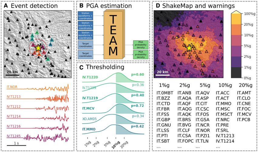
The early warning workflow with TEAM encompasses three sepa- text S4.
rate steps (Fig. 3): event detection, PGA estimation and threshold- TEAM is trained end-to-end using a negative log-likelihood loss.
ing. We do not further consider the event detection task here, as To increase the flexibility of TEAM and allow for real-time pro-
it forms the base of all methods discussed and affects them simi- cessing, we use training data augmentation. We randomly select
larly. The PGA estimation, resulting in PGA probability densities the stations used as inputs and targets in each training iteration. In
for a given set of target locations, is the heart of TEAM and de- addition, again in each training iteration, we randomly replace all
scribed in detail below. In the last step, thresholding, TEAM issues waveforms after a time t with zeros, matching the input representa-
warnings for each target locations where the predicted exceedance tion of real time data, to train TEAM for real-time application. These
probability p for fixed PGA thresholds surpasses a predefined data augmentations as well as the complete training procedure are
probability α. further described in supplementary text S5.
TEAM conducts end-to-end PGA estimation: its input are raw To mitigate the systematic underestimation of high PGA values
waveforms, its output predicted PGA probability densities. There observed in previous machine learning models, TEAM oversam-
are no intermediate representations in TEAM that warrant an im- ples large events and PGA targets close to the epicentre during
mediate geophysical interpretation. The PGA assessment can be training, which reduces the inherent bias in data towards smaller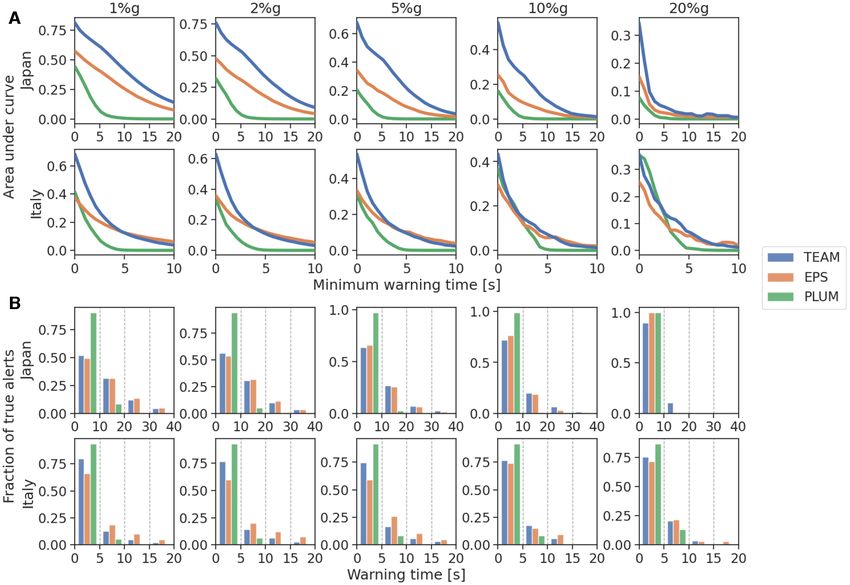
648       J. Münchmeyer et al.

                                                                                                                                                                      Downloaded from https://academic.oup.com/gji/article/225/1/646/6047414 by Bibliothek des Wissenschaftsparks Albert Einstein user on 16 February 2021
Figure 1. Map of the station (left-hand panel) and event (right-hand panel) distribution in the Japan data set. Stations are shown as black triangles, events as
dots. The event colour encodes the event magnitude. There are ∼20 additional events far offshore, which are outside the displayed map region in the catalogue.

Figure 2. Map of the station (left-hand panel) and event (right-hand panel) distribution in the Italy data set. Stations present in the training set are shown as
black triangles, while stations only present in the test set are shown as yellow triangles. Events are shown as dots with the colour encoding the event magnitude.
All events with magnitudes above 5.5 are shown as stars. The red stars indicate large training events, while the yellow stars indicate large test events. The inset
shows the central Italy region with intense seismicity and high station density in the test set. Moment magnitudes for the largest test events are given in the
inset.

PGAs. When learning from small catalogues or when applied to re-                        Our Italy data set is an example of this situation. Accordingly,
gions where events substantially larger than all training events can                 TEAM applies domain adaptation to this case: It first trains a joint
be expected, for example, because of known locked fault patches                      model using data from Japan and from Italy, which is then fine-
or historic records, TEAM additionally can use domain adapta-                        tuned using the Italy data on its own, except for the addition of
tion. To this end the training procedure is modified to include                      a few large, shallow, onshore events from Japan. We chose these
large events from other regions that are similar to the expected                     events, as for Italy one also expects large, shallow, crustal events
events in the target region. While records from those events will                    due to its tectonic setting and earthquake history. As we use events
differ in certain aspects, for example, site responses or the exact                  from Italy in both training steps and in particular in the second step
propagation patterns, other aspects, for example, the average ex-                    the overwhelming number of events are from Italy, we expect that
tent of strong shaking or the duration of events of a certain size,                  this scheme only results in a small degradation in the modelling of
will mostly be independent of the region in question. The domain                     the regional specifics of the Italy region.
adaptation aims to enable the model to transfer the region imma-
nent aspects of large events, at the cost of a certain blurring of
                                                                                     2.3 Baselines
the specific regional aspects of the target region. TEAM aims to
mitigate the blurring of regional aspects by the choice of training                  We compare TEAM to two state-of-the-art early warning methods,
procedure.                                                                           one using source estimation and one propagation based. As source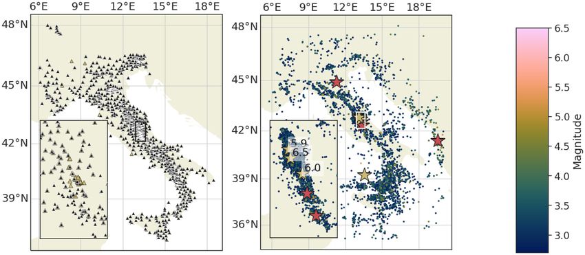
The transformer earthquake alerting model                    649

                                                                                                                                                                   Downloaded from https://academic.oup.com/gji/article/225/1/646/6047414 by Bibliothek des Wissenschaftsparks Albert Einstein user on 16 February 2021
Figure 3. Schematic view of TEAM’s early warning workflow for the October 2016 Norcia event (Mw = 6.5) 2.5 s after the first P-wave pick (∼3.5 s after
origin time). (a) An event is detected through triggering at multiple seismic stations. The waveform colours correspond to the stations highlighted with orange
to magenta outlines. The circles indicate the approximate current position of P (dashed) and S (solid) wave fronts. (b) TEAM’s input are raw waveforms and
station coordinates; it estimates probability densities for the PGA at a target set. A more detailed TEAM overview is given in Fig. S1. (c) The exceedance
probabilities for a fixed set of PGA thresholds are calculated based on the estimated PGA probability densities. If the probability exceeds a threshold α, a
warning is issued. The figure visualizes a 10 per cent g PGA level with α = 0.4, resulting in warnings for the stations highlighted. The colours correspond to
the stations with green outlines in (a). (d) The real-time shake map shows the highest PGA levels for which a warning is issued. Stations are coloured according
to their current warning level. The table lists all stations for which warnings have already been issued.

estimation based method we use the estimated point source ap-                      3 R E S U LT S
proach (EPS), which estimates magnitudes from peak displacement
during the P-wave onset (Kuyuk & Allen 2013) and then applies                      3.1 Alert performance
a GMPE (Cua & Heaton 2009) to predict the PGA. For simplicity,
                                                                                   We compare the alert performance of all methods for PGA thresh-
our implementation assumes knowledge of the final catalogue epi-
                                                                                   olds from light (1 per cent g) to very strong (20 per cent g) shaking,
centre, which is impossible in real-time, leading to overoptimistic
                                                                                   regarding precision, the fraction of alerts actually exceeding the
results for EPS. As propagation based method we chose an adap-
                                                                                   PGA threshold, and recall, the fraction of issued alerts among all
tation of PLUM (Kodera et al. 2018), which issues warnings if a
                                                                                   cases where the PGA threshold was exceeded (Meier 2017; Min-
station within a radius r of the target exceeds the level of shaking.
                                                                                   son et al. 2019). Precision and recall trade-off against each other
In contrast to the original PLUM, which operates on the Japanese
                                                                                   depending on α. While the PGA predictions of TEAM, EPS and
seismic intensity scale, IJMA (Shabestari & Yamazaki 2001), our
                                                                                   the C-GMPE are probabilistic, the thresholding transforms the pre-
adaptation applies the concept of PLUM to PGA, thereby making
                                                                                   dictions into alerts or non-alerts. The probability distribution de-
it comparable to the other approaches. Whereas IJMA is also a mea-
                                                                                   scribes the uncertainty of the models, for example, for the GMPE
sure of the strongest acceleration and is thus strongly correlated
                                                                                   the apparent aleatoric uncertainty from aspects not accounted for,
with PGA, it considers a narrower frequency band and imposes a
                                                                                   which makes false and missed alerts inevitable. The threshold value
minimum duration of strong shaking. As such, although the perfor-
                                                                                   controls the trade-off between both types of errors, and its ap-
mance might vary slightly for our PLUM-like approach compared
                                                                                   propriate value will depend on user needs, specifically the costs
to the original PLUM, it still exhibits its key features, in particular
                                                                                   associated with false and missed alerts. Therefore, to analyse the
the effects of the localized warning strategy. Additionally we apply
                                                                                   performance of the models across different user requirements, we
the GMPE used in EPS to catalogue location and magnitude as
                                                                                   look at the precision recall curves for different thresholds α. In
an approximate upper accuracy bound for point source algorithms
                                                                                   addition to precision and recall, we use two summary metrics: F1
(Catalogue-GMPE or C-GMPE). C-CMPE is a theoretical bound
                                                                                   score, the harmonic mean of precision and recall, and AUC, the
that can not be realized in real-time. It can be considered as an esti-
                                                                                   area under the precision recall curve. The evaluation metrics and
mate of the modeling error for point source approaches. A detailed
                                                                                   full setup of the evaluation are defined in detail in supplement
description of the baseline methods can be found in supplementary
                                                                                   text S7.
text S6.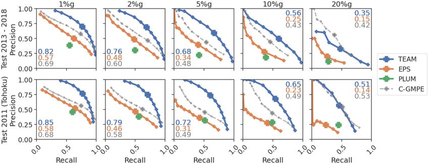
650       J. Münchmeyer et al.

                                                                                                                                                                   Downloaded from https://academic.oup.com/gji/article/225/1/646/6047414 by Bibliothek des Wissenschaftsparks Albert Einstein user on 16 February 2021
Figure 4. Warning statistics for the three early-warning models (TEAM, EPS, PLUM) for the Japan and Italy data sets. In addition, statistics are provided
for C-GMPE, which can only be evaluated post-event due to its reliance on catalogue magnitude and location. (a) Precision and recall curves across different
thresholds α = 0.05, 0.1, 0.2, . . . , 0.8, 0.9, 0.95. As the PLUM-like approach has no tuning parameter, its performance is shown as a point. Enlarged markers
show the configurations yielding the highest F1 scores. Numbers in the corner give the area under the precision recall curve (AUC), a standard measure
quantifying the predictive performance across thresholds. (b) Precision, recall and F1 score at different PGA thresholds using the F1 optimal value α. Threshold
probabilities α were chosen independently for each method and PGA threshold. (c) Number of events and traces exceeding each PGA threshold for training
and test set. Training set numbers include development events and show the numbers before oversampling is applied. For Italy training and test event curve are
overlapping due to similar numbers of events.

   TEAM outperforms both EPS and the PLUM-like approach for                        shortage of training data with high PGA values results in less well
both data sets and all PGA thresholds, indicated by the precision-                 constrained model parameters.
recall-curves of TEAM lying to the top-right of the baseline curves                    Using domain adaptation techniques, TEAM copes well with
(Fig. 4a). For any baseline method configuration, there is a TEAM                  the Italy data, even though the largest test event (Mw = 6.5) is
configuration surpassing it both in precision and in recall. Im-                   significantly larger than the largest training event (Mw = 6.1), and
provements are larger for Japan, but still substantial for Italy.                  three further test events have Mw ≥ 5.8. To assess the impact of this
To compare the performance at fixed α, we selected α values                        technique, we compared TEAM’s results to a model trained without
yielding the highest F1 score separately for each PGA thresh-                      it (Figs S2 and S3). While for low PGA thresholds differences are
old and method. Again, TEAM outperforms both baselines on                          small, at high PGA levels they grow to more than 20 points F1
both data sets, irrespective of the PGA level (Fig. 4b). Perfor-                   score. Interestingly, for large events, TEAM strongly outperforms
mance statistics in numerical form are available in Tables S1                      TEAM without domain adaptation even for low PGA thresholds.
and S2.                                                                            This shows that domain adaptation does not only allow the model to
   All methods degrade with increasing PGA levels, particularly                    predict higher PGA values, but also to accurately assess the region
for Japan. This degradation is intrinsic to early warning for high                 of lighter shaking for large events. Domain adaptation therefore
thresholds due to the very low prior probability of strong shaking                 helps TEAM to remain accurate even for events quite far from the
(Meier 2017; Minson et al. 2019; Meier et al. 2020). Furthermore,                  training distribution.
The transformer earthquake alerting model                   651

                                                                                                                                                                  Downloaded from https://academic.oup.com/gji/article/225/1/646/6047414 by Bibliothek des Wissenschaftsparks Albert Einstein user on 16 February 2021
Figure 5. Warning time statistics. (a) Area under the precision recall curve for different minimum warning times. All alerts with shorter warning times are
counted as false negatives. (b) Warning time histograms showing the distribution true alerts across distances for the different methods. Please note that the
total number of true alerts differs by method and is not shown in this subplot. Therefore the values of different methods cannot be directly compared, but only
the differences in the distributions. TEAM and EPS are shown at F1-optimal α, chosen separately for each threshold and method. Warning time dependence
on hypocentral distance is shown in Fig. S4.

3.2 Warning times                                                                     Warning times depend on α: a lower α value naturally leads to
                                                                                   longer warning times but also to more false positive warnings. At
In application scenarios, a user will usually require a certain warn-
                                                                                   F1-optimal thresholds α, EPS and TEAM have similar warning time
ing time, which is the time between issuing of the warning and
                                                                                   distributions (Fig. 5b, Table S3), but lowering α leads to stronger
first exceedance of the level of shaking, as this time is necessary
                                                                                   increases in warning times for TEAM. For instance, at 10 per cent g,
for taking action. As the previous evaluation considered prediction
                                                                                   lowering α from 0.5 to 0.2 increases average warning times of
accuracy irrespective of the warning time, we now compare the
                                                                                   TEAM by 2.3 s/1.2 s (Japan/Italy), but only by 1.1 s/0.1 s for EPS.
methods while imposing a certain minimum warning time. Actu-
                                                                                   Short times as measured here are critical in real applications: First,
ally, TEAM consistently outperforms both baselines across differ-
                                                                                   they reduce the time available for counter measures. Secondly, real
ent required warning times and irrespective of the PGA threshold
                                                                                   warning times will be shorter than reported here due to telemetry
(Fig. 5a). While the margin for TEAM compared to the baselines is
                                                                                   and compute delays. However, compute delays for TEAM are very
smaller for Italy than for Japan, TEAM shows consistently strong
                                                                                   mild: analysing the Norcia event (25 input stations, 246 target sites)
performance across different warning times. In contrast, EPS per-
                                                                                   for one time step took only 0.15 s on a standard workstation using
forms clearly worse at short warning times, the PLUM-based ap-
                                                                                   non-optimized code.
proach at longer warning times. The latter is inherent to the key
idea of PLUM and makes the method only competitive at high PGA
thresholds, where potential maximum warning times are naturally                    4 DISCUSSION
short due to the proximity between stations with strong shaking and
the epicentre (Minson et al. 2018). We further note that while the                 4.1 Calibration of probabilities
PLUM-like approach shows slightly higher AUC than TEAM for
short warning times at 20 per cent g, this is only a hypothetical re-              Even though TEAM and EPS give probabilistic predictions, it is
sult. As PLUM does not have a tuning parameter between precision                   not clear whether these predictions are well-calibrated, that is, if
and recall, this performance can actually only be realized for a spe-              the predicted confidence values actually correspond to observed
cific precision/recall threshold, where it performs slightly superior              probabilities. Calibrated probabilities are essential for threshold
to TEAM (Fig. 4a bottom right-hand panel).                                         selection, as they are required to balance expected costs of taking
652 J. Münchmeyer et al.
Downloaded from https://academic.oup.com/gji/article/225/1/646/6047414 by Bibliothek des Wissenschaftsparks Albert Einstein user on 16 February 2021
Figure 6. Scenario analysis of the 22 November 2016 MJ = 7.4 Fukushima earthquake, the largest test event located close to shore. Maps show the warning
levels for each method (top three rows) at different times (shown in the corner, t = 0 s corresponds to P arrival at closest station). Dots represent stations and
are coloured according to the PGA recorded during the full event, that is, the prediction target. The bottom row shows (left- to right-hand panels), the catalogue
based GMPE predictions, the warning time distributions, and the true positives (TP), false negatives (FN) and false positives (FP) for each method, both at a
2 per cent g PGA threshold. EPS and GMPE shake map predictions do not include station terms, but they are included for the bottom row histograms.
action versus expected costs of not taking action. We note that Italy, EPS is generally slightly overconfident, while TEAM is well
while good calibration is a necessary condition for a good model, calibrated, except for a certain overconfidence at 20 per cent g. We
it is not sufficient, as a model constantly predicting the marginal suspect that the worse calibration for the largest events is caused by
distribution of the labels would be always perfectly calibrated, yet the domain adaptation strategy, but the better performance in terms
not very useful. of accuracy clearly weighs out this downside of domain adaptation.
To assess the calibration, we use calibration diagrams (Figs S9
and S10) for Japan and Italy at different times after the first P
4.2 Insights into TEAM
arrival. These diagrams compare the predicted probabilities to the
actually observed fraction of occurrences. In general, both models We analyse differences between the methods using one example
are well calibrated, with a slightly better calibration for TEAM. event from each data set (Japan: Fig. 6, Italy: Fig. S5). All meth-
Calibration is generally better for Japan, where only EPS is slightly ods underestimate the shaking in the first seconds (left-hand column
underconfident at earlier times for the highest PGA thresholds. For Figs 6 and S5). However, TEAM is the quickest to detect the correctThe transformer earthquake alerting model 653
Downloaded from https://academic.oup.com/gji/article/225/1/646/6047414 by Bibliothek des Wissenschaftsparks Albert Einstein user on 16 February 2021
Figure 7. Precision recall curves for the Japanese data set using the chronological split (top panel) and using the events in 2011 as test set (bottom panel). The
year 2011 contains the Mw = 9.1 Tohoku event as well as its aftershocks.
extent of the shaking. Additionally, it estimates even fine-grained re- precision recall curves for the chronological split and the year 2011
gional shaking details in real-time (middle and right-hand columns). as test set. In general, the performance of all models stays similar
In contrast, shake maps for EPS remain overly simplified due to the when evaluated on the alternative split. A key difference between
assumptions inherent to GMPEs (right-hand column and bottom the curves is, that TEAM, in particular for high PGA thresholds,
left-hand panel). For the Japan example, even late predictions of does not reach similar levels of recall for 2011 as for the chrono-
EPS underestimate the shaking, due to an underestimation of the logical split, while achieving higher precision. As we will describe
magnitude. The PLUM-based approach produces very good PGA in the next paragraph, this trend probably results from a tendency
estimates, but exhibits the worst warning times. to underestimate true PGA amplitudes, which will naturally re-
Notably, TEAM predictions at later times correspond even bet- duce recall and boost precision. Nevertheless, the performance of
ter to the measured PGA than C-GMPE estimates, although these TEAM as quantified by the AUC actually improves, and signifi-
are based on the final magnitude (top right- and bottom left-hand cantly so for the highest thresholds. We suspect that this tendency
panels). For the Japan data, this is not only the case for the exam- for underestimation is either caused by the higher number of large
ple at hand, but also visible in Fig. 4, showing higher accuracy of events in the 2011 test set compared to the chronological split, or
TEAM’s prediction compared to C-GMPE for all thresholds except by the lower number of high PGA events in the training set without
20 per cent g on the full Japan data set. We assume TEAM’s supe- 2011.
rior performance is rooted in both global and local aspects. Global Fig. S6 presents a scenario analysis for the Tohoku event. All
aspects are the abilities to exploit variations in the waveforms, for models underestimate the event considerably, with the strongest
example, frequency content, to model complex event characteristics, underestimation for the EPS method. Even 20 s after the first
such as stress drop, radiation pattern or directivity, and to compare P wave arrival, all methods underestimate both the severity and
to events in the training set. Local aspects include understanding the extent of shaking. Due to its localized approach, the PLUM-
regional effects, for example, frequency dependent site responses, based model achieves the highest number of true warnings, albeit
and the ability to consider shaking at proximal stations. We note that at short warning times and a certain number of false positives,
for our Italy experiments, the modelling of local aspects resulting which due to the underestimation are totally absent from TEAM
from regional characteristics might be slightly degraded by the do- and EPS predictions. The performance of both EPS and TEAM is
main adaptation. However, the first-order propagation effects such likely degraded by the slow onset of the Tohoku event as described
as, for example, amplitude decay due to geometric spreading, are by Koketsu et al. (2011). According to Koketsu et al. (2011) the
similar between regions and therefore not negatively affected by the main subevent with a displacement of 36 m only initiated 20 s
domain adaptation. In conclusion, combining a global event view after the onset of the Tohoku event. Therefore only the first P
with propagation aspects, TEAM can be seen as a hybrid model waves for EPS or at most the first 25 s of waveforms for TEAM is
between source estimation and propagation. most likely insufficient to correctly estimate the size of the Tohoku
event.
For Italy, we showed that underestimation for large events can
be mitigated using transfer learning. However, the Tohoku event
4.3 TEAM performance on the Tohoku sequence
clearly shows the limitations of this strategy, as nearly no training
We evaluated TEAM for Japan on a chronological train/dev/test data for events of comparable size are available, even when using
split, as this split ensures the evaluation closest to the actual ap- events across the globe. Therefore, for the largest events alternative
plication scenario. On the other hand, this split put the M = 9.1 strategies need to be developed, for example, training using sim-
Tohoku event in March 2011 into the training set. To evaluate the ulated data. Furthermore, the 25 s of waveforms used by TEAM
performance for this very large event and its aftershocks, we trained in the current implementation may, for a very large event, not cap-
another TEAM instance using the year 2011 as test set and the re- ture the largest subevent. While we decided to use only 25 s of
mainder of the data for training and validation. Fig. 7 shows the event waveforms, as there is only insufficient training data of longer654 J. Münchmeyer et al.
events, this window could be extended when developing training Cochran, E.S., Bunn, J., Minson, S.E., Baltay, A.S., Kilb, D.L., Kodera, Y. &
strategies and models for the largest events. Hoshiba, M., 2019. Event detection performance of the plum earthquake
early warning algorithm in Southern California, Bull. seism. Soc. Am.,
109(4), 1524–1541.
Cua, G. & Heaton, T.H., 2009. Characterizing average properties of south-
5 C O N C LU S I O N ern California ground motion amplitudes and envelopes, EERL Report,
In this study we presented TEAM. TEAM outperforms existing Earthquake Engineering Research Laboratory, Pasadena, CA.
early warning methods in terms of both alert performance and Dipartimento di Fisica, Universitá degli studi di Napoli Federico, II, 2005.
Downloaded from https://academic.oup.com/gji/article/225/1/646/6047414 by Bibliothek des Wissenschaftsparks Albert Einstein user on 16 February 2021
Irpinia Seismic Network (ISNet), Istituto Nazionale di Geofisica e Vul-
warning time. Using a flexible machine learning model, TEAM
canologia (INGV).
is able to extract information about an event from raw wave- Dolce, M. & Di Bucci, D., 2018. The 2016–2017 central apennines seismic
forms and leverage the information to model the complex de- sequence: analogies and differences with recent Italian earthquakes, in
pendencies of ground motion. We point out two further aspects Recent Advances in Earthquake Engineering in Europe: 16th European
that make TEAM appealing to users. First, TEAM can adapt to Conference on Earthquake Engineering-Thessaloniki 2018, Geotechni-
various user requirements by combining two thresholds, one for cal, Geological and Earthquake Engineering, pp. 603–638, ed. Pitilakis,
shake level and one for the exceedance probability. As TEAM out- K., Springer International Publishing.
puts probability density functions over the PGA, these thresholds EMERSITO Working Group, 2018. Seismic network for site effect studies
can easily be adjusted by individual users on the fly, for exam- in Amatrice Area (Central Italy) (SESAA), Istituto Nazionale di Geofisica
ple, by setting sliders in an early warning system. Secondly, deep e Vulcanologia (INGV). https://doi.org/10.13127/SD/7TXeGdo5X8.
Geological Survey-Provincia Autonoma di Trento, 1981. Trentino seismic
learning models typically exhibit large performance improvements
network, International Federation of Digital Seismograph Networks,
from larger training data sets (Sun et al. 2017) due to the high 10.7914/SN/ST.
number of model parameters. In our study this reflects in the bet- Istituto Nazionale di Geofisica e Vulcanologia (INGV), 2008. INGV exper-
ter performance on the twofold larger Japan data set. This indi- iments network, Istituto Nazionale di Geofisica e Vulcanologia (INGV).
cates that TEAM’s performance can be improved just by collecting Istituto Nazionale di Geofisica e Vulcanologia (INGV), Istituto di Geologia
more comprehensive catalogues, which happens automatically over Ambientale e Geoingegneria (CNR-IGAG), Istituto per la Dinamica dei
time. Processi Ambientali (CNR-IDPA), Istituto di Metodologie per l’Analisi
Ambientale (CNR-IMAA), Agenzia Nazionale per le nuove tecnologie,
l’energia e lo sviluppo economico sostenibile (ENEA), 2018. Rete del
Centro di Microzonazione Sismica (CentroMZ), sequenza sismica del
AC K N OW L E D G E M E N T S 2016 in Italia Centrale, Istituto Nazionale di Geofisica e Vulcanologia
We thank the National Research Institute for Earth Science and (INGV), 10.13127/SD/ku7Xm12Yy9.
Disaster Resilience (NIED) for providing the catalogue and wave- Istituto Nazionale di Geofisica e Vulcanologia (INGV), Italy, 2006. Rete
sismica nazionale (RSN), Istituto Nazionale di Geofisica e Vulcanologia
form data for our Japan data set. We thank the Istituto Nazionale
(INGV), doi.org/10.13127/SD/X0FXnH7QfY.
di Geofisica e Vulcanologia and the Dipartimento della Protezione
Jozinović, D., Lomax, A., Štajduhar, I. & Michelini, A., 2020. Rapid
Civile for providing the catalogue and waveform data for our Italy prediction of earthquake ground shaking intensity using raw wave-
data set. JM acknowledges the support of the Helmholtz Einstein form data and a convolutional neural network, Geophys. J. Int., 222(2),
International Berlin Research School in Data Science (HEIBRiDS). 1379–1389.
We thank Matteo Picozzi for discussions on earthquake early warn- Karim, K.R. & Yamazaki, F., 2002. Correlation of JMA instrumental seismic
ing that helped improve the study design. We thank Hiroyuki Goto intensity with strong motion parameters, Earthq. Eng. Struct. Dyn., 31(5),
and an anonymous reviewer for their comments which helped to 1191–1212.
improve the manuscript. Kodera, Y., Yamada, Y., Hirano, K., Tamaribuchi, K., Adachi, S.,
The source code for TEAM and the baselines are available Hayashimoto, N., Morimoto, M., Nakamura, M. & Hoshiba, M., 2018.
The propagation of local undamped motion (PLUM) method: a simple
at https://github.com/yetinam/TEAM. The repository contains the
and robust seismic wavefield estimation approach for earthquake early
necessary instructions for downloading the Japan data set as well.
warning, Bull. seism. Soc. Am., 108(2), 983–1003.
The Italy data set was published as Münchmeyer et al. (2020). Koketsu, K., Yokota, Y., Nishimura, N., Yagi, Y., Miyazaki, S., Satake, K.,
Fujii, Y., Miyake, H., Sakai, S., Yamanaka, Y., et al., 2011. A unified
source model for the 2011 Tohoku earthquake, Earth planet. Sci. Lett.,
REFERENCES 310(3–4), 480–487.
Allen, R.M. & Melgar, D., 2019. Earthquake early warning: advances, sci- Kriegerowski, M., Petersen, G.M., Vasyura-Bathke, H. & Ohrnberger, M.,
entific challenges, and societal needs, Ann. Rev. Earth Planet. Sci., 47(1), 2019. A deep convolutional neural network for localization of clustered
361–388. earthquakes based on multistation full waveforms, Seismol. Res. Lett.,
Allen, R.M., Gasparini, P., Kamigaichi, O. & Bose, M., 2009. The status 90(2A), 510–516.
of earthquake early warning around the world: an introductory overview, Kuyuk, H.S. & Allen, R.M., 2013. A global approach to provide magnitude
Seismol. Res. Lett., 80(5), 682–693. estimates for earthquake early warning alerts, Geophys. Res. Lett., 40(24),
Belkin, M., Hsu, D., Ma, S. & Mandal, S., 2019. Reconciling modern 6329–6333.
machine-learning practice and the classical bias–variance trade-off, Proc. Lomax, A., Michelini, A. & Jozinović, D., 2019. An investigation of rapid
Natl. Acad. Sci., 116(32), 15 849–15 854. earthquake characterization using single-station waveforms and a convo-
Bishop, C.M., 1994. Mixture density networks, Tech. rep., Aston University. lutional neural network, Seismol. Res. Lett., 90(2A), 517–529.
Böse, M., Smith, D.E., Felizardo, C., Meier, M.-A., Heaton, T.H. & Clin- MedNet Project Partner Institutions, 1990. Mediterranean Very Broadband
ton, J.F., 2018. FinDer v.2: improved real-time ground-motion predictions Seismographic Network (MedNet), Mediterranean Very Broadband Seis-
for m2–M9 with seismic finite-source characterization, Geophys. J. Int., mographic Network (MedNet). Istituto Nazionale di Geofisica e Vul-
212(1), 725–742. canologia (INGV). https://doi.org/10.13127/SD/fBBBtDtd6q.
Chung, A.I., Henson, I. & Allen, R.M., 2019. Optimizing earthquake Meier, M.-A., 2017. How “good” are real-time ground motion predictions
early warning performance: ElarmS-3, Seismol. Res Lett., 90(2A), from earthquake early warning systems?, J. geophys. Res., 122(7), 5561–
727–743. 5577.The transformer earthquake alerting model 655
Meier, M.-A., Kodera, Y., Böse, M., Chung, A., Hoshiba, M., Cochran, E., S U P P O RT I N G I N F O R M AT I O N
Minson, S., Hauksson, E. & Heaton, T., 2020. How often can earthquake
early warning systems alert sites with high-intensity ground motion?, J. Supplementary data are available at GJ I online.
geophys. Res., 125(2), e2019JB017718, doi:10.1029/2019JB017718. Figure S1: Overview of the transformer earthquake alerting model,
Minson, S.E., Meier, M.-A., Baltay, A.S., Hanks, T.C. & Cochran, E.S.,
showing the input, the feature extraction, the feature combination,
2018. The limits of earthquake early warning: timeliness of ground motion
estimates, Sci. Adv., 4(3), eaaq0504.
the PGA estimation and the output. For simplicity, not all layers are
Minson, S.E., Baltay, A.S., Cochran, E.S., Hanks, T.C., Page, M.T., McBride, shown, but only their order and combination is visualized schemat-
Downloaded from https://academic.oup.com/gji/article/225/1/646/6047414 by Bibliothek des Wissenschaftsparks Albert Einstein user on 16 February 2021
S.K., Milner, K.R. & Meier, M.-A., 2019. The limits of earthquake early ically. For the exact number of layers and the size of each layer
warning accuracy and best alerting strategy, Sci. Rep., 9(1), 2478. please refer to tables S5 and S6. Please note that the number of
Mousavi, S.M. & Beroza, G.C., 2020. Bayesian-deep-learning estimation input stations and the number of targets are both variable, due to
of earthquake location from single-station observations, IEEE Transac- the self-attention mechanism in the feature combination. Ten in-
tions on Geoscience and Remote Sensing, IEEE, 58, 11, 8211–8224, stances of this network are trained independently and the results
10.1109/TGRS.2020.2988770. ensemble-averaged.
Mousavi, S.M. & Beroza, G.C., 2020. A machine-learning approach Figure S2: True positives (TP), false negatives (FN) and false posi-
for earthquake magnitude estimation, Geophys. Res. Lett., 47(1),
tives (FP) for the events in the Italy test sets causing the largest shak-
e2019GL085976, doi:10.1029/2019GL085976.
Münchmeyer, J., Bindi, D., Leser, U. & Tilmann, F., 2020. Fast earthquake
ing. The methods are the transformer earthquake alerting model
assessment and earthquake early warning dataset for Italy, GFZ Data without domain adaptation (TEAM base), the transformer earth-
Services, V 1.0., doi: 10.5880/GFZ.2.4.2020.004. quake alerting model (TEAM), the estimated point source algo-
Muthukumar, V., Vodrahalli, K., Subramanian, V. & Sahai, A., 2020. Harm- rithm (EPS) and PLUM-based approach. In addition, a GMPE with
less interpolation of noisy data in regression, IEEE J. Select. Areas Inform. full catalogue information is included for reference. Values α were
Theory, arXiv:1903.09139 [cs.LG] chosen separately for each threshold and method to yield the high-
National Research Institute For Earth Science And Disaster Resilience, est F1 score for the whole test set, but are kept constant across all
2019. Nied k-net, kik-net, National Research Institute for Earth Science events. TEAM with domain adaptation outperforms TEAM without
and Disaster Resilience, doi:10.17598/NIED.0004. domain adaptation consistently across all thresholds. This indicates
OGS (Istituto Nazionale Di Oceanografia E Di Geofisica Sperimentale),
that the domain adaptation not only allows TEAM to better predict
2016. North-East Italy Seismic Network. International Federation of Dig-
ital Seismograph Networks.OGS (Istituto Nazionale Di Oceanografia E
higher levels of shaking, but also to better assess large events in
Di Geofisica Sperimentale), https://doi.org/10.7914/SN/OX. general.
OGS (Istituto Nazionale di Oceanografia e di Geofisica Sperimen- Figure S3: Precision, recall and F1 score at different PGA
tale) and University of Trieste, 2002. North-East Italy Broadband thresholds for Italy including TEAM without domain adaptation.
Network. International Federation of Digital Seismograph Networks, Threshold values α were chosen independently for each method
https://doi.org/10.7914/SN/NI and PGA threshold to yield the highest F1 score. The meth-
Otake, R., Kurima, J., Goto, H. & Sawada, S., 2020. Deep learning model ods are the transformer earthquake alerting model without do-
for spatial interpolation of real-time seismic intensity, Seismol. Res. Lett., main adaptation (TEAM Base), the transformer earthquake alert-
91(6), 3433–3443. ing model (TEAM), the estimated point source (EPS) model and
Presidency of Counsil of Ministers - Civil Protection Department, 1972.
the PLUM-based model. In addition the graph shows the perfor-
Italian Strong Motion Network. Presidency of Counsil of Ministers -
Civil Protection Department, https://doi.org/10.7914/SN/IT.
mance of C-GMPE, a GMPE with full catalogue information for
RESIF - Réseau Sismologique et géodésique Français, 1995a. RESIF-RLBP reference.
French Broad-band network, RESIF-RAP strong motion network and Figure S4: Warning time and hypocentral distance between sta-
other seismic stations in metropolitan France, doi.org/10.15778/resif.fr. tion and event for each true alert at F1-optimal α. The white area
RESIF - Réseau Sismologique et géodésique Français, 1995b. Réseau corresponds roughly to the range of possible warning times and is
accélérométrique permanent (french accelerometrique network) (rap). bounded by the 90th percentile of the times between first detection
Shabestari, K.T. & Yamazaki, F., 2001. A proposal of instrumental seismic of an event (i.e. arrival of P wave at the closest station) and first
intensity scale compatible with mmi evaluated from three-component exceedance of the PGA threshold in recordings at that approximate
acceleration records, Earthq. Spectra, 17(4), 711–723. distance.
Snoek, J., et al., 2019. Can you trust your model’s uncertainty? evalu-
Figure S5: Scenario analysis of the 30 October 2016 Mw = 6.5
ating predictive uncertainty under dataset shift, in Advances in Neural
Information Processing Systems, 33rd Conference on Neural Information
Norcia earthquake, the largest event in the Italy test set. See Fig. 4
Processing Systems (NeurIPS 2019), Vancouver, Canada, pp. 13 969–13 in the main paper for further explanations. The bottom row diagrams
980. for this scenario analysis use a 10 per cent g PGA threshold.
Sun, C., Shrivastava, A., Singh, S. & Gupta, A., 2017. Revisiting unreason- Figure S6: Scenario analysis of the 11 March 2011 Mw = 9.1
able effectiveness of data in deep learning era, in Proceedings of the IEEE Tohoku earthquake, the largest event in the Japan data set. See
International Conference on Computer Vision, pp. 843–852. Fig. 4 in the main paper for further explanations. The bottom
Universita della Basilicata, 2005. UniBAS, Italian National Institute of Geo- row diagrams for this scenario analysis use a 2 per cent g PGA
physics and Volcanology (INGV). threshold.
University of Genova, 1967. Regional seismic network of north western Italy. Figure S7: Training and validation loss curves for the Japan TEAM
international federation of digital seismograph networks, International
model and the fine-tuning step of the Italy TEAM model. Each
Federation of Digital Seismograph Networks, 10.7914/SN/GU.
Vaswani, A., Shazeer, N., Parmar, N., Uszkoreit, J., Jones, L., Gomez, A.N.,
line shows the loss curve for one ensemble member with colours
Kaiser, Ł. & Polosukhin, I., 2017. Attention is all you need, in Advances matching between training and validation curves. The models used
in Neural Information Processing Systems, pp. 5998–6008. are determined by the minimum validation loss and are denoted by
Wald, D.J., Quitoriano, V., Heaton, T.H. & Kanamori, H., 1999. Relationships black crosses. The models were evaluated after the training epoch
between peak ground acceleration, peak ground velocity, and modified indicated on the x-axis, that is, the leftmost point of each curve
Mercalli intensity in California, Earthq. Spectra, 15(3), 557–564. already includes one epoch of training.656 J. Münchmeyer et al.
Figure S8: Predictions and residuals of the GMPEs derived in this exceeding a threshold if at least one station exceeded this threshold
study. All PGA values are given as log units using m s–2 . Every point during the event. The number of exceedances in the test set for
refers to one recording. Solid lines indicate running means, dashed Italy is disproportionally high compared to the number of events
lines denote the running standard deviation around the running in the test set. This is caused by the high seismic activity and the
mean. Orange crosses denote mean and standard deviations for higher station density in 2016. Traces for Japan always refer to six
magnitude ranges with insufficient data to infer a continuous line. component traces, while for Italy it refers to three component traces.
Window sizes are 0.24 m.u./10 km (Italy) and 0.44 m.u./53 km Table S5: Architecture of the feature extraction network. The input
Downloaded from https://academic.oup.com/gji/article/225/1/646/6047414 by Bibliothek des Wissenschaftsparks Albert Einstein user on 16 February 2021
(Japan). Overall σ is 0.29 for Italy and 0.33 for Japan. The plotted dimensions of the waveform data are (time, channels). FC denotes
magnitude values have been offset by random values between –0.05 fully connected layers. As FC layers can be regarded as 0D convolu-
and 0.05 m.u. for increased visibility. tions, we write the output dimensionality in the filters column. The
Figure S9: Calibration diagrams for Japan at different times after ‘Concatenate scale’ layer concatenates the log of the peak ampli-
the first P detection and different PGA thresholds. The confidence tude to the output of the convolutions. Depending on the existence
is defined as the probability of exceeding the PGA threshold as pre- of borehole data the number of input filters for the first Conv1D
dicted by the model. Each bar represents the traces with a confidence layer is 64 instead of 32 in the non-borehole case.
value inside the limits of the bar. Its height is given by the accuracy, Table S6: Architecture of the transformer network. Please note that
the fraction of traces actually exceeding the threshold among all even though the transformer in TEAM does not apply dropout,
traces in the bar. For a perfectly calibrated model, the confidence we explicitly state this in the table, as transformers commonly use
equals the accuracy. This is indicated by the dashed line. We note dropout.
that accuracy estimations for the high PGA thresholds are strongly
Please note: Oxford University Press is not responsible for the con-
impacted by stochasticity due to the small number of samples.
tent or functionality of any supporting materials supplied by the
Figure S10: Calibration diagrams for Italy at different times after
authors. Any queries (other than missing material) should be di-
the first P detection and different PGA thresholds. For a further
rected to the corresponding author for the paper.
description see the caption of figure S9.
Table S1: Performance statistics for Japan. Probability thresholds
α were chosen to maximize F1 scores and are shown in the last
A P P E N D I X : D ATA S O U R C E S
column. The AUC value does not depend on the threshold α. PGA
indicates the used PGA threshold. We obtained our Japan catalogue and waveforms from NIED and
Table S2: Performance statistics for Italy. Probability thresholds the NIED KiK-net (National Research Institute For Earth Science
α were chosen to maximize F1 scores and are shown in the last And Disaster Resilience 2019). For our Italy data set we use the
column. The AUC value does not depend on the threshold α. PGA INGV catalogue and waveforms from the 3A (Istituto Nazionale
indicates the used PGA threshold. di Geofisica e Vulcanologia (INGV) 2018), BA (Universita della
Table S3: Relative warning times of the algorithms in seconds. Basilicata 2005), FR (RESIF - Réseau Sismologique et géodésique
Positive values indicate longer average warning times for the second Français 1995a), GU (University of Genova 1967), IT (Presidency
method, negative values shorter warning times. The difference in of Counsil of Ministers - Civil Protection Department 1972), IV
average warning times is calculated from all event station pairs, (Istituto Nazionale di Geofisica e Vulcanologia (INGV) 2006), IX
where both methods issued correct warnings. No value is reported (Dipartimento di Fisica, Universitá degli studi di Napoli Federico
if this set is empty. We set α for TEAM and EPS to the optimal II 2005), MN (MedNet Project Partner Institutions 1990), NI (OGS
value in terms of F1 score. (Istituto Nazionale di Oceanografia e di Geofisica Sperimentale)
Table S4: Data set statistics for the full data set and the test set. The 2002), OX (OGS (Istituto Nazionale di Oceanografia e di Ge-
lower boundary of the magnitude category is the 5th percentile of ofisica Sperimentale) 2016), RA (RESIF - Réseau Sismologique
the magnitude; this limit is chosen as each data set contains a small et géodésique Français 1995b), ST (Geological Survey-Provincia
number of unrepresentative very small events. The upper boundary Autonoma di Trento 1981), TV (Istituto Nazionale di Geofisica e
is the maximum magnitude. The lower part of the table shows how Vulcanologia (INGV) 2008) and XO (EMERSITO Working Group
often each PGA threshold was exceeded. An event is counted as 2018) networks.You can also read