Consumption changes due to expected future income as a result of Covid-19

Consumption changes due to expected future
 income as a result of Covid-19
 Matilda Keskinen Melissa Au
 guskeskima@student.gu.se gusaumet@student.gu.se

 Abstract
 This thesis aims to investigate the effects of the pandemic on individuals’
 expectations regarding future income and thus their consumption behavior. The
 research will therefore contribute with new insights into the relationship between
 consumer behaviour and income expectations, which can be useful for future
 studies and for policy design during this or future pandemics.

 To analyse the consumption changes due to expected future income as a result of
 the pandemic, a web survey was sent to the mailing list of the School of Business,
 Economics and Law at the University of Gothenburg. Consequently, the sample
 mainly consists of Swedish students at a mean age of 25 years old. The data was
 later used in various ordered probit regressions to analyse the variables of interest.
 The results have shown that an employee’s expected future income is not only
 dependent on how their income has been affected as a result of Covid-19, but also
 if they are at risk of losing their job. When testing what economic factors affect a
 student expected future income, none of the included variables were significant,
 which can be due to the sample not being adequately sized. It was also found that
 change in consumption is generally associated with expected future income.

 In conclusion, the analysis has given us an important insight on how Covid-19 has
 affected future income expectations and thereby consumption. This can be
 beneficial when predicting the effects future pandemics, hence introducing more
 suited policies that can reduce the negative effect on the economy.

Keywords: consumer behaviour, expected future income, COVID-19, pandemic, crisis

Bachelor´s thesis in Economics, 15 credits
Spring Semester 2021
Supervisor: Oben K. Bayrak

Department of Economics
School of Business, Economics and Law
University of Gothenburg

Acknowledgements

It is with great joy and pride that we finally submit our bachelor’s thesis in Economics. The
process has at times been stressful and intense, but at the same time full of anticipation and
elation over what the next chapter will bring.

Firstly, we would like to thank our supervisor Oben K. Bayrak, who has guided us through
this process, listened to our ideas, and provided us with helpful insights. Secondly, we would
like to thank our family and friends who have supported and believed in us. Lastly, we would
like to thank the 365 respondents who answered our survey, and hence made this thesis
possible.

And to you who are reading this, we hope you will have an enjoyable read.

 Melissa Au & Matilda Keskinen
 2021-06-07

 2

TABLE OF CONTENTS
1 INTRODUCTION ....................................................................................................................................... 4
 1.1 BACKGROUND ........................................................................................................................................... 4

 1.2 OUR CONTRIBUTION .................................................................................................................................. 5

2 LITERATURE REVIEW AND THEORETICAL FRAMEWORK ...................................................... 6
 2.1 LITERATURE REVIEW ................................................................................................................................. 6

 2.2 THEORETICAL FRAMEWORK ...................................................................................................................... 8

3 DATA AND METHODOLOGY .............................................................................................................. 14
 3.1 SURVEY DESCRIPTION.............................................................................................................................. 14

 3.2 VARIABLES .............................................................................................................................................. 16

 3.3 CONCERNS ............................................................................................................................................... 20

 3.4 LIMITATIONS ........................................................................................................................................... 21

4 RESULTS ................................................................................................................................................... 23
 4.1 SPEARMAN’S RANK CORRELATION TEST ................................................................................................. 26

 4.2 REGRESSIONS .......................................................................................................................................... 27

5 DISCUSSION ............................................................................................................................................. 35
6 CONCLUSIONS ........................................................................................................................................ 38
7 REFERENCES .......................................................................................................................................... 39
APPENDIXES ..................................................................................................................................................... 44
 APPENDIX A: ILLUSTRATIONS OF VARIABLES ................................................................................................... 44

 APPENDIX B: HYPOTHETICAL CHOICE EXPERIMENT (QUANTITATIVE RISK PREFERENCE) ................................. 50

 APPENDIX C: HYPOTHETICAL CHOICE EXPERIMENT (QUANTITATIVE TIME PREFERENCE) ................................. 51

 APPENDIX D: SURVEY QUESTIONS AND ANSWERS ............................................................................................. 52

 APPENDIX E: STATA OUTPUT ............................................................................................................................ 52

 3

1 Introduction
1.1 Background

After 118 000 confirmed cases in 114 countries and approximately 5000 lives lost, the World
Health Organization (hereafter WHO) finally declared Covid-19, a new variant of
Coronavirus, as a pandemic on March the 11th 2020. In order to control the spread of the
virus, nearly 100 countries enforced either partial or full lockdowns by the end of March 2020
(BBC, 2020, 7th April). Both at a global and national level, economies have affected adversely
due to lockdowns, travel restrictions, and restrictions on businesses in order to slow down the
spread of Covid-19.

One example of such an adverse effect was observed shortly after WHO declaring Covid-19
as a pandemic: Dow Jones tumbled by 10% on March 12th, 2020, breaking the record high
one day drop since 1987 (Stevens, Fitzgerald & Imbert, 2020). Furthermore, the OMX
Stockholm 30 dropped by 10.26% from March 11th to March 12th, 2020 (Avanza, n.d.).
Despite the developments of new vaccines, it looks like the effects will not disappear soon:
For example, the Swedish Public Employment Service (2020) predicts that the unemployment
rate will reach its all-time high at 11.4% during 2021, also breaking the record high
unemployment rate since the third millennium. Furthermore, according to the statistics
provided by UC (n.d.), bankruptcies in Sweden increased by 19% between January-April
2019 and January-April 2020.

Besides the macroeconomic effect, there is also an emerging literature investigating the
microeconomic side of the issue, particularly focusing on consumer behaviour. This thesis
aims to investigate the effects of the pandemic on individuals through the relationship
between their expectations regarding future income and their consumption behaviour. These
expectations will then form the basis for a behavioural economic analysis of how
consumption today has been affected due to uncertainty in future income, especially during
the uncertainty provided by a pandemic. The analysis is based on data collected from a web
survey, conducted between the 21st of April 2021 and the 29th of April 2021.

The remaining parts of the thesis are structured as follows: Section 2 explains the theories
which will be the base of analysis and relevant previous research. Section 3 provides the

 4

details about the web survey and the variables used in the analysis, alongside the concerns and
limitations of the methodology. Section 4 presents the results by first exploring the
relationship between variables, particularly using correlations and proceed with the
regressions addressing the research questions. Section 5 provides a discussion of the results
and theories included in this study. Lastly, Section 6 concludes the thesis.

1.2 Our contribution

The purpose of this thesis is to analyse the effects of the pandemic on individuals’
expectations regarding future income, and thereby their consumption behaviour. In particular,
the following research questions will form the base of the study:

 1. What economic factors during a pandemic affects an individual’s expected future
 income?
 2. Does the expectation of future income affect consumption today?

Our research will therefore contribute with new insights into the relationship between
consumer behaviour and income expectations, and serve as a benchmark if similar studies are
conducted later during this or future pandemics. Moreover, understanding and predicting the
behaviours of an individual coherently lies at the core of designing effective public policies
(Camerer and Loewenstein, 2003). The objective of this study is to contribute to the design of
policies during the pandemic by exploring the relationship between future income
expectations and consumption.

As the unemployment rate is predicted to reach a level of 11.4% in Sweden (The Swedish
Public Employment Service, 2020), a plausible hypothesis is thus that a concern will arise
amongst individuals since they are afraid of losing their current employment. As a reaction, it
is expected that the individuals, in the short term, will decrease their consumption and
increase their savings (since the future income is expected to fall) according to Fisher’s two-
period consumption model, explained in detail in Section 2.1.1.

The thesis will contribute to the field with its emphasis on the relationship between
expectations of future income, and consumption today.

 5

2 Literature review and theoretical framework
Since the outbreak, a considerable amount of research papers has been published,
investigating how Covid-19 has affected consumer behaviour. However, to date, research
exploring the relationship between consumer behaviour and income expectations during the
pandemic seems to be lacking. To provide a deeper understanding of the field, excerpts from
previous research, relevant to this thesis, will be presented below. In general, a majority of the
literature show that the economic uncertainty caused by Covid-19 has led to a change in
consumption behaviour, mainly a decrease in consumption. Some literature also points out
that this consumption change might be permanent.

2.1 Literature review

According to Kohli et al. (2020), Covid-19 has started a permanent shift in consumer
behaviour: through digital acceleration, shifts in consumer preferences, and economic
downturn, caused by the pandemic, both the individual consumer and the companies will get
the opportunity to shape “the Next Normal”. Furthermore, a consequence of the pandemic is
the increase in self-isolation, which has limited the individual’s movement outside of their
homes. Digitalization has therefore been essential as an adaption to the pandemic, for instance
making remote working and learning more common. The report further explains that self-
isolation, in addition to economic uncertainty, has resulted in this behavioural change in the
consumers. An increase in online purchases, and preference for trusted brands, as well as
reduced shopping frequency, but increased basket size, are some of the consumer changes
according to the study. For these changes are to remain permanent, the satisfaction of the
individuals with their new experiences will play a significant role, as the authors continue to
state changes in behaviour as non-linear. Hence, the next normal will emerge when the
society and economy have recovered to the pre-pandemic level, and the consumers are no
longer constrained by the Covid-19 restrictions.

Christelis et al. (2020) investigate the relationship between the drop in household spending
and the household’s concern regarding the financial consequences caused by Covid-19. The
study is based on new panel data collected through a monthly survey of representative
households, during the first wave of the pandemic. The households of interest were located in
the six largest economics in the euro area, namely Germany, France, Italy, Spain,

 6

Netherlands, and Belgium. The study found that financial concerns due to Covid-19 have led
to a significant decrease in the individuals’ willingness to consume, particularly in non-
durable goods. Despite the findings being significant, it is not surprising as it is in accordance
with models of precautionary savings and liquid constraints. Further, the consumption
decrease is explained not to be induced by health concerns due to the pandemic, but rather the
concern that Covid-19 will have unexpected future consequences on the economy. It is also
shown that the younger, the unemployed, and those with liquidity constraint expresses a
greater financial concern than the rest of the population. Thus, the researchers believe that by
supporting these vulnerable groups with targeted government interventions, the drop in
consumption will not be as immense.

An important conclusion is provided by Loxton et al. (2020) who state that the Covid-19
pandemic has generated a similar response in consumer behaviour as previous historic crises,
such as the SARS outbreak in 2002-04, Hurricane Irma in 2007, and the Christchurch
earthquake in 2011. To reach this conclusion, an extensive literature review was performed,
as well as an analysis of consumer spending data on primarily the American and Australian
market. The study showed that the Covid-19 pandemic has led to consumers exhibiting both
panic buying and herd mentality behaviours, which has been exploited by firms seeing it as a
business opportunity. Moreover, in line with Maslow’s Hierarchy of Needs Model, the
researchers found that consumer purchasing behaviour adapts to prioritize necessities in times
of crisis. Media was also found to be of great importance in influencing consumer behaviour
during Covid-19, increasing the effects of the previously mentioned behaviours. As the study
was published in June 2020, still at an early stage on the pandemic, it aims to add value and
act as a benchmark to future long-term studies of Covid-19.

The paper by van Bavel et al. (2020) explains the importance of social and behavioural
science to successfully manage the pandemic. The researchers highlight the value of
understanding human behaviour, for instance, threat perception, stress, and coping. This in
order for epidemiologists and policymakers to align the general public with the
recommendations for controlling the spread of the infection. The discussion was based on
circumstances that may align with the Covid-19 pandemic, such as hypothetical scenarios
conducted in a laboratory setting. This because at the time of publication (May 2020) there
was still a lack of research on the social scientific consequences of Covid-19, according to the

 7

paper. Similarly to the previously mentioned study, the Economics Observatory (2020)
investigates how, to limit the pandemic, individuals must change their behaviour. For this to
be possible, the researchers recommend the policymakers to take behavioural economics,
such as cognitive biases, pro-social behaviour, and feelings of civil duty, into consideration
when designing the guidelines for Covid-19. Their discussion is based on pre-existing
behavioural economic research and theories.

To control for the pandemic, many countries worldwide have enforced a lockdown. While the
lockdown may have reduced the spread of the disease, it has led to major economic
consequences. Cobion et al. (2020) focus on the economic consequences of a lockdown using
data from surveys conducted on a representative sample of U.S. households, between January
2020 and April 2020. The researchers observed how the timing of lockdowns affected the
households’ consumer behaviour and macroeconomic expectations differently, with the result
that counties with an early lockdown express a more pessimistic outlook towards the future.
For example, the households report an expectation of a substantially higher unemployment
rate and lower future inflation. The increased uncertainty towards the future has also led the
household to reallocate their assets into safer options, such as selling stocks in exchange for
liquid forms of savings. Furthermore, households have reduced their consumption and
increased their saving as a form of precaution. To conclude, the researchers highlight the
immense cost of a lockdown, with the intention that policymakers should keep the
repercussions of a lockdown in mind before implementing it.

2.2 Theoretical framework

This section will contain theoretical models that will later support and broaden the discussion.
The theories included in this section will be the two-period consumption model, time
preference, risk preference, ambiguity attitude, and Maslow’s Hierarchy of Needs Model.

2.2.1 The two-period consumption model

To analyse consumer behaviour, the two-period consumption model will serve as an
explanatory theory of how a rational individual makes consumptions choices. This relates to

 8

the uncertainty caused by Covid-19, since if an individual expects to lose their current
income, they will compensate by reducing their consumption today to increase their savings.
The increased amount of savings will enable the individual to consume more in the future
(despite their income level), thereby smoothing out the consumption over the two periods.

The two-period consumption model was developed by the economist Fisher (1930), which
allows analysing how rational individuals make intertemporal consumption choices. The
model considers a consumer who lives for two periods, present and future. For the model to
be plausible, Fisher made a few crucial assumptions: One of the most fundamental
assumptions is that consumers gain utility only from intertemporal consumption. He suggests
that individuals consider both the present (period one) and the future (period two) when
deciding how much to consume and save. Income, investments, and assets are the only
instruments to achieve the individual's goal – to maximize consumption which is constraint by
their income. Furthermore, as a simplification, he assumes that the consumer will not have
any assets after period two. We now proceed with explaining the elements of the model
starting with the intertemporal budget constraint, followed by the intertemporal utility
function.

The intertemporal budget constraint. At the beginning of period one, the consumer has no
assets. The consumer then earns income 1 and consumes 1 in period one. In period two, she
earns 2 and consumes 2 . Furthermore, the consumer has the option to either borrow (if 1 is
greater than 1 ) or save her income (if 1 is greater than 1 ). If she earns an income that is
greater than what she consumes in period one, she will save money, thus resulting in a
positive asset in period two, 2 . As a result, she will earn (1 + ) 2 due to the real interest
rate. If she on the other hand consumes more than her income in period one, then she will
borrow money, causing a negative 2 and pay back (1 + ) 2 . As further simplifications, the
model assumes that the consumer is a price-taker and takes at its given level, without trying
to influence the real interest rate (Gottfries, 2013).

Thus, the consumer faces two budget constraints, one in period one, and one in period two.
 1 + 2 = 1 (1)
 2 = 2 + (1 + ) 2 (2)

 9

By combining the budget constraints for both periods, the so-called “lifetime budget
constraint” is derived, which suggests that the discounted values of consumption have to be
equal to the discounted values of income.
 2 2 
 1 + = 1 + (3)
 1+ 1+ 

The intertemporal utility function. For the model to be feasible, Gottfries (2013) mentions
the following assumption. That is, individuals gain utility by consumption, therefore,
 ′ ( ) > 0. However, consumption will eventually run into a diminishing return, i.e. that
consumption will increase utility level by a smaller amount for each unit of increase in
consumption, hence, ′′ ( ) < 0. Furthermore, it is expected that individuals put less weight
on future utility compared to the present. Given that the consumer lives in two periods, the
lifetime utility ( 1 , 2 ) depends on the distribution of consumption in period one and period
two. Thus, giving us the following lifetime utility function:
 ( 2 )
 ( 1 , 2 ) = ( 1 ) + (4)
 1+ 

where ( ) denotes the consumer’s utility given at the consumption level in period and 
represents the discount factor implying how the individual values consumption today
compared to consumption in the future. The parameter takes values between zero and one: 
moves towards one when a consumer places a large value on present utility, thus being more
impatient. Considering the assumption that individuals put less weight on future utility
compared to the present, will never be less than zero.

Maximizing utility subject to the budget constraint. The two-period consumption model
assumes that consumers’ main goal is to maximize utility, which is achieved by consumption.
Hence, the marginal rate of substitution (MRS) has to be equal to the relative price of
consuming today and consuming in the future.
 ′ ( 1 ) ′( 1 ) 1 + (5)
 ′
 = 1+ → ′ =
 ( 2 ) / (1 + ) ( 2 ) 1 + 

Given that the real interest rate is equal to the individual’s discount rate, the utility gain due to
consumption in period one must equal to the utility in period two. This condition can only be
achieved if the consumption level in period one is equal to the consumption in period two. In

 10

conclusion, an individual will always choose to smooth out her consumption when possible
(Gottfries, 2013).

2.2.2 Time preference

Time preference is one of the main factors describing an individual’s discount rate in the two-
period consumption theory devolved by Fisher (1930). Thus, it is highly relevant for the
analysis. Intuitively, time preference can be defined as how people value future cash flows
compared to present cash flows. Therefore, time preference will reflect a person’s level of
savings and level of consumption.

An individual’s time preference is mainly reliant on her characteristics, which can fluctuate
depending on the individual’s life stage and different circumstances. Fisher (1930) argues that
children are more impatient as they lack foresight and self-control, however with time, their
level of patience will change depending on different factors. Namely, when the children enter
adulthood and have a family, their patience will increase as raising an offspring requires
foresight.

Furthermore, an individuals’ time preference will vary depending on their income. Fisher
suggests that a person with low income will be more impatient, thus spending more today as
saving for the future might not be possible. In addition, uncertainty is a significant factor that
may affect an individual’s time preference as Fisher argues that a person who is uncertain of
life will be more impatient as saving for the vague future might not increase utility. The
theory of time preference developed by Fisher is further strengthened by Jetter et al. (2020) as
they suggest that a man’s time preference has been more sensitive after the global economic
crisis of 2008.

2.2.3 Risk preference

In order to make rational consumption choices today, an individual will base their decisions
on future outcomes (Dimmock et al., 2013), for instance, expected future income. Thus, risk
preference plays an important role in analysing the effect of the pandemic on individuals’
expectations regarding future income. This can be exemplified by an individual, who as a

 11

result of Covid-19 has an unstable income source. Given that the individual is risk-seeking, it
is plausible to assume that they will keep their consumption level and savings persistent,
making them more vulnerable to a possible negative income shock. Whereas a risk avert
individual will choose to decrease their consumption today in order to increase their savings,
making them more prepared for an income loss.

Dohmen et al. (2011) state that an individual’s risk attitude is primarily innate, thus often kept
on a rather constant level. McLeod (2020) further suggests that risk preference is a product of
innate drives, the environment an individual is raised in, and how they were nurtured. Risk
attitude is, however, not time-invariant as individuals’ risk preference will have minor
fluctuations depending on different circumstances (Dohmen et al. 2011). This statement is
further supported by Vionea and Filip (2011) as they suggest that economic crises may cause
consumers to be more sensitive to risk, thus avoiding long-term decisions. Similarly,
Andersen et al. (2019) claim that a financial crisis will result in reduced risk-taking in the
future. Whether individuals’ decision-making is influenced by their risk preference
consciously or unconsciously, it is an important factor in understanding consumer behaviour.

2.2.4 Ambiguity attitude

To make informed decisions regarding future outcomes, for example, expected future income,
both ambiguity and risk should be taken into account (Dimmock et al., 2013). Consequently,
the thesis chose to analyse ambiguity as a complement to risk preferences. According to
Dimmock et al. (2013), ambiguity refers to your decision making under unknown
probabilities, while risk refers to your decision making under known probabilities. An
ambiguity averse individual is in economic literature described as preferring the known over
the unknown (behavioraleconomics.com, n.d.). Further, relevant research has been conducted
by Osaki and Schlesinger (2014) examining the effect of ambiguous shocks on future income
in a two-period consumption-saving model.

 12

2.2.5 Maslow’s Hierarchy of Needs Model

The American psychologist Abraham Maslow developed in 1943 the model Maslow’s
Hierarchy of Needs, which has over the years become a well-publicized motivational theory
in psychology. The model is often portrayed as a five-tiered pyramid, with each level of the
pyramid representing human needs in a hierarchical division. The bottom first and second
level represents the basic needs, consisting of physiological and safety needs. Continuing
upwards, the third and fourth level represents the psychological needs, consisting of self-
esteem and belonging. At the top is the fifth level representing the self-fulfilment needs,
consisting of self-actualization. The purpose of the hierarchical division is that to reach the
higher levels of self-fulfilment needs, the lower-level needs must first be satisfied. A
statement that has been criticised, both by other researchers (Kaur, 2013; McLeod, 2007) and
Maslow himself (Maslow, 1987). Regardless of the criticism, the model will in this thesis act
as an inspirational tool to distinguish between “wants” and “needs” within human behaviour.

In line with Maslow’s Hierarchy of Needs Model, Loxton et al. (2020) have found that
consumer purchasing behaviour adapts to prioritize necessities in times of crisis, such as the
Covid-19 pandemic. Thus, the model is highly relevant for this thesis as it is aimed to study
how individuals change their consumption of different types of goods during crises.

 13

3 Data and methodology
The following section will provide a description of the web survey and a brief description of
the sample’s demographics. It will then proceed with an in-depth explanation of the variables
used in the analysis, alongside with the concerns and limitations of the methodology.

3.1 Survey description

To collect the data needed for our analysis, an anonymous web survey was conducted. The
survey was published on social media platforms and sent to the mailing list of the School of
Business, Economics and Law at the University of Gothenburg (with 4532 respondents), on
the 21st of April 2021, and on the 22nd of April 2021, respectively.

When designing the survey, it was kept in mind that the participants would mainly be students
between 20-30 years old living in Gothenburg and the surrounding area. Thus, in
consideration of possible language barriers, both among exchange students and those who are
not as comfortable with Swedish, the survey was provided in both English and Swedish.
Equally important was to encourage the respondents to answer truthfully. A problem with
self-reported questions in a survey is the risk of response bias, which occurs when
respondents want to portray themselves in line with social norms (Furnham, 1986).
Consequently, the survey was conducted anonymously.

Before the survey was sent to the sample, a pilot survey was conducted on family and friends
(N=10) to gain feedback which would help to clarify and improve the survey. The pilot
survey resulted in minor grammatical changes and reformulation of ambiguous questions
which could be misunderstood by the sample.

To increase the participation rate, the respondents were offered to partake in a lottery with the
chance to win 200kr, which was informed in the introduction part of the survey. According to
related literature, the promise of an incentive creates a significant increase in participation,
compared to a situation where no potential reward is offered (Singer et al., 1999). Further, a
potential prize of 200kr is a cost-effective way for a study of this smaller size to create an
incentive, rather than to offer a reward to all participants. To further increase the participation
rate by minimizing non-responses, it was aimed to have as many closed-end questions as
possible. This method also facilitates the survey for the respondents.

 14

For the Swedish version of the survey, a total of 344 responses were collected, while the
English survey only had 21 respondents. To identify the characteristics of the sample, the
respondents were at first asked a few sociodemographic questions, such as their gender, age,
main occupation, etc.

On average, the survey took seven minutes to complete. To improve the quality of the data
later used for the analysis’ regression, respondents who completed the survey under four
minutes or over one hour were manually removed from the dataset. Consequently, 14
respondents out of 365 were withdrawn from the dataset, leaving us with 225 women, 125
men and 1 non-binary respondent. With approximately 62% female respondents, there is a
risk of gender bias. However, it is not expected for the analysis to suffer from gender bias, as
women, in general, are more likely to participate in online surveys (Smith, 2008). As a result
of mainly sharing the questionnaire on social media and the University of Gothenburg’s
mailing list, the mean age of the survey’s respondents were 25 years old (median = 24 years
old).

Table 1: Demographics of the sample

After obtaining the sociodemographic characteristics, the questionnaire proceeds with
questions eliciting expectations regarding employment and income. Those with an
employment were for example asked about the probability of them losing their job due to
Covid-19, as well as the pandemic affecting their income negatively on a 5-point Likert
scale.1

1
 The Likert scale is leading method in the field of behavioural science, used to measure human behaviour. The
5-point scale was applied due to its advantage of being able to be statistically tested in a regression model (Joshi
et al, 2015).

 15

Whereas the students were asked which degree they are studying, and to estimate the
probability of them not getting a job after their degree. To analyse if this estimate is correlated
with the consequences of the pandemic, the students were also requested to state when they
expect to graduate. According to Statistics Sweden, hereafter SCB, the national employment
rate decreased by 2.0% from February 2020 to June 2020 (SCB, 2021a) as a result of Covid-
19. Thus, it is arguable that the pandemic has had a significant impact on the labour market. It
is, therefore, assumable that a student who finishes their degree within one year is more
negatively affected by the pandemic than a student who finishes in four years.

The respondents who neither work nor study were asked to state unemployed as their main
occupation. Subsequently, the unemployed respondents were asked if they have been
dismissed from a previous job due to Covid-19. This is relevant for the analysis of expected
future income since we assume that if an induvial has lost a previous source of income, they
will have changed their current consumption behaviour as a result. It is also expected that the
unemployed, due to the negative impact on income, will consume less than the other
occupations. To analyse the unemployed respondent’s attitude towards the labour market, it
was asked whether they have actively searched for a job during their time as an unemployed.
It is open to discussion that an individual who has actively searched for a job for a longer
period without succeeding might have a more negative view on expected future income.

3.2 Variables
3.2.1 Dependent variables

Expected future income. A significant assumption made in the analysis is that an
individual’s perception of the future, in particular their expectation of future income, might
vary depending on their current occupation. Given that an individual work in a line of
business that has been negatively affected by Covid-19, such as restaurants, it is plausible for
them to lose their job. As a result, they will have a more negative expected future income. To
analyse the variable of interest, i.e. expectation of future income, respondents were asked to
specify their level of agreement or disagreement on a few questions based on their
occupation. By combining the data obtained, an aggregated variable representing expected
future income was developed.

 16

As a student, the subject was asked to estimate the likelihood of not finding a job after their
degree, thus generating the variable nojobstud. To analyse if this concern is due to Covid-19,
they were also asked when they expect to finish their degree. The variable nojobstud was then
weighted to capture the uncertainty caused by Covid-19. The students who predict to finish
their degree within a year were given more weight, thus assigned the highest level of
uncertainty. Contrary, the students with a longer time left to graduation were assigned less
weight to their answer, resulting in the final value of the variable probnojob:

 = ( 

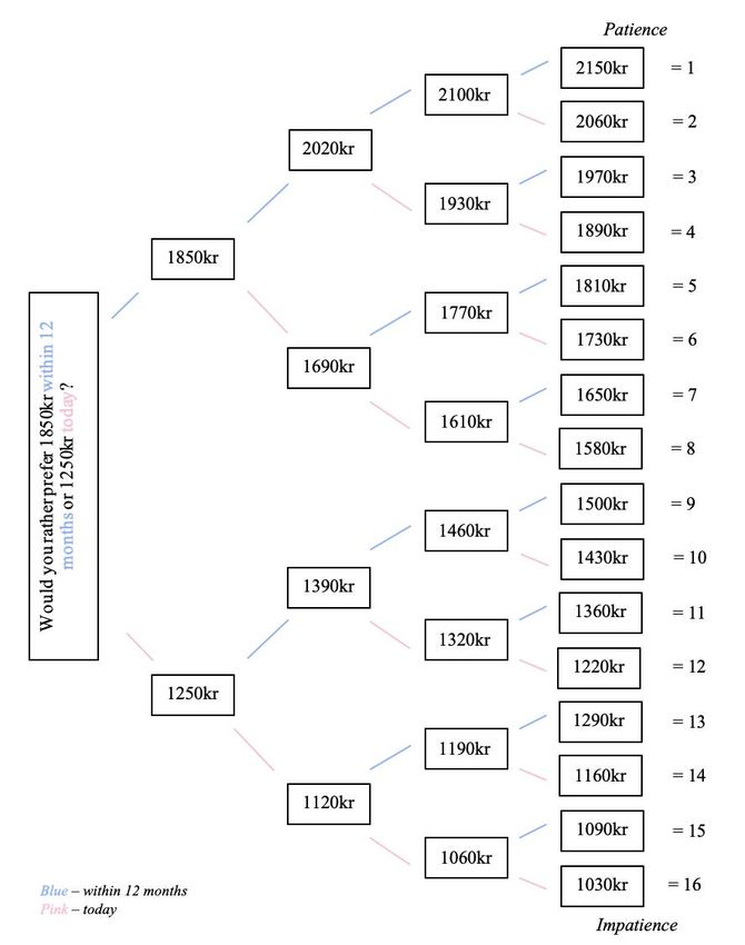
market entails. For this reason, the students with an employment were asked to estimate the
likelihood of their income to be negatively affected due to Covid-19. Unlike the respondents
who only study, their answers were not weighted since the uncertainty due to Covid-19 is
already captured in the question. The respondents who have a full-time or part-time job were
asked the same question, thus generating the variable neginc.

Unemployed was the last occupation alternative, where the respondents were asked to
estimate the likelihood of them not getting a job due to Covid-19. The estimate of the
respondents was then used to analyse their expectation on future income, resulting in the
variable nojobunemp.

Consumption behaviour. To measure how individuals have changed their consumption due
to Covid-19, they were given four different baskets of goods. The respondents were then
asked to state whether their expenditure in the corresponding basket has increased or
decreased on a 5-point Likert scale. These baskets were divided into necessities, inexpensive
durable goods, expensive durable goods, and leisure activities. To clarify for the participants,
a description of each basket was provided. It is not reasonable for each individual in the
sample to be fully aware of their spending habits in different baskets of good. With
consideration to this, a few proxy questions were included to avoid response bias. According
to the intertemporal budget constraint developed by Fisher (1930), savings are expected to
increase given a decrease in consumption, and vice versa. Therefore, the proxy questions
asked the participants whether their savings and investments had increased or decreased
during the same period.

3.2.2 Independent variables

Time preference. To evaluate how the respondents value present and future income flows, a
hypothetical experiment was conducted. The experiment consisted of four scenarios, which
enable the subject to choose between a payment “today”, and a larger payment “in 12
months”, based on the paper written by Falk et al. (2016). Depending on which alternative
was selected, the follow-up questions were altered. Similarly, to the previously mentioned
hypothetical scenario measuring risk preference, this experiment followed the structure of the
staircase method (Cornsweet, 1962). The respondent’s time preference was assigned a

 18

number from 1 to 16 to correspond to each respondent’s time discount rate when compiling
the data.2

Risk preference. By providing the participants with four hypothetical scenarios, it was
possible to measure their risk preference based on the staircase method (Cornsweet, 1962).
They were asked to choose between a guaranteed payment of 1600kr or a lottery with an
equal chance to receive 4800kr and 0kr. The respondents were then assigned three follow up
question in alignment with their initial choice. In each follow-up question, the guaranteed
payment and the lottery payment was modified based on their previous answer. When
compiling the data, the participants are assigned a number from 1 to 16, in order to evaluate
their attitude towards risk.3

Ambiguity. The survey measured ambiguity attitude in a set of two hypothetical questions,
inspired by the urn experiment conducted by Ellsberg (1961) and the supporting paper by
Dimmock et al. (2013). At first, the participants were asked to choose between two boxes
containing 100 balls each. The ambiguous box had an unknown distribution of purple and
orange balls, while the unambiguous box had a known distribution of 50 purple and 50 orange
balls. For the participant to win in the hypothetical scenario, they have to draw a purple ball.
The respondents were therefore asked to choose either the ambiguous box or unambiguous
box to draw the ball from. The selected box indicates the subject to be either ambiguity averse
or ambiguity seeking, respectively. The respondents could also choose the alternative to be
indifferent towards the boxes, indicating them to be ambiguity neutral. Later, the subject was
presented with a matching probability experiment, to measure their level of ambiguity and to
control for the previous question. The experiment provided the participant with an ambiguous
box, containing an unknown distribution of 100 balls, and an empty box. The level of
ambiguity was then measured by giving the participant the opportunity to choose the number
of winning/purple balls, which would make them indifferent between the two boxes.

Line of business. The respondents who are employed, both students with an employment and
full-time/part-time employees, were asked to state their line of business. This to analyse if

2
 Visual explanation in Appendix C.
3
 Visual explanation in Appendix B.

 19

certain businesses have been more affected by the economic consequences caused by Covid-
19. It is also interesting to analyse whether line of business is a relevant variable when
examining change in consumption and expectations on future income. However, due to the
smaller sample size, no statistical significance was achieved as the survey only conducted a
few respondents for each line of business. The decision was thus taken to categorise the
business based on Covid-19’s impact on labour demand. Thereby generating the dummy
variable safebus which take the value 1 if respondents work in a field where Covid-19 has had
a small or no impact on labour demand. For respondents who work in a line of business where
Covid-19 has had a large negative effect on labour demand, the dummy variable riskbus was
created. The respondents whose line of business is not specified are placed in the variable
othbus. To support vulnerable businesses that have had financial difficulties as a result of
Covid-19, the Swedish government is discussing to reintroduce the policy from 2020 where
companies can receive a rent subsidy issued by the state (Regeringskansliet, 2021a). These
businesses, according to the Swedish government are classified as financially vulnerable
(Regeringskansliet, 2021b). Hence the classification made by the Swedish government
formed the basis for the categorization in the variables safebus and riskbus.

3.3 Concerns

To analyse the data collected from the survey it is intended to run an ordered probit
regression. Thus, it is utterly important for the sample to be randomized, to avoid correlation
between the error term and variables of interest. Randomization eliminates selection bias,
giving us the true causal effect. As mentioned above, the web survey was primarily shared
through the researchers’ social media platforms and sent to the students at the School of
Business, Economics and Law at the University of Gothenburg. Consequently, a majority of
the respondent were students from the University of Gothenburg and the researchers’
acquaintances. It is, therefore, presumable that the respondents share specific characteristics,
hence, the variables in the ordered probit regression can be biased. Considering that the
survey is non-mandatory, the respondents are predominantly self-selected. It is also arguable
that the response rate is higher for people who are more affected alternatively more interested
in consumer behaviour/Covid-19, resulting in further selection bias. To control for this issue,
the survey contained a few questions aiming to identify the demographics and characteristics

 20

of the respondents. To further control for randomization, the sample was clustered. By
assigning each respondent a unique number, clustering was made achievable, giving us a
more accurate true casual effect.

To measure the respondent’s preference in ambiguity, risk and the present compared to the
future, they were given a variety of hypothetical questions, causing the analysis to be
vulnerable to hypothetical bias. However, in a study by Falk et al. (2016) the hypothetical
questions are found to have the same explanatory ability as incentivized choice experiments.
Furthermore, we have a few self-reported questions that can cause response bias, as
respondents either do not know the truthful answer or want to portray themselves with
socially desirable traits (Furnham, 1986).

In line with the objective of this study to investigate the true effect Covid-19 has had on
expected future income and thereby consumption, the respondents were asked to state if and
how their consumption has changed during the pandemic. As it is conceivable that other
unobservable factors may have an impact on the participant’s consumption during Covid-19,
the regression we intend to perform may suffer from endogeneity problems.

Moreover, it will be difficult to infer the findings to Sweden as a county since the survey is
mainly shared in Gothenburg and the surrounding area. Fact is that different regions are
affected differently by Covid-19 (EY, 2020), therefore, the survey sample is not
representative on a national level. Lastly, given that the sample is not adequately sized, it is
hard to obtain a statistically significant result that can be inferred.

Due to the concerns and eventual biases in this section, it is not plausible to make strong
inferences made about the population. Therefore, as a result of limited resources and time, the
purpose of this analysis is not to give significant results, but rather to give an insight on how
expectations of future income have been affected by uncertainty as a result of Covid-19.

3.4 Limitations

To facilitate the survey, it was aimed to keep the questionnaire as short as possible, only
containing relevant questions. Hence, it was not feasible to include all possible effects that
may have an impact on expectations on future income. For instance, the effect of health

 21

concern due to Covid-19 that may affect expected future income is not included as its
independent variable. Given that an individual expects to be severely ill due to the pandemic,
it is presumable for them to adapt their spending habits as income is expected to decrease, as a
result of not being able to work. Therefore, health concern due to Covid-19 is captured in the
independent variables included in the regression model. This argument is supported by the
paper written by Christelis et al. (2020), since the researchers found that health concerns do
not have a statistically significant impact on consumption, as an independent variable.

As mentioned under section 3.3, the ordered probit regression that we plan to regress may
suffer from endogeneity problems. These endogeneity problems can be avoided if more
survey questions were included, consequently, giving the regression model more control
variables. The trade-off of including more questions is however making the survey more
difficult and time-consuming for the respondents. Therefore, in consideration of the paper
written by Vicente & Reis (2010) and their recommendation of keeping surveys rather short
to receive more engaged respondents and to minimize the drop-out rate, additional questions
were not included.

 22

4 Results

The following section will start with a description of variables relevant to the study, along
with statistic measures. It will then proceed with a Spearman’s Rank Correlation test for the
variables of interest, as the data obtained from the survey mainly consists of ordinal data from
Likert scales. This to investigate if the regressions suffer from multicollinearity problems.

At last, the research questions will be analysed with ordered probit regressions due to the
ordinal data mentioned above. This method has also been done on related analyses which are
based on ordinal data (Müller & Rau, 2021).

Table 2: Descriptive statistics of variables

 Variable Description Mean Median Std.dev. Max Min

 woman =1 if the respondent is a woman 0.6429 1 0.4798 1 0

 age the respondent’s age 25.5727 24 7.0666 65 15

 par =1 if the respondent lives with a 0.1937 0 0.3958 1 0

 parent(s)

 partn =1 if the respondent lives with a partner 0.4074 0 0.4921 1 0

 alone =1 if the respondent lives alone 0.3447 0 0.4760 1 0

 stud =1 if the respondent is a student 0.6154 1 0.4871 1 0

 emp =1 if the respondent has an employment 0.3789 0 0.4858 1 0

 of any type

 bach =1 if the respondent studies a bachelor’s 0.6290 1 0.4838 1 0

 degree

 mast =1 if the respondent studies a master’s 0.3194 0 0.4670 1 0

 degree

 higsch =1 if the respondent is in high school 0.0097 0 0.0981 1 0

 probnojob the likelihood of the respondent not 1.9231 1.6 1.1352 5 0.4

 getting a job after their degree due to
 Covid-19

 emptype =1 if the respondent has a permanent 0.5940 1 0.4929 1 0

 employment contract

 23

safebus =1 if the respondent works in a line of 0.4812 0 0.5015 1 0

 business where Covid-19 has a little to no
 impact on labour demand

 riskbus =1 if the respondent works in a line of 0.1504 0 0.3588 1 0

 business where Covid-19 has a large
 impact on labour demand

disbeen =1 if the respondent has been dismissed 0.0963 0 0.2961 1 0

 from a previous job due to Covid-19

dismight the likelihood of the respondent losing 1.3609 1 0.8379 5 1

 their job due to Covid-19

 neginc the likelihood of the respondent’s income 1.8195 1 1.1732 5 1

 being affected negatively due to Covid-19

 incint1 =1 if the respondent has an average 0.4586 0 0.5002 1 0

 monthly income of 0kr – 15 000kr

 incint2 =1 if the respondent has an average 0.2556 0 0.4379 1 0

 monthly income of 15 001kr – 25 000kr

 incint3 =1 if the respondent has an average 0.1729 0 0.3796 1 0

 monthly income of 25 000kr – 40 000kr

 incint4 =1 if the respondent has an average 0.1128 0 0.3175 1 0

 monthly income of 40 001kr or more

 avinc Covid-19’s impact on the respondent’s 2.8718 3 0.8771 5 1

 average income

 chgnec change in consumption of necessities 3.1966 3 0.8236 5 1

 chgchd change in consumption of inexpensive 2.7009 3 1.0248 5 1

 durable goods

 chgexd change in consumption of expensive 2.7635 3 0.9818 5 1

 durable goods

 chglei change in consumption of leisure goods 2.7550 3 1.2432 5 1

 chgcon total change in consumption 2.8540 3 0.6463 5 1

 chgsav change in average savings 3.4644 3 1.0681 5 1

 chginv change in average investments 3.5641 3 1.0000 5 1

 24

globec =1 if the respondent will spend more 0.2194 0 0.4144 1 0

 today given that the global economy will
 get better

 savings =1 if the respondent has savings 0.9402 1 0.2375 1 0

 sav1 =1 if the respondent’s savings can 0.1303 0 0.3371 1 0

 support their living for 1-3 months

 sav2 =1 if the respondent’s savings can 0.2000 0 0.4006 1 0

 support their living for 3-6 months

 sav3 =1 if the respondent’s savings can 0.6697 1 0.4710 1 0

 support their living for 6 months or more

 timep quantitative time preference 9.0484 8 6.3320 16 1

 risk quantitative risk preference 6.0969 5 3.5875 16 1

 ambave =1 the if the respondent is ambiguity 0.5670 1 0.4962 1 0

 avert

 ambseek =1 the if respondent is ambiguity seeking 0.1368 0 0.3340 1 0

 ambneu =1 if the respondent is ambiguity neutral 0.2962 0 0.4572 1 0

 amb matching probability question measuring 0.0797 0 0.2797 0.5 -0.49

 the respondent’s level of ambiguity

Illustrations of the variables are presented in Appendix A. From the statistic measures, such as
the mean and the median, the overall consumption remains unchanged during Covid-19.
Furthermore, the variable neginc has a median of 1 indicating that a majority of the
respondents with an employment report a low likelihood of their average monthly income
being negatively affected due to Covid-19. The students also report a low likelihood of not
getting an employment after their degree due to Covid-19.

 25

4.1 Spearman’s Rank Correlation test

In order to examine the correlation for the independent variables, a Spearman’s Rank
Correlation test is conducted. Only the correlations that are found interesting and significant
are mentioned below.4 For the correlation test, a significance level of 10% is specified.

Table 3: Spearman correlation test for the whole sample
 woman age timep risk
 woman 1.0000
 age -0.1037 1.0000
 timep -0.0602 -0.1037 1.0000
 risk -0.1449 -0.0861 -0.0594 1.0000

By conducting the correlation test for the whole sample, woman and risk attitude shows a
significant correlation at -0.1449 (p=0.0107), indicating that women are more risk-averse in
comparison to men. This relationship is consistent with the findings from Falk et al. (2018).
Additionally, it is found that time preference and age have a positive correlation at 0.1027
(p=0.0548), implying a positive relationship between impatience and age. This finding is also
in line with Fisher’s (1930) theory about time preference.

Table 4: Spearman correlation test for the students
 avinc chgcon chgsav bach probnojob
 avinc 1.0000
 chgcon 0.1975 1.0000
 chgsav 0.1733 -0.1110 1.0000
 bach 0.0808 0.0834 0.0198 1.0000
 probnojob -0.0822 -0.0936 -0.0890 -0.1150 1.0000

For the 216 students in the sample, a significant positive relationship is found between
average income and change in total consumption (Spearman’s =0.1975, p=0.0036). Thus, an
individual with an increased average income will report an overall increased consumption.
Average income and change in savings have a correlation coefficient of 0.1733 (p=0.0107),
suggesting that an increase in average income will increase savings and vice versa. These
findings are rational, as an individual will change their level of savings and/or consumption

4
 The correlation coefficient will be discussed; however, the interpretations do not imply a causal effect. Due to
limited resources, the analysis will not cover the causal effects between the variables.

 26

given a change in average disposable income. Furthermore, it is found that the variables bach
and probnojob are negatively correlated, with a correlation coefficient of -0.1150 (p=0.0919).
Hence, given that a respondent is studying for a bachelor’s degree, then they will report a
lower probability of not receiving a job after their degree due to Covid-19.

Table 5: Spearman correlation test for the respondent with an employment
 dismight emptype avinc chgcon chgsav neginc
 dismight 1.0000
 emptype -0.1577 1.0000
 avinc -0.4281 0.0706 1.0000
 chgcon -0.0018 -0.0304 0.1853 1.0000
 chgsav -0.1952 -0.0816 0.3464 0.0898 1.0000
 neginc 0.5809 -0.1102 -0.5343 -0.0272 -0.2502 1.0000

When analyzing the correlation for the employed (n=133), a negative correlation of -0.01577
(p=0.0699) is found for the variables dismight and emptype. This, indicating that an employee
with a permanent employment is less likely to state a high probability of losing their current
job. Similar to the students, a significant positive correlation was found both between average
income, change in total consumption (Spearman’s =0.1880, p=0.0309) and change in
savings (Spearman’s =0.3487, p=0.0000). Furthermore, a negative correlation of -0.2660
(p=0.0021) is reported for neginc and chgsav, i.e. that the more likely Covid-19 is to affect
the respondent’s income negatively, the more likely it is for them to decrease their savings.

4.2 Regressions

In order to study the research questions presented in Section 1.2, namely the relationship
between expectation on future income and consumption behaviour during a pandemic,
different regressions are performed. Since the dependent variable in the models consists of
ordinal data from Likert scales, it is decided to run an ordered probit regression. The ordered
probit regression is an appropriate method as it is used in previous analyses with similar data
(Müller & Rau, 2021). To control for the regressions, sociodemographic variables are
included in all models, for example, woman, age, and id. The variable id is manually
generated, where each respondent is assigned a unique number, which is used to cluster the
standard errors in the regressions, and thereby reduce the possibility of non-random sampling.
The regressions are also run with robust standard errors, however, only the clustered standard

 27

errors are presented in table 6 and 7 as no significant difference was discovered between the
two standard errors. The results from the robust standard errors can be found in the output
from Stata.

4.2.1 What economic factors during a pandemic affects an individual’s expected
 future income?

In the following two regressions, we will test for the first research question stated in the title
of the section, divided into employees and students. To avoid endogeneity problems, control
variables were included in both regressions. This along with the variable avinc captures
Covid-19’s impact on the respondent’s average income.

Employees. In addition to the control variables and avinc, variables for employment type and
line of business were included. To capture the individual’s expectation of being dismissed
from their current employment due to the pandemic, dismight is used as an explanatory
variable. If a person expects to lose their employment, it is plausible that their expectation of
future income will be negatively affected as well. It is also arguable that if an individual has
been dismissed from a previous job due to Covid-19, then the individual will be more mindful
of the consequences the pandemic has on the labour market. Thus, the variable disbeen will
affect the outcome variable, expectation of future income.

 = 1 ( ) + 2 ( ) + 3 ( ) + 4 ( ) + 5 ( ) + 6 ( )
 + 7 ( ) + 8 ( ) + 9 ( ) + 10 ( )
 + 11 ( ℎ ) + 12 ( ) + ℰ ( 1 )

For regression 1 ( 1 ) with n=132, two significant variables were obtained, dismight and
avinc at a significance level at =0.05. The coefficient for dismight is positive, indicating that
if the respondent has a high likelihood of losing their employment, then it will increase the
probability of the respondent stating a negative expectation of future income due to Covid-19.
For avinc, the regression reports a negative coefficient. Implying that if a respondent’s
average monthly income has increased due to the pandemic, then it is less likely for the
subject to report a negative expectation of future income due to Covid-19.

 28