Globalization in the Time of - COVID-19 8184 2020

8184
 2020
 Original Version: March 2020
 This Version: May 2020

Globalization in the Time of
COVID-19
Alessandro Sforza, Marina Steininger

Impressum:

CESifo Working Papers
ISSN 2364-1428 (electronic version)
Publisher and distributor: Munich Society for the Promotion of Economic Research - CESifo
GmbH
The international platform of Ludwigs-Maximilians University’s Center for Economic Studies
and the ifo Institute
Poschingerstr. 5, 81679 Munich, Germany
Telephone +49 (0)89 2180-2740, Telefax +49 (0)89 2180-17845, email office@cesifo.de
Editor: Clemens Fuest
https://www.cesifo.org/en/wp
An electronic version of the paper may be downloaded
· from the SSRN website: www.SSRN.com
· from the RePEc website: www.RePEc.org
· from the CESifo website: https://www.cesifo.org/en/wp

CESifo Working Paper No. 8184

 Globalization in the Time of COVID-19

 Abstract

The economic effects of a pandemic crucially depend on the extent to which countries are
connected in global production networks. In this paper we incorporate production barriers
induced by COVID-19 shock into a Ricardian model with sectoral linkages, trade in
intermediate goods and sectoral heterogeneity in production. We use the model to quantify the
welfare effect of the disruption in production that started in China and quickly spread across the
world. We find that the COVID-19 shock has a considerable impact on most economies in the
world, especially when a share of the labor force is quarantined. Moreover, we show that global
production linkages have a clear role in magnifying the effect of the production shock. Finally,
we show that the economic effects of the COVID-19 shock are heterogeneous across sectors,
regions and countries, depending on the geographic distribution of industries in each region and
country and their degree of integration in the global production network.
JEL-Codes: F100, F110, F140, F600.
Keywords: COVID-19 shock, globalization, production barrier, sectoral interrelations,
computational general equilibrium.

 Alessandro Sforza Marina Steininger
 University of Bologna Ifo Institute – Leibniz Institute for
 piazza Scaravilli Economic Research at the University of
 Bologna / Italy Munich / Germany
 alessandro.sforza3@unibo.it steininger@ifo.de

For an updated version click here:
https://drive.google.com/open?id=1SeHWV20aIWdqpdwZSiVfm57BJrUqKy6Q

This version: April 20, 2020, first version: April 1, 2020
We thank Lorenzo Caliendo, Lisandra Flach, Annalisa Loviglio, Luca David Opromolla,
Gianmarco Ottaviano, Fernando Parro, Vincenzo Scrutinio, Tommaso Sonno for useful
discussion. We thank Matilde Bombardini for sharing the Chinese Census data with us. All
errors are ours.

1 Introduction

Globalization allows firms to source intermediate inputs and sell final goods in many different
countries. The diffusion of a local shock through input-output linkages and global value
chains has been extensively studied (see for example Carvalho et al. (2016)) but little is
known on how a pandemic affects global production along with its diffusion.1
In this paper we study the role of global production linkages in the transmission of a pandemic
shock across countries. We exploit an unprecedented disruption in production in the recent
world history, namely the global spread of COVID-19 virus disease, to instruct a multi-
country, multi-sector Ricardian model with interactions across tradable and non-tradable
sectors observed in the input-output tables. We use the model to quantify the trade and
welfare effects of a disruption in production that started in China and then quickly spread
across the world. The spread of COVID-19 disease provides a unique set-up to understand
and study the diffusion of a global production shock along the global value chains for three
main reasons. First, it is possibly the biggest production disruption in the recent world
history. With around 2.424.419 cases, 166.256 deaths and millions of people in quarantine
around the world to date2 , the spread of COVID-19 disease is the largest pandemic ever
experienced in the globalized world.3 Second, the COVID-19 shock is not an economic shock
in its nature, hence its origin and diffusion is independent from the fundamentals of the
economy. Third, differently from any other non-economic shock experienced before, it is
a global shock. Indeed, while the majority of natural disasters or epidemics have a local
dimension, the spread of the COVID-19 disease has been confined to the Chinese province
of Hubei only for a few weeks, to then spread across the entire world.
Understanding the effects of a global production disruption induced by a pandemic is com-
plex. We build on the work by Caliendo and Parro (2015) who develop a tractable and simple
model that allows to decompose and quantify the role that intermediate goods and sectoral
linkages have in amplifying or reducing the impact of a change in tariffs. We extend their
framework and introduce a role for policy intervention in deterring production. In our set-
up, the policy maker can use the instrument of quarantine as a policy response to deter the
COVID-19 virus diffusion; moreover, we account for the geographic distribution of industries

 1 Huang (2019) studies how diversification in global sourcing improves firm resilience to supply chain
disruptions during the SARS epidemics in China. We complement his analysis by studying the effect of an
epidemic shock that is not geographically confined to a specific region, but it spreads fast in the entire world
 2 as of 20th of April 2020
 3 See Maffioli (2020) for a comparison of COVID-19 with other pandemics in the recent history.

 1

in each region and country and for the labor intensity of each sector of production to have
a complete picture of the distribution of the shock across regions and sectors. The policy
intervention of quarantine translates into a lockdown, a production barrier that increases
the production costs for intermediates and final goods produced for the internal market as
well as for the exporting market. We construct a measure of quarantine using two different
pillars: first, we use a country level measure for the stringency of the policy intervention
of lockdown from Hale (2020). Second, we allow the quarantine to heterogeneously affect
each sector in each country using the share of work in a sector that can be performed at
home (henceforth teleworkability) from Dingel and Neiman (2020). Crucially, in a model
with interrelated sectors the cost of the input bundle depends on wages and on the price of
all the composite intermediate goods in the economy, both non-tradable and tradable. In
our framework, the policy intervention has a direct effect on the cost of each input as well
as an indirect effect via the sectoral linkages.4 Moreover, our modelling choice for the shock
allows the spread of COVID-19 disease to also have a direct effect on the cost of non-tradable
goods in each economy, hence on domestic trade.
We follow Dekle et al. (2008) and Caliendo and Parro (2015) and solve the model in relative
changes to identify the welfare effect of the COVID-19 shock. We perform three different
exercises: (i) we include the COVID-19 shock in the model and we estimate a snap-shot
scenario based on the actual number of COVID-19 cases in each country, (ii) we include
the quarantine shock in the model and estimate a quarantine scenario, imposing quarantine
to a fraction of the labour force in each country, (iii) we decompose the effect into a direct
effect from the production shock induced by the COVID-19 quarantine and an indirect effect
coming from the global shock affecting the other countries. We perform the three exercises
both in an open economy with the actual tariff and trade cost levels and in a closer economy,
where we increase the trade costs by 100 percentage points in each sector-country. The
quantitative exercise requires data on bilateral trade flows, production, tariffs, sectoral trade
elasticities, employment shares by sector and region and the number of COVID-19 cases in
each region or country. We calibrate a 40 countries 50 sectors economy and incorporate the
COVID-19 shock to evaluate the welfare effects for each country both in aggregate and at
the sectoral level.
We find that the COVID-19 shock has a considerable impact on most economies in the world,
especially when a share of the labor force is quarantined. In our quarantine scenario, most of

 4 This feature of the model is a key difference compared to one-sector models or multi-sector models
without interrelated sectors, as highlighted by Caliendo and Parro (2015).

 2

the countries experience a drop in real income up to 14%, with the most pronounced drops
for India and Turkey.5 We further decompose the economic impact of the COVID-19 shock
by sectors and find that the income drop is widespread across all sectors. Indeed, contrary
to drops in tariffs that affect only a subset of sectors, the COVID-19 shock is a production
barrier that affects both home and export production in all sectors of the economy. The
observed heterogeneity in the sectoral decrease in value added is partially driven by the
geography of production in each country combined with the geographic diffusion of the
shock, by the inter-sectoral linkages across countries, but also by the heterogeneity in the
degree of teleworkability across sectors and countries.
The role of the global production linkages in magnifying the effect of the production shock
is clear when we decompose the total income change into a direct component due to a
domestic production shock and an indirect component due to global linkages. We show that
linkages between countries account for a substantial share of the total income drop observed.
Moreover, we estimate a simple econometric model to better understand the determinants of
the observed heterogeneity in the income drop accounted for by the direct and the indirect
effect. We find that the degree of trade openness of a country is a key element in explaining
the observed heterogeneity.
Finally, to deeper understand the importance of global production networks in the diffusion
of the shock, we investigate what would have been the impact of the COVID-19 shock in
a less integrated world. To answer this question, we quantify the real income effect of the
COVID-19 shock in a less integrated world scenario, where we increase the current trade
barriers in each country and sector by 100 percentage points. First and unsurprisingly, a less
integrated world itself implies enormous income losses for the great majority of countries in
our sample. Focusing on the economic impact of the COVID-19 shock in a less integrated
world compared to a world as of today, we find some interesting results. Indeed, when raising
trade costs in all countries, the indirect component is lower than in an open economy, but
it still accounts for a relevant share of the drop in income due to the COVID-19 shock.
In our counterfactual exercise, the increase in trade cost mimics a world with higher trade
barriers, but not a complete autarky scenario; countries would still trade, use intermediates
from abroad and sell final goods in foreign countries. This finding highlights the importance
of inter-sectoral linkages in the transmission of the shock: a higher degree of integration in

 5 Alternatively,one could think of imposing quarantine to 30% of the labor force for two months. Any
configuration that distributes quarantined workers across months up to a total of 60% would deliver the
same results in this framework. More details on the choice of the level of quarantine are provided in section
4.

 3

the global production network implies that a shock in one country directly diffuses though
the trade linkages to other countries. Trade has a two different effects in our model: on
the one hand, it smooths the effect of the shock by allowing consumers to purchase and
consume goods they wouldn’t otherwise be able to consume in a world with production
barriers in quarantine. On the other hand, the COVID-19 shock increases production costs
of intermediate inputs that are used at home and abroad. Our counterfactual exercise
clearly shows that an increase in trade costs would not significantly decrease the impact of
the COVID-19 shock across countries. However, increasing trade barriers would imply an
additional drop in real income between 14% and 33% across countries.
Our paper is closely related to a growing literature that study the importance of trade in
intermediate inputs and global value chains. For example Altomonte and Vicard (2012),
Antràs and Chor (2013), Antràs and Chor (2018), Antràs and de Gortari (Forthcoming),
Alfaro et al. (2019), Antràs (Forthcoming), Bénassy-Quéré and Khoudour-Casteras (2009),
Gortari (2019), Eaton and Romalis (2016), Hummels and Yi (2001), Goldberg and Topalova
(2010), Gopinath and Neiman (2013), Halpern and Szeidl (2015)). Our paper is especially
close to a branch of this literature that extends the Ricardian trade model of Eaton and Ko-
rtum (2002a) to multiple sectors, allowing for linkages between tradable sectors and between
tradable and non-tradable.6 Indeed, our paper is based on the work of Caliendo and Parro
(2015) and adds an additional channel through which a policy intervention could affect wel-
fare at home and in other countries, namely a production barrier induced by the spread of
the virus. We use an unprecedented shock affecting simultaneously the majority of countries
in the world to understand the response of the economy under different production barrier
scenarios in free trade and a less integrated world. Moreover, we use the rich structure of
the model to show the distribution of the effects of the shock across regions and sectors.
Finally, our paper contributes to the literature evaluating the impact of natural disasters
or epidemics on economic activities (see for example the papers by Barrot and Sauvagnat
(2016), Boehm et al. (2019), Carvalho et al. (2016), Young (2005) and Huang (2019)). Similar
to Boehm et al. (2019), Barrot and Sauvagnat (2016) and Carvalho et al. (2016) and Huang
(2019) we also study how a natural disaster or an epidemic affects the economy through the
input channels. We add to their work by using a shock that is unprecedented both in its
nature and in its effect. Indeed, while a natural disaster is a geographically localized shock
that can destroy production plants and affects the rest of the economy and other countries
only through input linkages, in our set-up the shock induced by COVID-19 is modelled as a

 6 See for example Dekle et al. (2008), Arkolakis et al. (2012)

 4

policy intervention that constraints production simultaneously in almost all countries in the
world. Indeed, in our paper each country is hit by a local shock induced by the spread of
the virus at home, and by a foreign shock through the input linkages induced by the spread
of corona abroad.7
The paper is structured as follows. In section 2 we describe the COVID-19 shock and
motivate the rationale of our modeling choice. In section 3 we present the model we use for
the quantitative exercise. In section 4 we describe the data used for the quantitative exercise
and we present the results. In section 5 we conclude.

2 COVID19 - A production barrier shock

The new coronavirus (the 2019 novel coronavirus disease COVID-19) was first identified in
Wuhan city, Hubei Province, China, on December 8, 2019 and then reported to the public on
December 31, 2019 (Maffioli (2020)). As of April 20, 2020, the virus has affected 2.424.419
people in the world, causing 166.256 deaths and forcing millions of people in quarantine
for several weeks around the world. The exponential contagion rate of the COVID-19 virus
has led many governments to implement a drastic shut-down policy, forcing large shares of
the population into quarantine. Because of forced quarantine, there is wide consensus that
the economic costs of the pandemic will be considerable, as factories, businesses, schools
and country boarders have been closed and are going to be closed for several weeks. More-
over, the spread of the COVID-19 disease has followed unpredictable paths, with a marked
heterogeneity in the contagion rates across countries and across regions within the same
country.
We propose a simple measure that quantifies the intensity of the economic shock, leveraging
on the diffusion of COVID-19 across space, the geographical distribution of sectors in each
country and the sectoral labor intensity. The virus shock can be expressed as

 =∑ ∗ ∗ (1)
 =1 ( ∑ =1 ∑ =1 )

where is the total employment of sector in region of country , is the number

 7A growing literature in economics exends the SIER model to study the economic consequences of the
diffusion of the pandemic under different policy scenarios (see for example Atkeson (2020), Berger (2020),
Eichenbaum et al. (2020))

 5

of official cases of COVID-19 in region of country , is the share of value added of sector
 in country , ∑ =1 is the sum of employed individuals across all sectors in a region of
country , while ∑ =1 is the sum of employed individuals in a sector across all regions
 of country . The first term of the formula is a measure of the impact of the COVID-19
on the regional employment. The second term is a measure of the geographic distribution
of production in the country, measuring how much each sector is concentrated in a region
compared to the rest of the country. The last term is meant to capture the labor intensity
of each sector in a country.
In our counterfactual exercise we substitute the share of COVID-19 cases over total employ-
ment in a region ∑ 
 
 , with a constructed share of people under quarantine as follows:8
 =1 

 = ∑ ∗ ∗ (2)
 =1
 ( ∑ =1 )

and

 = ∗ (1 − ) ∗ (3)

where is an index of restrictiveness of government responses ranging from
0 to 100 (see Hale (2020) for a detailed description of the index), where 100 indicates full
restrictions. The index is meant to capture the extent of work, school, transportation and
public event restrictions in each country. The second term of equation 3, (1 − ) contains a
key parameter, namely the degree of teleworkability of each occupation. Following Dingel and
Neiman (2020) we use the information contained in the Occupational Information Network
(O*NET) surveys to construct a measure of feasibility of working from home for each sector.
Finally, we account for the average duration of strict quarantine, which to date is a month
in the data.9
Our measure returns an index of quarantined labor force for each country and sector in
our dataset. In fact, it takes into account the extent of the policy restrictions in each country
as well as the possibility to work remotely in presence of restrictions for each sector of the
economy. Ideally, one would need data on the degree and the duration of the restrictions

 8 Additional details on the choice of the share of people under quarantine and the data used for the
quantitative exercise are provided in section 4.
 9 We refer to strict quarantine as the policy restriction that imposes strict and generalized workplace
closures. See Hale (2020) for a detailed time-series of government policy responses to the diffusion of the
COVID-19 virus.

 6

for each country, region and sector to construct a perfect measure of the quarantine in the
counterfactual scenario. However, precise data on the restrictions and duration are only
going to be available ex-post; we approximate the quarantine in each country and sector
with our measure that exploits all the information available to date.10
Finally, it is important to highlight that the modelling of the production barrier shock pre-
sented in equation 2 substantially differs from the modelling of a natural disaster. A natural
disaster is a geographically localized shock that can lead to the destruction of production
plants, to the loss of human lives and to a lock-down of many economic activities in a country
or region. These types of shocks affect the rest of the economy and foreign countries through
input linkages (see Carvalho et al. (2016)). In our set-up, the shock induced by COVID-19
virus is modeled as a shock to the production cost of both domestic goods and goods for
foreign markets. Moreover, the global nature of the shock implies that most countries are
simultaneously affected by the shock both directly – through an increase in the production
cost of the goods for domestic consumption – and indirectly – through an increase in the
cost of intermediates from abroad and through a decrease in demand of goods produced for
the foreign markets. Our set-up crucially allows us to quantify both channels and highlights
the importance of the direct effect of the shock on domestic production vis a vis the indirect
effect coming from the global production linkages.
To conclude, an economic assessment of the COVID-19 shock should take into account the
global spread of the disease, the degree of integration among countries through trade in
intermediate goods and the heterogeneity in countries’ production structure. In the next
section we describe the framework used for the analysis and the mechanisms at work.

3 Theoretical Framework

The quantitative model presented in this section follows the theoretical framework of Caliendo
and Parro (2015) and we refer to their paper for a more detailed description of the framework
and the model solution. We modify the model allowing for the role of a policy intervention
that leads to a production barrier of the form described in section 2. There are countries,
indexed by and , and sectors, indexed by and . Sectors are either tradable or non-
tradable and labor is the only factor of production. Labor is mobile across sectors and not
mobile across countries and all markets are perfectly competitive.

 10 In the appendix we perform a number of sensitivity checks with different duration.

 7

Households. In each country the representative households maximize utility over final
goods consumption , which gives rise to the Cobb-Douglas utility function ( ) of sectoral
final goods with expenditure shares ∈ (0, 1) and ∑ = 1.

 ( ) = ∏ (4)
 =1

Income is generated through wages and lump-sum transfers (i.e. tariffs).

Intermediate Goods. A continuum of intermediates can be used for production of each
 and producers differ in the efficiency ( ) to produce output. The production technology
of a good is

 , 
 
 ( ) = ( 
 
 ) [ 
 , 
 ( )] ∏ [ ( )] ,
 =1

with labor ( ) and composite intermediate goods , ( ) from sector used in the
production of the intermediate good . , ≥ 0 are the share of materials form sector used
in the production of the intermediate good . The intermediate goods shares ∑ =1 , = 1− 
and ≥ 0, which is the share of value added vary across sectors and countries.
Due to constant returns to scale and perfect competition, firms price at unit costs,

 , 
 = Υ ∏ , (5)
 =1

 , 
with the constant Υ , and the price of a composite intermediate good from sector k, .

Production Barriers and Trade Costs. Trade can be costly due to tariffs ̃ and
non-tariff barriers (i.e. FTA, bureaucratic hurdles, requirements for standards, or other
discriminatory measures). Combined, they can be represented as trade costs when selling
a product of sector from country to 

 = (1 + ) (6)
 ⏟⏞⏞⏞⏞⏞⏞⏟⏞⏞⏞⏞⏞⏞⏟ ⏟⏞⏞⏞⏞⏞⏞⏞⏟⏞⏞⏞⏞⏞⏞⏞⏟
 
 ̃ 

where ≥ 0 denotes ad-valorem tariffs, is bilateral distance, and is a vector collecting

 8

trade cost shifters.11
Additionally, intermediate and final goods are now subject to barriers arising from domestic
policy interventions, that can potentially deter production. As described in section 2,
COVID-19 is modeled as a barrier to production in the affected areas. The key difference
when compared to trade costs is that the latter one only directly affects tradable goods,
while production barriers can also directly affect non-tradable goods.
Under perfect competition and constant returns to scale, an intermediate or final product
(trade and non-tradable) is provided at unit prices, which are subject to , and depend
on the efficiency parameter ( ).
Producers of sectoral composites in country search for the supplier with the lowest cost
such that { }
 
 ( ) = min .
 
 (7)
 ( )

Note that is independent of the destination country and thus will also have effects on
 
non-tradeable and domestic sales. In the non-tradable sector, with = ∞, the price of an
 
intermediate good is ( ) = / ( ).

Composite intermediate product price. The price for a composite intermediate good
is given by

 − 
 −1
 = ∑ 
 ( ) (8)
 ( =1 )
 1
where = Γ [1 + (1 − )] 1− is a constant. Following Eaton and Kortum (2002b), Ri-
cardian motives to trade are introduced in the model and allow productivity to differ by
country and sector.12 Productivity of intermediate goods producers follows a Fréchet dis-
tribution with a location parameter ≥ 0 that varies by country and sector (a measure of
absolute advantage) and shape parameter that varies by sector and captures comparative
advantage.13 . Equation 8 also provides the price index of non-tradable goods and goods
confronted with production barriers, which can affect tradable and non-tradable goods. For
 
non-tradable goods the price index is given by = −1/ .

 11 Icebergtype trade cost in the formulation of Samuelson (1954) are captured by the term 
 12 seeCaliendo and Parro (2015) for more details.
 13 Convergence requires 1 + > .

 9

Firm’s output price. Due to the interrelation of the sectors across countries, the existence
of production barriers has also an indirect effects on the other sectors across countries. A
firm in country can supply its output at price,14

 ( ) = (9)
 ( )

Consumption prices. Under Cobb-Douglas preferences, the consumers can purchase
goods at the consumption prices , which are also dependent on production barriers .
In fact, with perfect competition and constant-returns to scale, an increase in the costs of
production of final goods will directly translate into an increase in consumption prices.

 = ∏ ( / ) (10)
 =1

Expenditure Shares. The total expenditure on goods of sector from country is given
by = . Country ’s share of expenditure on goods from is given by = / ,
which gives rise to the structural gravity equation.

 −1
 
 [ ]
 = −1 (11)
 ∑ =1 
 [ ] 

The bilateral trade shares are affected by the production barriers both directly and indi-
rectly through the input bundle from equation 3, which contains all information from the
IO-tables.

Total expenditure and Trade Balance. The value of gross production of varieties
in sector has to equal the demand for sectoral varieties from all countries = 1, … , and
hence the total expenditure is the sum of expenditure on composite intermediates and the

 14 
 is the minimum cost of an input bundle (see equation 6), where Υ is a constant, is the wage rate in
 
country , is the price of a composite intermediate good from sector , which can be affected by production
barriers. ≥ 0 is the value added share in sector in country , the same parameter we use in equations 2
and 1 when defining the shock . , denotes the cost share of source sector in sector ’s intermediate
costs, with ∑ =1 , = 1.

 10

expenditure of the households.
The goods market clearing condition is given by

 = ∑ ∑ 
 , 
 
 + (12)
 =1 =1 (1 + )

where national income consists of labor income, tariff rebates and the (exogenous) trade
surplus , i.e. = + − . is country ’s expenditure on sector goods and
 
 = (1+ are country ’s imports of sector good from country . Thus, the first part
 )
on the right hand side gives demand of sectors in all countries for intermediate usage
of sector varieties produced in country , the second term denotes final demand. Tariff
 
rebates are = ∑ =1 (1 − ∑ =1 (1+ 
 ))
 .
 
The second equilibrium condition requires that, for each country the value of total imports,
domestic demand and the trade surplus has to equal the value of total exports including
domestic sales, which is equivalent to total output :

 ∑∑ + = ∑ ∑ = ∑ ≡ (13)
 =1 =1 (1 + ) =1 =1 (1 + 
 ) =1

Substituting equation 12 into 13 further implies that the labor market is clear.

Equilibrium in relative changes. We solve for changes in prices and wages after chang-
ing the production barriers to ′. This gives us an equilibrium in relative changes and
follows Dekle et al. (2008).
We solve for counterfactual changes in all variables of interest using the following system of

 11

equations:

 , 
 ̂ = ̂ ∏ (14)
 =1
 − 
 
 ̂ = ∑ [ ̂ 
 −1/ 
 ̂ ̂ ] (15)
 ( =1 )
 −1/ 
 ̂ 
 ̂ = ̂ ̂ (16)
 ( ̂ )
 
 ′
 ′ = ∑ , ∑ ′
 + ′ (17)
 =1 =1 (1 + )
 ′
 1 ′ ′ 1 ′
 ∑ + = ∑ ∑ ′ (18)
 =1 =1 =1 1 + 

where ̂ are wage changes, are sectoral expenditure levels, ≡ ∑ =1 
 (1+ )
 , ′ = ̂ +
 ′ ′
∑ =1 (1 − ) − , denotes country ’s labor force, and is the (exogenously given)
trade surplus. We fix ≡ / , where ≡ ∑ is global labor income, to make sure that
the system is homogenous of degree zero in prices. The shift in unit costs due to changes in
input prices (i.e., wage and intermediate price changes) is laid out in equation (14).
Changes in production barriers ̂ directly affect the sectoral price index , and thus translate
into changes of the unit costs (see equation 15). The trade shares in equation 16 respond to
change in the production costs, unit costs, and prices. The productivity dispersion parameter
 governs the intensity of the reaction. Equation 17 ensures goods market clearing in the
new equilibrium and the balanced trade condition is given by equation 18.
Solving the model in relative changes allows abstracting from the estimation of some struc-
tural parameters of the model, such as total factor productivity or trade costs.15 In the
next sections we describe the data and the set of parameters we use to calibrate the baseline
economy as well as the data used to construct the production shock . Moreover, we provide
a description of the counterfactuals exercises we perform together with results.

 15 We refer the reader to Caliendo and Parro (2015) for a complete explanation of the hat algebra. Intu-
itively, the solution method mimics the difference in difference set-up, hence allows to abstract from data on
parameters that do not change in response to the shock.

 12

4 Quantifying the trade and welfare effect of COVID-19.

In this section we evaluate the welfare effects from the increase in the production barrier
caused by the spread of COVID-19. We use data from different sources in order to calibrate
the model to our base year. To provide a realistic picture of the effect of COVID-19, we
maximize the number of countries covered in our sample conditional on having reliable
information on tariffs, production and trade flows. Our quantification exercise requires a
large number of data, which we gather combining different sources.16
First, we use the World Input-Output Database (WIOD). It contains information on sec-
toral production, value added, bilateral trade in final and intermediate goods by sector for
43 countries and a constructed rest of the world (RoW). WIOD allows us to extract bilat-
eral input-output tables and expenditure levels for 56 sectors, which we aggregate into 50
industries. This aggregation concerns mostly services; we keep the sectoral detail in the man-
ufacturing and agricultural industries. Data on bilateral preferential and MFN tariffs stem
from the World Integrated Trade Solutions (WITS-TRAINS) and the WTO’s Integrated
Database (IDB).
Second, a crucial element for the quantification exercise is to measure the intensity of the
COVID-19 shock across countries as detailed in equations 1 and 2. For this end, we use
information on the number of corona cases ( ) in each country and region from multiple
sources. We use the database from the Johns Hopkins Coronavirus Resource Center17 and
we combine it with information from national statistical offices for Italy, Germany, Spain and
Portugal. This procedure returns the number of official COVID-19 cases as of April 16th in
each of the 43 countries of our dataset, with regional disaggregation for the US, Italy, China,
Germany, Spain and Portugal.18
Third, our measure of the shock as detailed in equations 1 and 2 requires information on
employment by country-region and sector. This data is crucial to account for the geograph-
ical distribution of sectors across each country as well as for the COVID-19 shares over
employment in a country-region. We combine different sources: for the EU, we use the
information contained in Eurostat, while for the US we use IPUMScps to construct employ-
ment by state(region) and sector of activity.19 The construction of employment by sector

 16 A more detailed description of the different data sources can be found in Appendix A.1.
 17 Forfurther details, visit the following website: https://coronavirus.jhu.edu/
 18 We collect regional information on COVID-19 official cases for all the countries that provide it at the
date of writing the paper.
 19 More information on the construction of the employment matrices is detailed in the appendix.

 13

and province in China required two different data sources: first, we use the information from
the National Bureau of Statistic of China for the year 2018 on employment by region and
sector20 . However, the information for manufacturing and services provided by the National
Bureau of Statistic of China is not disaggregated into sub-sectors. We complement this in-
formation with the employment shares by region and sector from the 2000 census to retrive
the employment level of manufacturing and services21 . This procedure returns employment
shares by region and sector for 50 sectors and each province in China in 2018.22 .
Fourth, constructing the quarantine index requires information on the degree of restric-
tion for each country ( ), on the degree of teleworkability of each occupa-
tion and on the duration of the strict quarantine. We use the index on government re-
sponses to the COVID-19 diffusion of the University of Oxford (https://www.bsg.ox.ac.
uk/research/research-projects/coronavirus-government-response-tracker), where
 is an index of restrictiveness of government responses ranging from 0 to 100
(see Hale (2020) for a detailed description of the index), where 100 indicates full restrictions.
The index is meant to capture the extent of work, school, transportation and public event
restrictions in each country. Moreover, we follow Dingel and Neiman (2020) and construct
a measure of the degree of teleworkability of each occupation. We use the information con-
tained in the Occupational Information Network (O*NET) surveys to construct a measure of
feasibility of working from home for each sector.23 Finally, using the information contained
in the dataset on government responses to the COVID-19 from the University of Oxford, we
account for the average duration of strict quarantine, which we estimate to be of one month.
We refer to strict quarantine as the policy restriction that imposes strict and generalized

 20 See http://www.stats.gov.cn/english/ for a general overview of the data collected by the NBSC,
and http://data.stats.gov.cn/english/ for employment data at regional level.
 21 We thank Matilde Bombardini for kindly providing us the employment shares by region and industry
from the 2000 Chinese Census used in the paper Bombardini and Li (2016). More details on the construction
of the region-sector employment shares for China is provided in the appendix.
 22 Data on employment at sector-region level are not available for some countries in our sample, and we
 
construct a simpler version of equation 1, = ∗ . In this case, the formula does not capture the
 ∑ =1 
geographical distribution of sectors in the country, but accounts for the sectoral distribution of employment
and for their labor intensity. This is the case for Australia, Brazil, Canada, India, Indonesia, Japan, Korea,
Mexico, Russia, Taiwan, RoW.
 23 Some sensitive sectors of the economy are excluded by each government from the restrictive measures.
We account for sensitive sectors by increasing the share of employment that can be teleworkable to 0.8 in each
of the sensitive sectors. The list of sensitive sectors include (ISIC rev 3 sectoral classification): Agricolture
(sector 1), Fishing (sector 3), Electricity and gas (sector 23), Water supply (sector 24), Sewage and Waste
(sector 25), Postal and courier (sector 34), Human health and social work (sector 49).

 14

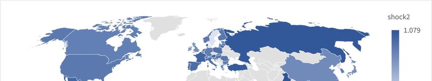
workplace closures.24
We use this extensive set of data to construct our measure for the COVID-19 shock and to
instruct the model to perform counterfactual analysis. As described in section 3, we follow
Dekle et al. (2008) and Caliendo and Parro (2015) and solve the model in relative changes
to identify the welfare effect of the COVID-19 shock. We perform three different exercises:
(i) we include the COVID-19 shock in the model as in equation 1 and we estimate a snap-
shot scenario based on the actual number of COVID-19 cases in each country (Shock-1 in
the tables and figures), (ii) we include the quarantine shock in the model as in equation 2
and estimate a quarantine scenario, imposing quarantine to a fraction of the labour force in
each countries (Shock-2 in the tables and figures), (iii) we decompose the effect into a direct
effect from the production shock induced by the COVID-19 quarantine and an indirect effect
coming from the global shock affecting the other countries. We perform the three exercises
both in an open economy with the actual tariff and trade cost levels and in a closer economy,
where we increase the trade costs by 100 percentage points in each sector-country.

4.1 Open economy

Change in Welfare, Value Added and Trade

In this section, we present the results of the change in welfare, sectoral value added and
trade for each country in our sample and both the snap-shot and the quarantine scenario.
The formula for the welfare change is

 ̂ 
 ̂ =
 
 ∏ =1 ( ̂ )

where ̂ is the change in welfare of country , ̂ is the change in nominal income of
 
country and ∏ =1 ( ̂ ) is the change in the price index for country in each sector .
The aggregated welfare results of the snap-shot and the quarantine scenario by country are
presented in table 1. In column 2 and 5 we present the real income drops from the snap-shot
scenario (shock 1), assuming no quarantine for any country in the world.25 In this case, we

 24 See Hale (2020) for a detailed time-series of government policy responses to the diffusion of the COVID-19
virus.
 25 It is important to highlight that this scenario would however imply a tremendous cost in terms of human
lives that our model does not account for.

 15

find real income drops up to almost 2.9% for Spain, with heterogeneous effects depending
mainly on the actual COVID-19 cases in each country of our sample. In figure 1 we present
graphical evidence on the relation between corona cases and the (log) change in real income
across countries.26
In the quarantine scenario (shock 2) in the open economy in table 1 (columns 3 and 6),
we include quarantine as presented in equation 2. Countries have heterogeneous treatments
depending on the restrictiveness of the policy measures, on the share of workforce employed
in each sector of the economy and on the degree of teleworkability of each sector. Results
in table 1 show that most countries with quarantined labor force experience a drop in real
income above 10%, with the only exception of Sweden. Indeed, Sweden did not implement
any coercive and generalized restriction to the workforce, unless infected with the COVID-19
virus disease.27
In tables 2, we further investigate the sectoral distribution of the economic impact of the
COVID-19 shock. We find that the drop in value added (in billions US dollars) is widespread
across all sectors, but it is especially pronounced for services, intermediate resource manufac-
turing and wholesale and retail trade across all countries and both in the snap-shot scenario
(Shock-1 ) as well as in the quarantine scenario (Shock-2 ). In absolute terms, the strongest
drops in value added are experienced in the services sectors, which include services such as
accommodation and food, real estate, and also public services.28 In relative terms, the drops
in sectoral value added are the highest in the sectors of textiles and electrical equipment
for Italy, pharmaceuticals and motor vehicles for Germany, manufacturing and machinery
equipment for the US and textiles and electrical equipment for China (see table A1 in the
Appendix).

 26 The size of shock 1 across all countries is shown in Appendix A.1 in figure A4 and zooms into the EU
member states in figure A6a.
 27 It is crucial to note that the number of COVID-19 cases as well as the countries that implement quar-
antine is in continuous evolution, hence the point estimates of this scenario might change as the spread of
the COVID-19 disease affects more countries and more people. The focus of this paper is to highlight the
importance of global production networks in the diffusion of a global shock and on how to use a simple
theoretical framework to provide insights on the heterogeneous effects of the COVID-19 shock across coun-
tries and across sector under different scenarios, rather than providing the absolute numbers of the drop in
real income due to the COVID-19 shock. We will constantly update the results of the paper to account for
the new cases as well as for the number of countries in quarantine. The results presented in this version
are supposed to provide a first snap-shot of the economic effect of the COVID-19 shock. A more complete
picture will be available when the full information of COVID-19 cases, quarantined countries and share of
people in quarantine is available.
 28 Table 2 provides the results for selected countries and regions and aggregated sectors. See table A3 for
the aggregation of the 50 WIOD-sectors. All results for the sectoral value added changes for each of the
sectors in all countries can be retrieved from the authors.

 16

The impact of the COVID-19 shock on countries’ trade is presented in table 3. For the case of
Italy, we observe a severe decline in exports in billions US Dollars in intermediate resource
manufacturing, machinery equipment and textiles. Germany faces a decrease in exports
especially marked in the motor vehicle industry, as well as in the intermediate resource
manufacturing sector and machinery and equipment. The US has a severe drop in exports in
the service sector, followed by the intermediate resource manufacturing and wholesales trade
while China experiences the biggest drop in exports in the sectors of electrical equipment,
intermediate resource manufacturing and textiles.
Both the results in tables 2 and 3 present a clear picture of the structure of comparative
advantages of each economy, highlighting the importance of accounting for sectoral produc-
tion linkages and inter-sectoral trade when studying the economic impact of a global shock.
Moreover, these results suggest that the production structure of each economy, as well as
their centrality in the global value chains might have heterogeneous roles in explaining the
size of the observed income drops across the countries.

Decomposition of the Effects

What is the share of the real income drop due to COVID-19 shock that comes from the
disruption of production in each country? What is the share that comes from a drop in
trade through global production networks? To decompose the real income changes observed
in table 1 we use the structural model and perform a counterfactual exercise in which we
shock each country individually. This allows us to isolate the direct production effect of the
COVID-19 shock on each country from the indirect effect that each other country experience
through the global production network. We perform the following decomposition:

 ∀ ≠ ∶ ̂ = ̂ ( ) + ∑ ̂ ( ) × 1 − ̂ ( ) (19)
 ( =1 ) ( )
 ⏟⏞⏞⏞⏞⏞⏞⏞⏞⏞⏟⏞⏞⏞⏞⏞⏞⏞⏞⏞⏟ ⏟⏞⏞⏞⏞⏞⏞⏞⏞⏞⏞⏞⏞⏟⏞⏞⏞⏞⏞⏞⏞⏞⏞⏞⏞⏞⏟ ⏟⏞⏞⏞⏞⏞⏞⏞⏞⏞⏞⏞⏞⏞⏞⏞⏞⏞⏟⏞⏞⏞⏞⏞⏞⏞⏞⏞⏞⏞⏞⏞⏞⏞⏞⏞⏟
 Direct Indirect Global

where ̂ ( ) is the direct ( ) change in real income of country when only country is hit
by the COVID-19 shock ( ), ∑ =1 ̂ ( ) is the sum of the indirect ( ) real income changes
in country when any other country is treated with the COVID-19 shocks ( ), ̂ ( ) is
the total change in real income of country when all countries are affected by the COVID-19
shock ( ), and ̂ is the sum of the three different components from the decomposition.
We perform the decomposition with both Shock-1 and Shock-2.

 17

Suppose, for example, that Germany is the only country hit by the COVID-19 virus disease;
in this case, the real income of Germany would drop because of the disruption in production
that the COVID-19 shock provokes to the German economy, what we call the direct effect
in our decomposition. Suppose now that Italy is the only country affected by the COVID-19
shock. In this case, we would observe a drop in real income for Germany as well, which is
driven by the drop in trade between Germany and Italy, as well as by the increase in the
cost of intermediates that Germany buys from Italy. This is what we call the indirect effect.
Summing over the indirect effects for Germany will provide us the total indirect effect,
namely the drop in real income that Germany faces when each other country is shocked
individually.
The third term of our decomposition is the difference between the sum of the direct and the
indirect effects for Germany from the decomposition and the drop in real income observed
for Germany in the counterfactual exercise in which we shock all the countries at same time.
We call this component the global adjustment. Indeed, when we shock all the countries
with quarantine at the same time, the observed income drop differs from the sum of the
direct and the indirect effect from the decomposition. This points to the importance of
using a GE framework with input-output linkages and trade when studying the effect of
a global shock to local economies. In fact, when shocked all together, each country keeps
the relative importance in the world trade networks, hence the structure of comparative
advantages remains the same and the total effect of the shock is smaller for each of them.
On the contrary, when only one country is hit by the COVID-19 shock, that country faces an
increase in the production costs of the goods produced for the domestic and for the foreign
markets and loses its role in the global production networks, thus experiencing an additional
drop in income.
Figures 2 and 3 present a graphical representation of each part of the decomposition for the
snap-shot scenario (Shock-1 ) as well as for the quarantine scenario (Shock-2 ). Figure 2 and
table 4 present the results for the snap-shot scenario (Shock-1 ): we observe a marked het-
erogeneity both in the total size of the income drop, but also in the share of each component
of the the decomposition. Without quarantine, the total income drop would be between 3%
(Spain) and 0.1% (India). Moreover, the share of the total shock that is accounted for by
the indirect effect varies substantially across countries, accounting for the biggest shares in
countries that have a smaller number of COVID-19 cases, thus experiencing a smaller direct
effect due to disruption in production.
Figure 3 and table 5 show the results of the decomposition for the quarantine scenario (Shock-
2 ). In this case, each country is hit by a shock that accounts for the restrictiveness of the

 18

policy implemented as explained in section 2. It is straightforward to notice the heterogeneity
in the relative importance of the direct as well as the indirect components of the shock across
countries. Moreover, the share of the total drop in real income accounted for by the direct
effect is systematically higher for European countries than for the other countries in our
sample, with the exceptions of Korea and Taiwan. To better understand the heterogeneities
observed in figure 3 and table 5, we construct a simple measure of trade openness as the sum
of imports and exports over total income of the country ( + 
 
 ). Using the data from the
baseline economy and the results of counterfactual economy, we investigate if our measure
of openness is correlated with a higher indirect effect. We estimate the following model:

 + 
 ∑ ̂ ( ) = 0 + 1 + 2 ̂ + 3 _ + 4 _ + + (20)
 =1
 
 2
where _ = ∑ =1 ( ∑ ) ∀ ≠ is an Herfindahl index of diversification in trade
 =1 
partners. The fraction shows the imports of country , from origin country , over the
sum of all Imports of country ; the higher the number of trading partners and the more
diversified its importing sources are, the lower is the HHI of diversification. _ =
 2
 
∑ =1 ( ∑ 
 ) ∀ ≠ is an index of specialization in production. The fraction within the
 =1 
brackets presents the output in sector , in country , over the total output of country . The
higher the HHI of specialization, the lower is the degree of specialization in the country.29
Table 7 presents the results of this exercise. Indeed, countries with a higher degree of open-
ness experience a higher indirect effect. Moreover, accounting for initial income and total
size of the real income drop allows us to have a robust estimation across all columns. This
simple exercise confirms that openness is correlated with a higher global production network
shock; in fact, countries that rely more on international partners both for intermediate sup-
plies as well as for exporting their goods experience a higher indirect shock. It is important
to clarify that this exercise compares countries with different degrees of openness conditional
on receiving the same drop in real income. However, it does not allow us to answer the fol-
lowing counterfactual question: "what would have happened if the world was less integrated?
Would the total drop in real income due to the COVID-19 be smaller in a less integrated
world? In the next section, we leverage on our model to answer these questions.

 29 Similarly,we construct an index of diversification of exports. Results using the index of diversification
of exports are similar to the ones using the diversification in imports.

 19

4.2 Less Integrated World

In this section we quantify the real income effect of the COVID-19 shock in a less integrated
world scenario, where we increase the trade costs in each country and sector by a 100
percentage points. First and unsurprisingly, a less integrated world itself implies enormous
income losses for all countries in our sample. Tables 8 and 9 show the real income changes
for all countries in the sample for shock-1 and shock-2 in a less integrated world. In both
tables, column 2 and 7 present the real income losses stemming from the increase in trade
costs by a 100 percentage points. Column 3 and 8 show the real income changes stemming
from the COVID-19 shocks in a less integrated economy, while columns 4 and 9 present the
welfare effects due to the COVID-19 shocks in the open economy (as in table 1). Finally,
columns 5 and 10 (Δ Shock 1 and Δ Shock2) present the difference between the real income
drop due to the COVID-19 shocks in a less integrated vs. open economy.
The COVID19 shock is smaller for all countries in the less integrated economy than in the
open economy under both shocks. Indeed, in a less integrated world countries experience an
enormous reduction in real income due to the increase in trade costs, hence the additional
effect of the global pandemic shock plays a relatively smaller role. Indeed, in tables 12 and
13, we present the results of the decomposition from equation 19 in a less integrated world.
Interestingly, when raising trade costs in all countries, the indirect component is lower that
in open economy, but it still accounts for a relevant share of the drop in income due to the
COVID-19 shock. In our counterfactual exercise, the increase in trade cost mimics a world
with higher trade barriers, but not a complete autarky scenario; countries would still trade,
use intermediates from abroad and sell final goods in foreign countries.
This finding highlights the importance of inter-sectoral linkages in the transmission of the
shock: a higher degree of integration in the global production network implies that a shock
in one country directly diffuses though the trade linkages to other countries. Trade has
two different effects in our model: on the one hand, it smooths the effect of the shock
by allowing consumers to purchase and consume goods they wouldn’t otherwise be able
to consume in a world with production barriers in quarantine. On the other hand, the
COVID-19 shock increases production costs of intermediate inputs that are used at home
and abroad. Our counterfactual exercise clearly shows that an increase in trade costs would
not significantly decrease the impact of the COVID-19 shock across countries. However,
increasing trade barriers would imply an additional drop in real income between 14% and
33% across countries.

 20

5 Conclusions

This study extends the general equilibrium framework developed by Caliendo and Parro
(2015) to evaluate the economic impact of the COVID-19 shock. We model the COVID-
19 shock as a production barrier that deters production for home consumption and for
exports through a temporary drop in the labor units available in each country. The spread
of COVID-19 disease provides a unique set-up to understand and study the diffusion of a
global production shock along the global value chains. However, understanding the effects of
a global production disruption induced by a pandemic is complex. In this paper, the modeling
choice of the shock takes into account the geography of the diffusion of the COVID-19 shock
across regions and countries, the geographical distribution of sectors in each country and
the labour intensity of each sector of production to return a reliable measure of the impact
of the COVID-19 disease as a production barrier. Crucially, in a model with interrelated
sectors the cost of the input bundle depends on wages and on the price of all the composite
intermediate goods in the economy, both non-tradable and tradable. In our framework, the
COVID-19 shock has a direct effect on the cost of each input as well as an indirect effect via
the sectoral linkages.
We perform three different exercises: (i) we include the COVID-19 shock in the model and
we estimate a snap-shot scenario based on the actual number of COVID-19 cases in each
country, (ii) we include the quarantine shock and estimate a quarantine scenario, imposing
quarantine to a fraction of the labour force in each countries, (iii) we decompose the effect
into a direct effect from the production shock induced by the COVID-19 quarantine and
an indirect effect coming from the global shock affecting the other countries. We perform
the three exercises both in an open economy with the actual tariff and trade cost levels and
in a closer economy, where we increase the trade costs by 100 percentage points in each
sector-country. The quantitative exercise requires data on bilateral trade flows, production,
tariffs, sectoral trade elasticities, employment shares by sector and region and the number
of COVID-19 cases in each region or country. We calibrate a 40 countries 50 sector economy
and incorporate the COVID-19 shock to evaluate the welfare effects for each country both
in aggregate and at the sectoral level.
We show that the shock dramatically reduces real income for all countries in all counterfac-
tual scenarios and that sectoral interrelations and global trade linkages have a crucial role in
explaining the transmission of the shock across countries. COVID-19 shock is a pandemic
shock, hence it has a contemporaneous effect in many countries and to all sectors of produc-
tion. We use the model to perform a model-based identification of the effect of COVID-19

 21

shock and provide evidence on the importance of global trade linkages and inter-sectoral
trade when studying the effect of a global shock to production on the welfare of each coun-
try. Certainly, this model abstract from many other aspects related to the diffusion of the
COVID-19 disease which are the topic of study of epidemiologist, medical doctors and statis-
ticians. Moreover, we do not account for the health consequences of the pandemic itself. We
believe that understanding how the COVID-19 virus disease spreads across regions is outside
the scope of this paper. In our framework, the spread of COVID-19 disease is modeled an
exogenous shock that allows us to study the diffusion of the production disruption along
the global value chains and to highlight the importance of modeling and including sectoral
interrelations to quantify the economic impact of the COVID-19 shock.

 22

References
Alfaro, L., Antràs, P., Chor, D., Conconi, P., 2019. Internalizing global value chains: A
 firm-level analysis. Journal of Political Economy 127, 509–559. URL: https://www.
 journals.uchicago.edu/doi/10.1086/700935.

Altomonte, C, F.D.M.G.O.A.R., Vicard, V., 2012. Global value chains during the great trade
 collapse: a bullwhip effect? Firms in the international economy: Firm heterogeneity
 meets international business .

Antràs, P., Forthcoming. Conceptual aspects of global value chains. World Bank Economic
 Review .

Antràs, P., Chor, D., 2013. Organizing the global value chain. Econometrica 81, 2127–2204.
 URL: http://onlinelibrary.wiley.com/doi/10.3982/ECTA10813/abstract. from
 March 2013.

Antràs, P., Chor, D., 2018. On the Measurement of Upstreamness and Downstreamness in
 Global Value Chains. Taylor & Francis Group. pp. 126–194.

Antràs, P., de Gortari, A., Forthcoming. On the geography of global value chains.

Arkolakis, C., Costinot, A., Rodríguez-Clare, A., 2012. New trade models, same old gains?
 American Economic Review 102, 94–130. URL: http://www.aeaweb.org/articles?
 id=10.1257/aer.102.1.94, doi:10.1257/aer.102.1.94.

Atkeson, A., 2020. What Will Be the Economic Impact of COVID-19 in the US? Rough
 Estimates of Disease Scenarios. Working Paper 26867. National Bureau of Economic
 Research. URL: http://www.nber.org/papers/w26867, doi:10.3386/w26867.

Barrot, J.N., Sauvagnat, J., 2016. Input Specificity and the Propagation of Idiosyncratic
 Shocks in Production Networks *. The Quarterly Journal of Economics 131, 1543–1592.
 URL: https://doi.org/10.1093/qje/qjw018, doi:10.1093/qje/qjw018.

Bénassy-Quéré, A, Y.D.L.F., Khoudour-Casteras, D., 2009. Economic crisis and global
 supply chains. Mimeo .

Berger, D., H.K.M.S., 2020. An seir infectious disease model with testing and conditional
 quarantine. Mimeo .

Boehm, C.E., Flaaen, A., Pandalai-Nayar, N., 2019. Input linkages and the transmission of
 shocks: Firm-level evidence from the 2011 tōhoku earthquake. The Review of Economics
 and Statistics 101, 60–75.

Bombardini, M., Li, B., 2016. Trade, Pollution and Mortality in China. Working Paper
 22804. National Bureau of Economic Research. URL: http://www.nber.org/papers/
 w22804, doi:10.3386/w22804.

 23