Semantic Sentence Matching with Densely-connected Recurrent and Co-attentive Information
←
→
Page content transcription
If your browser does not render page correctly, please read the page content below
Semantic Sentence Matching with Densely-connected
                                                                      Recurrent and Co-attentive Information
                                                                                Seonhoon Kim1,2 , Inho Kang1 , Nojun Kwak2
                                                                                        1
                                                                                            Naver Search, 2 Seoul National University

                                                               {seonhoon.kim|once.ihkang}@navercorp.com, nojunk@snu.ac.kr
arXiv:1805.11360v2 [cs.CL] 2 Nov 2018

                                                                    Abstract                                       et al. 2015), and MultiNLI (Williams, Nangia, and Bowman
                                                                                                                   2017) have contributed significantly to learning semantics as
                                          Sentence matching is widely used in various natural language
                                          tasks such as natural language inference, paraphrase identifica-         well. In the conventional methods, a matching model can be
                                          tion, and question answering. For these tasks, understanding             trained in two different ways (Gong, Luo, and Zhang 2018).
                                          logical and semantic relationship between two sentences is               The first methods are sentence-encoding-based ones where
                                          required but it is yet challenging. Although attention mech-             each sentence is encoded to a fixed-sized vector in a complete
                                          anism is useful to capture the semantic relationship and to              isolated manner and the two vectors for the corresponding
                                          properly align the elements of two sentences, previous meth-             sentences are used in predicting the degree of matching. The
                                          ods of attention mechanism simply use a summation operation              others are joint methods that allow to utilize interactive fea-
                                          which does not retain original features enough. Inspired by              tures like attentive information between the sentences.
                                          DenseNet, a densely connected convolutional network, we
                                          propose a densely-connected co-attentive recurrent neural net-              In the former paradigm, because two sentences have no
                                          work, each layer of which uses concatenated information of               interaction, they can not utilize interactive information dur-
                                          attentive features as well as hidden features of all the preced-         ing the encoding procedure. In our work, we adopted a joint
                                          ing recurrent layers. It enables preserving the original and the         method which enables capturing interactive information for
                                          co-attentive feature information from the bottommost word                performance improvements. Furthermore, we employ a sub-
                                          embedding layer to the uppermost recurrent layer. To alleviate           stantially deeper recurrent network for sentence matching
                                          the problem of an ever-increasing size of feature vectors due            like deep neural machine translator (NMT) (Wu et al. 2016).
                                          to dense concatenation operations, we also propose to use an             Deep recurrent models are more advantageous for learning
                                          autoencoder after dense concatenation. We evaluate our pro-              long sequences and outperform the shallower architectures.
                                          posed architecture on highly competitive benchmark datasets
                                          related to sentence matching. Experimental results show that
                                                                                                                   However, the attention mechanism is unstable in deeper mod-
                                          our architecture, which retains recurrent and attentive features,        els with the well-known vanishing gradient problem. Though
                                          achieves state-of-the-art performances for most of the tasks.            GNMT (Wu et al. 2016) uses residual connection between
                                                                                                                   recurrent layers to allow better information and gradient flow,
                                                                                                                   there are some limitations. The recurrent hidden or attentive
                                                                Introduction                                       features are not preserved intact through residual connection
                                        Semantic sentence matching, a fundamental technology in                    because the summation operation may impede the informa-
                                        natural language processing, requires lexical and composi-                 tion flow in deep networks.
                                        tional semantics. In paraphrase identification, sentence match-               Inspired by Densenet (Huang et al. 2017), we propose a
                                        ing is utilized to identify whether two sentences have identical           densely-connected recurrent network where the recurrent hid-
                                        meaning or not. In natural language inference also known                   den features are retained to the uppermost layer. In addition,
                                        as recognizing textual entailment, it determines whether a                 instead of the conventional summation operation, the con-
                                        hypothesis sentence can reasonably be inferred from a given                catenation operation is used in combination with the attention
                                        premise sentence. In question answering, sentence matching                 mechanism to preserve co-attentive information better. The
                                        is required to determine the degree of matching 1) between a               proposed architecture shown in Figure 1 is called DRCN
                                        query and a question for question retrieval, and 2) between                which is an abbreviation for Densely-connected Recurrent
                                        a question and an answer for answer selection. However                     and Co-attentive neural Network. The proposed DRCN can
                                        identifying logical and semantic relationship between two                  utilize the increased representational power of deeper re-
                                        sentences is not trivial due to the problem of the semantic                current networks and attentive information. Furthermore, to
                                        gap (Liu et al. 2016).                                                     alleviate the problem of an ever-increasing feature vector
                                           Recent advances of deep neural network enable to learn                  size due to concatenation operations, we adopted an autoen-
                                        textual semantics for sentence matching. Large amount of an-               coder and forwarded a fixed length vector to the higher layer
                                        notated data such as Quora (Csernai 2017), SNLI (Bowman                    recurrent module as shown in the figure. DRCN is, to our
                                        Copyright c 2019, Association for the Advancement of Artificial            best knowledge, the first generalized version of DenseRNN
                                        Intelligence (www.aaai.org). All rights reserved.                          which is expandable to deeper layers with the property of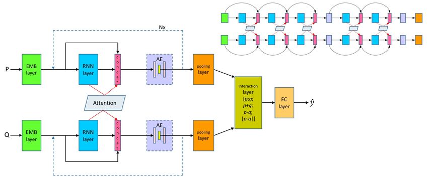
Figure 1: General architecture of our Densely-connected Recurrent and Co-attentive neural Network (DRCN). Dashed arrows
indicate that a group of RNN-layer, concatenation and AE can be repeated multiple (N ) times (like a repeat mark in a music
score). The bottleneck component denoted as AE, inserted to prevent the ever-growing size of a feature vector, is optional for
each repetition. The upper right diagram is our specific architecture for experiments with 5 RNN layers (N = 4).

controllable feature sizes by the use of an autoencoder.          et al. 2017). On the other hand, the joint methods, which
   We evaluate our model on three sentence matching tasks:        make up for the lack of interaction in the former methods,
natural language inference, paraphrase identification and an-     use cross-features as an attention mechanism to express the
swer sentence selection. Experimental results on five highly      word- or phrase-level alignments for performance improve-
competitive benchmark datasets (SNLI, MultiNLI, QUORA,            ments (Wang, Hamza, and Florian 2017; Chen et al. 2017b;
TrecQA and SelQA) show that our model significantly out-          Gong, Luo, and Zhang 2018; Yang et al. 2016).
performs the current state-of-the-art results on most of the         Recently, the architectural developments using deeper lay-
tasks.                                                            ers have led more progress in performance. The residual
                                                                  connection is widely and commonly used to increase the
                     Related Work                                 depth of a network stably (He et al. 2016; Wu et al. 2016).
                                                                  More recently, Huang et al. (Huang et al. 2017) enable the
Earlier approaches of sentence matching mainly relied on          features to be connected from lower to upper layers using the
conventional methods such as syntactic features, transfor-        concatenation operation without any loss of information on
mations or relation extraction (Romano et al. 2006; Wang,         lower-layer features.
Smith, and Mitamura 2007). These are restrictive in that they        External resources are also used for sentence matching.
work only on very specific tasks.                                 Chen et al. (Chen et al. 2017a; Chen et al. 2017b) used syn-
   The developments of large-scale annotated datasets (Bow-       tactic parse trees or lexical databases like WordNet to mea-
man et al. 2015; Williams, Nangia, and Bowman 2017)               sure the semantic relationship among the words and Pavlick
and deep learning algorithms have led a big progress on           et al. (Pavlick et al. 2015) added interpretable semantics to
matching natural language sentences. Furthermore, the well-       the paraphrase database.
established attention mechanisms endowed richer informa-             Unlike these, in this paper, we do not use any such external
tion for sentence matching by providing alignment and             resources. Our work belongs to the joint approaches which
dependency relationship between two sentences. The re-            uses densely-connected recurrent and co-attentive informa-
lease of the large-scale datasets also has encouraged the         tion to enhance representation power for semantic sentence
developments of the learning-centered approaches to se-           matching.
mantic representation. The first type of these approaches
is sentence-encoding-based methods (Conneau et al. 2017;
Choi, Yoo, and goo Lee 2017; Nie and Bansal 2017;
                                                                                             Methods
Shen et al. 2018) where sentences are encoded into their own      In this section, we describe our sentence matching archi-
sentence representation without any cross-interaction. Then,      tecture DRCN which is composed of the following three
a classifier such as a neural network is applied to decide the    components: (1) word representation layer, (2) attentively
relationship based on these independent sentence represen-        connected RNN and (3) interaction and prediction layer. We
tations. These sentence-encoding-based methods are simple         denote two input sentences as P = {p1 , p2 , · · · , pI } and
to extract sentence representation and are able to be used for    Q = {q1 , q2 , · · · , qJ } where pi /qj is the ith /j th word of the
transfer learning to other natural language tasks (Conneau        sentence P /Q and I/J is the word length of P /Q. The overall
architecture of the proposed DRCN is shown in Fig. 1.                 To encourage gradient to flow in the backward pass, resid-
                                                                    ual connection (He et al. 2016) is introduced which bypasses
Word Representation Layer                                           the non-linear transformations with an identity mapping. In-
To construct the word representation layer, we concatenate          corporating this into (2), it becomes
word embedding, character representation and the exact
                                                                                         hlt = Hl (xlt , hlt−1 )
matched flag which was used in (Gong, Luo, and Zhang                                                                            (3)
2018).                                                                                   xlt = hl−1
                                                                                                t   + xl−1
                                                                                                       t .
   In word embedding, each word is represented as a d-
                                                                       However, the summation operation in the residual connec-
dimensional vector by using a pre-trained word embedding
                                                                    tion may impede the information flow in the network (Huang
method such as GloVe (Pennington, Socher, and Manning
                                                                    et al. 2017). Motivated by Densenet (Huang et al. 2017), we
2014) or Word2vec (Mikolov et al. 2013). In our model,
                                                                    employ direct connections using the concatenation operation
a word embedding vector can be updated or fixed during
                                                                    from any layer to all the subsequent layers so that the features
training. The strategy whether to make the pre-trained word
                                                                    of previous layers are not to be modified but to be retained
embedding be trainable or not is heavily task-dependent.
                                                                    as they are as depicted in Figure 1. The densely connected
Trainable word embeddings capture the characteristics of the
                                                                    recurrent neural networks can be described as
training data well but can result in overfitting. On the other
hand, fixed (non-trainable) word embeddings lack flexibility                             hlt = Hl (xlt , hlt−1 )
on task-specific data, while it can be robust for overfitting,                                                                  (4)
                                                                                         xlt = [hl−1  l−1
                                                                                                 t ; xt ].
especially for less frequent words. We use both the trainable
embedding etr                                              f ix
              pi and the fixed (non-trainable) embedding epi        The concatenation operation enables the hidden features to be
to let them play complementary roles in enhancing the perfor-       preserved until they reach to the uppermost layer and all the
mance of our model. This technique of mixing trainable and          previous features work for prediction as collective knowledge
non-trainable word embeddings is simple but yet effective.          (Huang et al. 2017).
   The character representation cpi is calculated by feeding
randomly initialized character embeddings into a convolu-           Densely-connected Co-attentive networks
tional neural network with the max-pooling operation. The           Attention mechanism, which has largely succeeded in many
character embeddings and convolutional weights are jointly          domains (Wu et al. 2016; Vaswani et al. 2017), is a tech-
learned during training.                                            nique to learn effectively where a context vector is matched
   Like (Gong, Luo, and Zhang 2018), the exact match flag           conditioned on a specific sequence.
fpi is activated if the same word is found in the other sen-           Given two sentences, a context vector is calculated based
tence.                                                              on an attention mechanism focusing on the relevant part
   Our final word representational feature pwi for the word pi      of the two sentences at each RNN layer. The calculated at-
is composed of four components as follows:                          tentive information represents soft-alignment between two
             etr    tr
                                    efpiix = E f ix (pi )           sentences. In this work, we also use an attention mechanism.
              pi = E (pi ),
                                                                    We incorporate co-attentive information into densely con-
                    cpi = Char-Conv(pi )                     (1)    nected recurrent features using the concatenation operation,
                  pw   =   [etr   f ix                              so as not to lose any information (Fig. 1). This concatenated
                   i         pi ;epi ; cpi ; fpi ].
                                                                    recurrent and co-attentive features which are obtained by
Here, E tr and E f ix are the trainable and non-trainable (fixed)   densely connecting the features from the undermost to the
word embeddings respectively. Char-Conv is the character-           uppermost layers, enrich the collective knowledge for lexical
level convolutional operation and [· ; ·] is the concatenation      and compositional semantics.
operator. For each word in both sentences, the same above              The attentive information api of the ith word pi ∈ P
procedure is used to extract word features.                         against the sentence Q is calculated as a weighted sum of
                                                                    hqj ’s which are weighted by the softmax weights as follows :
Densely connected Recurrent Networks
                                                                                               J
The ordinal stacked RNNs (Recurrent Neural Networks) are                                       X
composed of multiple RNN layers on top of each other, with                             api =         αi,j hqj
                                                                                               j=1
the output sequence of previous layer forming the input se-
quence for the next. More concretely, let Hl be the lth RNN                                      exp(ei,j )                     (5)
layer in a stacked RNN. Note that in our implementation, we                           αi,j = PJ
                                                                                                k=1 exp(ei,k )
employ the bidirectional LSTM (BiLSTM) as a base block of
Hl . At the time step t, an ordinal stacked RNN is expressed                          ei,j = cos(hpi , hqj )
as follows:                                                            Similar to the densely connected RNN hidden features, we
                      hlt =Hl (xlt , hlt−1 )                        concatenate the attentive context vector api with triggered
                                                         (2)        vector hpi so as to retain attentive information as an input to
                          xlt = hl−1
                                 t .                                the next layer:
While this architecture enables us to build up higher level
representation, deeper networks have difficulties in training                         hlt = Hl (xlt , hlt−1 )
                                                                                                                                (6)
due to the exploding or vanishing gradient problem.                                   xlt = [hl−1  l−1  l−1
                                                                                              t ; at ; xt ].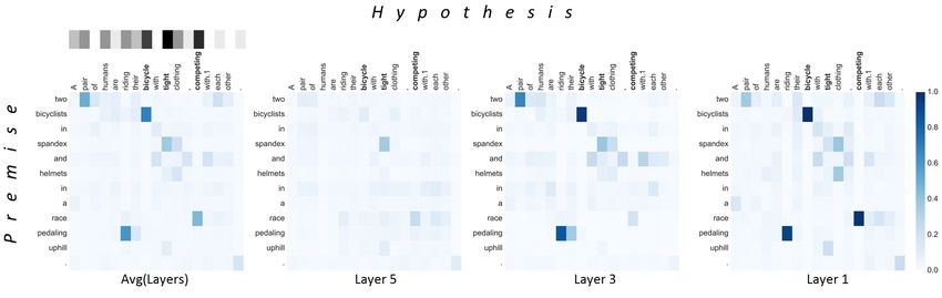
Bottleneck component                                                Premise two bicyclists in spandex and helmets in a
Our network uses all layers’ outputs as a community of se-          race pedaling uphill.
mantic knowledge. However, this network is a structure with         Hypothesis A pair of humans are riding their bicy-
increasing input features as layers get deeper, and has a large     cle with tight clothing, competing with each other.
number of parameters especially in the fully-connected layer.       Label {entailment; neutral; contradiction}
To address this issue, we employ an autoencoder as a bottle-        Premise Several men in front of a white building.
neck component. Autoencoder is a compression technique              Hypothesis Several people in front of a gray build-
that reduces the number of features while retaining the orig-       ing.
inal information, which can be used as a distilled semantic         Label {entailment; neutral; contradiction}
knowledge in our model. Furthermore, this component in-
creased the test performance by working as a regularizer in            Table 1: Examples of natural language inference.
our experiments.

Interaction and Prediction Layer                                  units. We set 1000 hidden units with respect to the fully-
To extract a proper representation for each sentence, we apply    connected layers. The dropout was applied after the word
the step-wise max-pooling operation over densely connected        and character embedding layers with a keep rate of 0.5. It
recurrent and co-attentive features (pooling in Fig. 1). More     was also applied before the fully-connected layers with a
specifically, if the output of the final RNN layer is a 100d      keep rate of 0.8. For the bottleneck component, we set 200
vector for a sentence with 30 words, a 30 × 100 matrix is         hidden units as encoded features of the autoencoder with a
obtained which is max-pooled column-wise such that the size       dropout rate of 0.2. The batch normalization was applied on
of the resultant vector p or q is 100. Then, we aggregate these   the fully-connected layers, only for the one-way type datasets.
representations p and q for the two sentences P and Q in var-     The RMSProp optimizer with an initial learning rate of 0.001
ious ways in the interaction layer and the final feature vector   was applied. The learning rate was decreased by a factor of
v for semantic sentence matching is obtained as follows:          0.85 when the dev accuracy does not improve. All weights
                                                                  except embedding matrices are constrained by L2 regulariza-
              v = [p; q; p + q; p − q; |p − q|].           (7)    tion with a regularization constant λ = 10−6 . The sequence
Here, the operations +, − and | · | are performed element-        lengths of the sentence are all different for each dataset: 35
wise to infer the relationship between two sentences. The         for SNLI, 55 for MultiNLI, 25 for Quora question pair and 50
element-wise subtraction p − q is an asymmetric operator          for TrecQA. The learning parameters were selected based on
for one-way type tasks such as natural language inference or      the best performance on the dev set. We employed 8 different
answer sentence selection.                                        randomly initialized sets of parameters with the same model
                                                                  for our ensemble approach.
   Finally, based on previously aggregated features v, we use
two fully-connected layers with ReLU activation followed
by one fully-connected output layer. Then, the softmax func-      Experimental Results
tion is applied to obtain a probability distribution of each      SNLI and MultiNLI We evaluated our model on the natu-
class. The model is trained end-to-end by minimizing the          ral language inference task over SNLI and MultiNLI datasets.
multi-class cross entropy loss and the reconstruction loss of     Table 2 shows the results on SNLI dataset of our model with
autoencoders.                                                     other published models. Among them, ESIM+ELMo and LM-
                                                                  Transformer are the current state-of-the-art models. However,
                      Experiments                                 they use additional contextualized word representations from
                                                                  language models as an externel knowledge. The proposed
We evaluate our matching model on five popular and well-          DRCN obtains an accuracy of 88.9% which is a competitive
studied benchmark datasets for three challenging sentence         score although we do not use any external knowledge like
matching tasks: (i) SNLI and MultiNLI for natural language        ESIM+ELMo and LM-Transformer. The ensemble model
inference; (ii) Quora Question Pair for paraphrase identifi-      achieves an accuracy of 90.1%, which sets the new state-of-
cation; and (iii) TrecQA and SelQA for answer sentence            the-art performance. Our ensemble model with 53m parame-
selection in question answering. Additional details about the     ters (6.7m×8) outperforms the LM-Transformer whose the
above datasets can be found in the supplementary materials.       number of parameters is 85m. Furthermore, in case of the
                                                                  encoding-based method, we obtain the best performance of
Implementation Details                                            86.5% without the co-attention and exact match flag.
We initialized word embedding with 300d GloVe vectors                Table 3 shows the results on MATCHED and MISMATCHED
pre-trained from the 840B Common Crawl corpus (Penning-           problems of MultiNLI dataset. Our plain DRCN has a com-
ton, Socher, and Manning 2014), while the word embeddings         petitive performance without any contextualized knowledge.
for the out-of-vocabulary words were initialized randomly.        And, by combining DRCN with the ELMo, one of the con-
We also randomly initialized character embedding with a           textualized embeddings from language models, our model
16d vector and extracted 32d character representation with a      outperforms the LM-Transformer which has 85m parameters
convolutional network. For the densely-connected recurrent        with fewer parameters of 61m. From this point of view, the
layers, we stacked 5 layers each of which have 100 hidden         combination of our model with a contextualized knowledge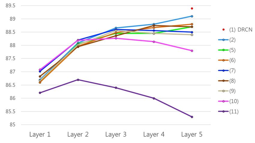
Models                                                  Acc.          |θ|    Models                                          Accuracy (%)
                    Sentence encoding-based method                            Siamese-LSTM (Wang, Hamza, and Florian 2017)       82.58
 BiLSTM-Max (Conneau et al. 2017)                        84.5       40m       MP LSTM (Wang, Hamza, and Florian 2017)            83.21
 Gumbel TreeLSTM (Choi, Yoo, and goo Lee 2017)           85.6       2.9m      L.D.C. (Wang, Hamza, and Florian 2017)             85.55
 CAFE (Tay, Tuan, and Hui 2017)                          85.9       3.7m      BiMPM (Wang, Hamza, and Florian 2017)              88.17
 Gumbel TreeLSTM (Choi, Yoo, and goo Lee 2017)           86.0       10m       pt-DecAttchar.c (Tomar et al. 2017)                88.40
 Residual stacked (Nie and Bansal 2017)                  86.0       29m       DIIN (Gong, Luo, and Zhang 2018)                   89.06
 Reinforced SAN (Shen et al. 2018)                       86.3       3.1m
                                                                              DRCN                                               90.15
 Distance SAN (Im and Cho 2017)                          86.3       3.1m
 DRCN (- Attn, - Flag)                                   86.5       5.6m      DIIN* (Gong, Luo, and Zhang 2018)                  89.84
                 Joint method (cross-features available)                      DRCN*                                              91.30
 DIIN (Gong, Luo, and Zhang 2018)                     88.0 / 88.9   4.4m
 ESIM (Chen et al. 2017b)                             88.0 / 88.6   4.3m     Table 4: Classification accuracy for paraphrase identification
 BCN+CoVe+Char (McCann et al. 2017)                   88.1 / -      22m      on Quora question pair test set. * denotes ensemble methods.
 DR-BiLSTM (Ghaeini et al. 2018)                      88.5 / 89.3   7.5m
 CAFE (Tay, Tuan, and Hui 2017)                       88.5 / 89.3   4.7m
 KIM (Chen et al. 2017a)                              88.6 / 89.1   4.3m       Models                                        MAP       MRR
 ESIM+ELMo (Peters et al. 2018)                       88.7 / 89.3   8.0m                              Raw version
 LM-Transformer (Radford et al. 2018)                 89.9 / -      85m
 DRCN (- AE)                                          88.7 / -      20m        aNMM (Yang et al. 2016)                        0.750    0.811
 DRCN                                                 88.9 / 90.1   6.7m       PWIM (He and Lin 2016)                         0.758    0.822
                                                                               MP CNN (He, Gimpel, and Lin 2015)              0.762    0.830
Table 2: Classification accuracy (%) for natural language                      HyperQA (Tay, Luu, and Hui 2017)               0.770    0.825
inference on SNLI test set. |θ| denotes the number of param-                   PR+CNN (Rao, He, and Lin 2016)                 0.780    0.834
eters in each model.                                                           DRCN                                           0.804    0.862
                                                                                                     clean version
                                                    Accuracy (%)               HyperQA (Tay, Luu, and Hui 2017)               0.801    0.877
 Models
                                              MATCHED      MISMATCHED          PR+CNN (Rao, He, and Lin 2016)                 0.801    0.877
 ESIM (Williams, Nangia, and Bowman 2017)        72.3           72.1           BiMPM (Wang, Hamza, and Florian 2017)          0.802    0.875
 DIIN (Gong, Luo, and Zhang 2018)                78.8           77.8
 CAFE (Tay, Tuan, and Hui 2017)                  78.7           77.9           Comp.-Aggr. (Bian et al. 2017)                 0.821    0.899
 LM-Transformer (Radford et al. 2018)            82.1           81.4           IWAN (Shen, Yang, and Deng 2017)               0.822    0.889
 DRCN                                            79.1           78.4           DRCN                                           0.830    0.908
 DIIN* (Gong, Luo, and Zhang 2018)               80.0           78.7
 CAFE* (Tay, Tuan, and Hui 2017)                 80.2           79.0                            (a) TrecQA: raw and clean
 DRCN*                                           80.6           79.5
 DRCN+ELMo*                                      82.3           81.4
                                                                               Models                                          MAP     MRR
                                                                               CNN-DAN (Santos, Wadhawan, and Zhou 2017)       0.866   0.873
Table 3: Classification accuracy for natural language infer-                   CNN-hinge (Santos, Wadhawan, and Zhou 2017)     0.876   0.881
ence on MultiNLI test set. * denotes ensemble methods.                         ACNN (Shen et al. 2017)                         0.874   0.880
                                                                               AdaQA (Shen et al. 2017)                        0.891   0.898
                                                                               DRCN                                            0.925   0.930
is a good option to enhance the performance.                                                            (b) SelQA
Quora Question Pair Table 4 shows our results on the
                                                                             Table 5: Performance for answer sentence selection on
Quora question pair dataset. BiMPM using the multi-
                                                                             TrecQA and selQA test set.
perspective matching technique between two sentences re-
ports baseline performance of a L.D.C. network and basic
multi-perspective models (Wang, Hamza, and Florian 2017).
We obtained accuracies of 90.15% and 91.30% in single                        ine the effectiveness of our word embedding technique as
and ensemble methods, respectively, surpassing the previous                  well as the proposed densely-connected recurrent and co-
state-of-the-art model of DIIN.                                              attentive features. Firstly, we verified the effectiveness of the
                                                                             autoencoder as a bottleneck component in (2). Although the
TrecQA and SelQA Table 5 shows the performance of                            number of parameters in the DRCN significantly decreased
different models on TrecQA and SelQA datasets for answer                     as shown in Table 2, we could see that the performance was
sentence selection task that aims to select a set of candidate               rather higher because of the regularization effect. Secondly,
answer sentences given a question. Most competitive models                   we study how the technique of mixing trainable and fixed
(Shen, Yang, and Deng 2017; Bian et al. 2017; Wang, Hamza,                   word embeddings contributes to the performance in models
and Florian 2017; Shen et al. 2017) also use attention methods               (3-4). After removing E tr or E f ix in eq. (1), the performance
for words alignment between question and candidate answer                    degraded, slightly. The trainable embedding E tr seems more
sentences. However, the proposed DRCN using collective                       effective than the fixed embedding E f ix . Next, the effective-
attentions over multiple layers, achieves the new state-of-                  ness of dense connections was tested in models (5-9). In (5-6),
the-art performance, exceeding the current state-of-the-art                  we removed dense connections only over co-attentive or re-
performance significantly on both datasets.                                  current features, respectively. The result shows that the dense
                                                                             connections over attentive features are more effective. In (7),
Analysis                                                                     we removed dense connections over both co-attentive and
Ablation study We conducted an ablation study on the                         recurrent features, and the performance degraded to 88.5%.
SNLI dev set as shown in Table 6, where we aim to exam-                      In (8), we replace dense connection with residual connection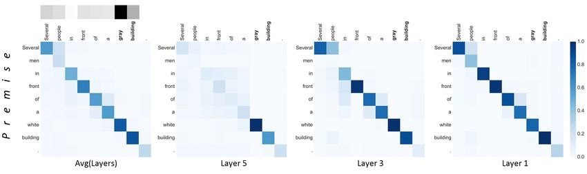
Models                                       Accuracy (%)              Category           ESIM DIIN       CAFE   DRCN
 (1) DRCN                                         89.4                                        Matched
                                                                        Conditional         100      57     70      65
 (2) − autoencoder                                89.1                  Word overlap         50      79     82      89
 (3) − E tr                                       88.7                  Negation             76      78     76      80
 (4) − E f ix                                     88.9                  Antonym              67      82     82      82
 (5) − dense(Attn.)                               88.7                  Long Sentence        75      81     79      83
 (6) − dense(Rec.)                                88.8                  Tense Difference     73      84     82      82
 (7) − dense(Rec. & Attn.)                        88.5                  Active/Passive       88      93    100      87
 (8) − dense(Rec. & Attn.)                                              Paraphrase           89      88     88      92
                                                   88.7                 Quantity/Time        33      53     53      73
     + res(Rec. & Attn.)
                                                                        Coreference          83      77     80      80
 (9) − dense(Rec. & Attn. & Emb)                                        Quantifier           69      74     75      78
                                                   88.4
     + res(Rec. & Attn.)                                                Modal                78      84     81      81
 (10) − dense(Rec. & Attn. & Emb)                  87.8                 Belief               65      77     77      76
 (11) − dense(Rec. & Attn. & Emb) - Attn.          85.3                 Mean                72.8   77.46   78.9    80.6
                                                                        Stddev              16.6   10.75   10.2    6.7
   Table 6: Ablation study results on the SNLI dev sets.                                    Mismatched
                                                                        Conditional          60      69     85      89
                                                                        Word overlap         62      92     87      89
                                                                        Negation             71      77     80      78
                                                                        Antonym              58      80     80      80
                                                                        Long Sentence        69      73     77      84
                                                                        Tense Difference     79      78     89      83
                                                                        Active/Passive       91      70     90     100
                                                                        Paraphrase           84     100     95      90
                                                                        Quantity/Time        54      69     62      80
                                                                        Coreference          75      79     83      87
                                                                        Quantifier           72      78     80      82
                                                                        Modal                76      75     81      87
                                                                        Belief               67      81     83      85
                                                                        Mean                70.6   78.53   82.5    85.7
                                                                        Stddev              10.2    8.55   7.6     5.5

Figure 2: Comparison of models on every layer in ablation        Table 7: Accuracy (%) of Linguistic correctness on MultiNLI
study. (best viewed in color)                                    dev sets.

only over recurrent and co-attentive features. It means that     Word Alignment and Importance Our densely-
only the word embedding features are densely connected to        connected recurrent and co-attentive features are connected
the uppermost layer while recurrent and attentive features are   to the classification layer through the max pooling operation
connected to the upper layer using the residual connection. In   such that all max-valued features of every layer affect the loss
(9), we removed additional dense connection over word em-        function and perform a kind of deep supervision (Huang et al.
bedding features from (8). The results of (8-9) demonstrate      2017). Thus, we could cautiously interpret the classification
that the dense connection using concatenation operation over     results using our attentive weights and max-pooled positions.
deeper layers, has more powerful capability retaining collec-    The attentive weights contain information on how two
tive knowledge to learn textual semantics. The model (10)        sentences are aligned and the numbers of max-pooled
is the basic 5-layer RNN with attention and (11) is the one      positions in each dimension play an important role in
without attention. The result of (10) shows that the connec-     classification.
tions among the layers are important to help gradient flow.         Figure 3 shows the attention map (αi,j in eq. (5)) on each
And, the result of (11) shows that the attentive information     layer of the samples in Table 1. The Avg(Layers) is the aver-
functioning as a soft-alignment is significantly effective in    age of attentive weights over 5 layers and the gray heatmap
semantic sentence matching.                                      right above the Avg(Layers) is the rate of max-pooled posi-
   The performances of models having different number of         tions. The darker indicates the higher importance in classi-
recurrent layers are also reported in Fig. 2. The models (5-9)   fication. In the figure, we can see that tight, competing and
which have connections between layers, are more robust to        bicycle are more important words than others in classifying
the increased depth of network, however, the performances        the label. The word tight clothing in the hypothesis can be
of (10-11) tend to degrade as layers get deeper. In addition,    inferred from spandex in the premise. And competing is also
the models with dense connections rather than residual con-      inferred from race. Other than that, the riding is matched
nections, have higher performance in general. Figure 2 shows     with pedaling, and pair is matched with two. Judging by the
that the connection between layers is essential, especially in   matched terms, the model is undoubtedly able to classify the
deep models, endowing more representational power, and the       label as an entailment, correctly.
dense connection is more effective than the residual connec-        In Figure 3 (b), most of words in both the premise and
tion.                                                            the hypothesis coexist except white and gray. In attention
(a) entailment
(b) contradiction
Figure 3: Visualization of attentive weights and the rate of max-pooled position. The darker, the higher. See supplementary
materials for a comparison with other models that use the residual connections.
map of layer 1, the same or similar words in each sentence Conclusion
have a high correspondence (gray and white are not exactly In this paper, we introduce a densely-connected recurrent and
matched but have a linguistic relevance). However, as the co-attentive network (DRCN) for semantic sentence match-
layers get deeper, the relevance between white building and ing. We connect the recurrent and co-attentive features from
gray building is only maintained as a clue of classification the bottom to the top layer without any deformation. These
(See layer 5). Because white is clearly different from gray, intact features over multiple layers compose a community
our model determines the label as a contradiction. of semantic knowledge and outperform the previous deep
The densely connected recurrent and co-attentive fea- RNN models using residual connections. In doing so, bot-
tures are well-semanticized over multiple layers as collective tleneck components are inserted to reduce the size of the
knowledge. And the max pooling operation selects the soft- network. Our proposed model is the first generalized ver-
positions that may extract the clues on inference correctly. sion of DenseRNN which can be expanded to deeper layers
with the property of controllable feature sizes by the use of
an autoencoder. We additionally show the interpretability of
our model using the attentive weights and the rate of max-
Linguistic Error Analysis We conducted a linguistic error pooled positions. Our model achieves the state-of-the-art
analysis on MultiNLI, and compared DRCN with the ESIM, performance on most of the datasets of three highly challeng-
DIIN and CAFE. We used annotated subset provided by ing natural language tasks. Our proposed method using the
the MultiNLI dataset, and each sample belongs to one of collective semantic knowledge is expected to be applied to
the 13 linguistic categories. The results in table 7 show that the various other natural language tasks.
our model generally has a good performance than others on
most categories. Especially, we can see that ours outperforms References
much better on the Quantity/Time category which is one of [Bian et al. 2017] Bian, W.; Li, S.; Yang, Z.; Chen, G.; and Lin, Z.
the most difficult problems. Furthermore, our DRCN shows 2017. A compare-aggregate model with dynamic-clip attention for
the highest mean and the lowest stddev for both MATCHED answer selection. In Proceedings of the 2017 ACM on Conference
and MISMATCHED problems, which indicates that it not only on Information and Knowledge Management, 1987–1990. ACM.
results in a competitive performance but also has a consistent [Bowman et al. 2015] Bowman, S. R.; Angeli, G.; Potts, C.; and
performance. Manning, C. D. 2015. A large annotated corpus for learningnatural language inference. In Proceedings of the 2015 Conference [Nie and Bansal 2017] Nie, Y., and Bansal, M. 2017. Shortcut-
on Empirical Methods in Natural Language Processing (EMNLP). stacked sentence encoders for multi-domain inference. arXiv
Association for Computational Linguistics. preprint arXiv:1708.02312.
[Chen et al. 2017a] Chen, Q.; Zhu, X.; Ling, Z.-H.; and Inkpen, D. [Pavlick et al. 2015] Pavlick, E.; Bos, J.; Nissim, M.; Beller, C.;
2017a. Natural language inference with external knowledge. arXiv Van Durme, B.; and Callison-Burch, C. 2015. Adding seman-
preprint arXiv:1711.04289. tics to data-driven paraphrasing. In Proceedings of the 53rd Annual
[Chen et al. 2017b] Chen, Q.; Zhu, X.; Ling, Z.-H.; Wei, S.; Jiang, Meeting of the Association for Computational Linguistics and the
H.; and Inkpen, D. 2017b. Enhanced lstm for natural language infer- 7th International Joint Conference on Natural Language Processing
ence. In Proceedings of the 55th Annual Meeting of the Association (Volume 1: Long Papers), volume 1, 1512–1522.
for Computational Linguistics (Volume 1: Long Papers), volume 1, [Pennington, Socher, and Manning 2014] Pennington, J.; Socher,
1657–1668. R.; and Manning, C. D. 2014. Glove: Global vectors for word
[Choi, Yoo, and goo Lee 2017] Choi, J.; Yoo, K. M.; and goo Lee, representation. In Empirical Methods in Natural Language Process-
S. 2017. Learning to compose task-specific tree structures. AAAI. ing (EMNLP), 1532–1543.
[Peters et al. 2018] Peters, M. E.; Neumann, M.; Iyyer, M.; Gardner,
[Conneau et al. 2017] Conneau, A.; Kiela, D.; Schwenk, H.; Bar-
M.; Clark, C.; Lee, K.; and Zettlemoyer, L. 2018. Deep contextual-
rault, L.; and Bordes, A. 2017. Supervised learning of universal
ized word representations. In Proc. of NAACL.
sentence representations from natural language inference data. arXiv
preprint arXiv:1705.02364. [Radford et al. 2018] Radford, A.; Narasimhan, K.; Salimans, T.;
and Sutskever, I. 2018. Improving language understanding by
[Csernai 2017] Csernai, K. 2017. Quora question pair dataset. generative pre-training.
[Ghaeini et al. 2018] Ghaeini, R.; Hasan, S. A.; Datla, V.; Liu, J.; [Rao, He, and Lin 2016] Rao, J.; He, H.; and Lin, J. 2016. Noise-
Lee, K.; Qadir, A.; Ling, Y.; Prakash, A.; Fern, X. Z.; and Farri, O. contrastive estimation for answer selection with deep neural net-
2018. Dr-bilstm: Dependent reading bidirectional lstm for natural works. In Proceedings of the 25th ACM International on Conference
language inference. arXiv preprint arXiv:1802.05577. on Information and Knowledge Management, 1913–1916. ACM.
[Gong, Luo, and Zhang 2018] Gong, Y.; Luo, H.; and Zhang, J. [Romano et al. 2006] Romano, L.; Kouylekov, M.; Szpektor, I.; Da-
2018. Natural language inference over interaction space. In In- gan, I.; and Lavelli, A. 2006. Investigating a generic paraphrase-
ternational Conference on Learning Representations. based approach for relation extraction. In 11th Conference of the
[He and Lin 2016] He, H., and Lin, J. 2016. Pairwise word inter- European Chapter of the Association for Computational Linguistics.
action modeling with deep neural networks for semantic similarity [Santos, Wadhawan, and Zhou 2017] Santos, C. N. d.; Wadhawan,
measurement. In Proceedings of the 2016 Conference of the North K.; and Zhou, B. 2017. Learning loss functions for semi-supervised
American Chapter of the Association for Computational Linguistics: learning via discriminative adversarial networks. arXiv preprint
Human Language Technologies, 937–948. arXiv:1707.02198.
[He et al. 2016] He, K.; Zhang, X.; Ren, S.; and Sun, J. 2016. Deep [Shen et al. 2017] Shen, D.; Min, M. R.; Li, Y.; and Carin, L. 2017.
residual learning for image recognition. In Proceedings of the IEEE Adaptive convolutional filter generation for natural language under-
conference on computer vision and pattern recognition, 770–778. standing. arXiv preprint arXiv:1709.08294.
[He, Gimpel, and Lin 2015] He, H.; Gimpel, K.; and Lin, J. 2015. [Shen et al. 2018] Shen, T.; Zhou, T.; Long, G.; Jiang, J.; Wang, S.;
Multi-perspective sentence similarity modeling with convolutional and Zhang, C. 2018. Reinforced self-attention network: a hybrid
neural networks. In Proceedings of the 2015 Conference on Empiri- of hard and soft attention for sequence modeling. arXiv preprint
cal Methods in Natural Language Processing, 1576–1586. arXiv:1801.10296.
[Huang et al. 2017] Huang, G.; Liu, Z.; Weinberger, K. Q.; and [Shen, Yang, and Deng 2017] Shen, G.; Yang, Y.; and Deng, Z.-H.
van der Maaten, L. 2017. Densely connected convolutional net- 2017. Inter-weighted alignment network for sentence pair modeling.
works. In Proceedings of the IEEE conference on computer vision In Proceedings of the 2017 Conference on Empirical Methods in
and pattern recognition, volume 1, 3. Natural Language Processing, 1179–1189.
[Im and Cho 2017] Im, J., and Cho, S. 2017. Distance-based self- [Tay, Luu, and Hui 2017] Tay, Y.; Luu, A. T.; and Hui, S. C. 2017.
attention network for natural language inference. arXiv preprint Enabling efficient question answer retrieval via hyperbolic neural
arXiv:1712.02047. networks. CoRR abs/1707.07847.
[Jurczyk, Zhai, and Choi 2016] Jurczyk, T.; Zhai, M.; and Choi, J. D. [Tay, Tuan, and Hui 2017] Tay, Y.; Tuan, L. A.; and Hui, S. C. 2017.
2016. Selqa: A new benchmark for selection-based question an- A compare-propagate architecture with alignment factorization for
swering. In Tools with Artificial Intelligence (ICTAI), 2016 IEEE natural language inference. arXiv preprint arXiv:1801.00102.
28th International Conference on, 820–827. IEEE. [Tomar et al. 2017] Tomar, G. S.; Duque, T.; Täckström, O.; Uszko-
[Liu et al. 2016] Liu, P.; Qiu, X.; Chen, J.; and Huang, X. 2016. reit, J.; and Das, D. 2017. Neural paraphrase identification of
Deep fusion lstms for text semantic matching. In Proceedings questions with noisy pretraining. arXiv preprint arXiv:1704.04565.
of the 54th Annual Meeting of the Association for Computational [Vaswani et al. 2017] Vaswani, A.; Shazeer, N.; Parmar, N.; Uszko-
Linguistics (Volume 1: Long Papers), volume 1, 1034–1043. reit, J.; Jones, L.; Gomez, A. N.; Kaiser, Ł.; and Polosukhin, I.
[McCann et al. 2017] McCann, B.; Bradbury, J.; Xiong, C.; and 2017. Attention is all you need. In Advances in Neural Information
Socher, R. 2017. Learned in translation: Contextualized word Processing Systems, 6000–6010.
vectors. In Advances in Neural Information Processing Systems, [Wang, Hamza, and Florian 2017] Wang, Z.; Hamza, W.; and Flo-
6297–6308. rian, R. 2017. Bilateral multi-perspective matching for natural
[Mikolov et al. 2013] Mikolov, T.; Sutskever, I.; Chen, K.; Corrado, language sentences. arXiv preprint arXiv:1702.03814.
G. S.; and Dean, J. 2013. Distributed representations of words [Wang, Smith, and Mitamura 2007] Wang, M.; Smith, N. A.; and
and phrases and their compositionality. In Advances in neural Mitamura, T. 2007. What is the jeopardy model? a quasi-
information processing systems, 3111–3119. synchronous grammar for qa. In Proceedings of the 2007 JointConference on Empirical Methods in Natural Language Processing Visualization on the comparable models
and Computational Natural Language Learning (EMNLP-CoNLL). We study how the attentive weights flow as layers get deeper in each
[Williams, Nangia, and Bowman 2017] Williams, A.; Nangia, N.; model using the dense or residual connection. We used the samples
and Bowman, S. R. 2017. A broad-coverage challenge cor- of the SNLI dev set in Table 1.
pus for sentence understanding through inference. arXiv preprint Figure 4 and 5 show the attention map on each layer of the models
arXiv:1704.05426. of DRCN, Table 6 (8), and Table 6 (9). In the model of Table 6
[Wu et al. 2016] Wu, Y.; Schuster, M.; Chen, Z.; Le, Q. V.; Norouzi, (8), we replaced the dense connection with the residual connection
M.; Macherey, W.; Krikun, M.; Cao, Y.; Gao, Q.; Macherey, K.; only over recurrent and co-attentive features. And, in the model of
et al. 2016. Google’s neural machine translation system: Bridging Table 6 (9), we removed additional dense connection over word
the gap between human and machine translation. arXiv preprint embedding features from Table 6 (8). We denote the model of Table
arXiv:1609.08144. 6 (9) as Res1 and the model of Table 6 (8) as Res2 for convenience.
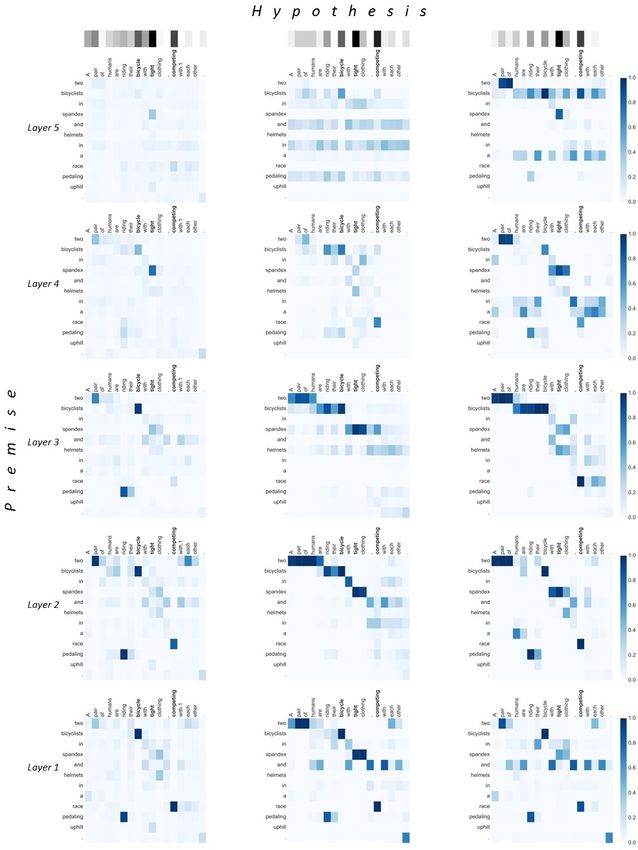
In Figure 4, DRCN does not try to find the right alignments at
[Yang et al. 2016] Yang, L.; Ai, Q.; Guo, J.; and Croft, W. B. 2016.
the upper layer if it already finds the rationale for the prediction
anmm: Ranking short answer texts with attention-based neural
at the relatively lower layer. This is expected that the DRCN use
matching model. In Proceedings of the 25th ACM International on
the features of all the preceding layers as a collective knowledge.
Conference on Information and Knowledge Management, 287–296.
While Res1 and Res2 have to find correct alignments at the top
ACM.
layer, however, there are some misalignments such as competing
and bicyclists rather than competing and race in Res2 model.
Supplementary Material In the second example in Figure 5, although the DRCN couldn’t
Datasets find the clues at the lower layer, it gradually finds the alignments,
which can be a rationale for the prediction. At the 5th layer of
A. SNLI is a collection of 570k human written sentence pairs based
DRCN, the attentive weights of gray building and white building
on image captioning, supporting the task of natural language infer-
are significantly higher than others. On the other hand, the attentive
ence (Bowman et al. 2015). The labels are composed of entailment,
weights are spread in several positions in both Res1 and Res2 which
neutral and contradiction. The data splits are provided in (Bowman
use residual connection.
et al. 2015).
B. MultiNLI, also known as Multi-Genre NLI, has 433k sentence
pairs whose size and mode of collection are modeled closely like
SNLI. MultiNLI offers ten distinct genres (FACE-TO-FACE, TELE-
PHONE, 9/11, TRAVEL, LETTERS, OUP, SLATE, VERBATIM,
GOVERNMENT and FICTION) of written and spoken English data.
Also, there are matched dev/test sets which are derived from the
same sources as those in the training set, and mismatched sets which
do not closely resemble any seen at training time. The data splits
are provided in (Williams, Nangia, and Bowman 2017).
C. Quora Question Pair consists of over 400k question pairs
based on actual quora.com questions. Each pair contains a binary
value indicating whether the two questions are paraphrase or not.
The training-dev-test splits for this dataset are provided in (Wang,
Hamza, and Florian 2017).
D. TrecQA provided in (Wang, Smith, and Mitamura 2007) was
collected from TREC Question Answering tracks 8-13. There are
two versions of data due to different pre-processing methods, namely
clean and raw (Rao, He, and Lin 2016). We evaluate our model on
both data and follow the same data split as provided in (Wang,
Smith, and Mitamura 2007). We use official evaluation metrics of
MAP (Mean Average Precision) and MRR (Mean Reciprocal Rank),
which are standard metrics in information retrieval and question
answering tasks.
E. SelQA consists of questions generated through crowdsourcing
and the answer senteces are extracted from the ten most prevalent
topics (Arts, Country, Food, Historical Events, Movies, Music, Sci-
ence, Sports, Travel and TV) in the English Wikipedia. We also use
MAP and MRR for our evaluation metrics, and the data splits are
provided in (Jurczyk, Zhai, and Choi 2016).Figure 4: Visualization of attentive weights on the entailment example. The premise is “two bicyclists in spandex and helmets in a race pedaling uphill." and the hypothesis is “A pair of humans are riding their bicycle with tight clothing, competing with each other.". The attentive weights of DRCN, Res1, and Res2 are presented from left to right.
Figure 5: Visualization of attentive weights on the contradiction example. The premise is “Several men in front of a white
building." and the hypothesis is “Several people in front of a gray building.". The attentive weights of DRCN, Res1, and Res2 are
presented from left to right.
You can also read