Worldwide Pose Estimation using 3D Point Clouds
←
→
Page content transcription
If your browser does not render page correctly, please read the page content below
Worldwide Pose Estimation using 3D Point Clouds

        Yunpeng Li∗         Noah Snavely†          Dan Huttenlocher†           Pascal Fua∗
                       ∗
                         EPFL {yunpeng.li,pascal.fua}@epfl.ch
                  †
                      Cornell University {snavely,dph}@cs.cornell.edu

         Abstract. We address the problem of determining where a photo was taken
         by estimating a full 6-DOF-plus-intrincs camera pose with respect to a large
         geo-registered 3D point cloud, bringing together research on image localization,
         landmark recognition, and 3D pose estimation. Our method scales to datasets with
         hundreds of thousands of images and tens of millions of 3D points through the
         use of two new techniques: a co-occurrence prior for RANSAC and bidirectional
         matching of image features with 3D points. We evaluate our method on several
         large data sets, and show state-of-the-art results on landmark recognition as well
         as the ability to locate cameras to within meters, requiring only seconds per query.

1     Introduction
Localizing precisely where a photo or video was taken is a key problem in computer
vision with a broad range of applications, including consumer photography (“where did
I take these photos again?”), augmented reality [1], photo editing [2], and autonomous
navigation [3]. Information about camera location can also aid in more general scene
understanding tasks [4, 5]. With the rapid growth of online photo sharing sites and the
creation of more structured image collections such as Google’s Street View, increasingly
any new photo can in principle be localized with respect to this growing set of existing
imagery.
    In this paper, we approach the image localization problem as that of worldwide
pose estimation: given an image, automatically determine a camera matrix (position,
orientation, and camera intrinsics) in a georeferenced coordinate system. As such, we
focus on images with completely unknown pose (i.e., with no GPS). In other words, we
seek to extend the traditional pose estimation problem, applied in robotics and other
domains, to accurate georegistration at the scale of the world—or at least as much of
the world as we can index. Our focus on precise camera geometry is in contrast to most
prior work on image localization that has taken an image retrieval approach [6, 7], where
an image is localized by finding images that match it closely without recovering explicit
camera pose. This limits the applicability of such methods in areas such as augmented
reality where precise pose is important. Moreover, if we can establish the precise pose
for an image, we then instantly have strong priors for determining what parts of an image
might be sky (since we know where the horizon must be) or even what parts are roads or
buildings (since the image is now automatically registered with a map). Our ultimate
goal is to automatically establish exact camera pose for as many images on the Web as
possible, and to leverage such priors to understand images at world-scale.
    This work was supported in part by NSF grants IIS-0713185 and IIS-1111534, Intel Corporation,
    Amazon.com, Inc., MIT Lincoln Laboratory, and the Swiss National Science Foundation.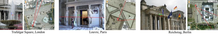
2        Yunpeng Li, Noah Snavely, Dan Huttenlocher, and Pascal Fua

Fig. 1. A worldwide point cloud database. In order to compute the pose of a query image, we
match it to a database of georeferenced structure from motion point clouds assembled from photos
of places around the world. Our database (left) includes a street view image database of downtown
San Francisco and Flickr photos of hundreds of landmarks spanning the globe; a few selected
point cloud reconstructions are shown here. We seek to compute the georeferenced pose of new
query images, such as the photo of Chicago on the right, by matching to this worldwide point
cloud. Direct feature matching is very noisy, producing many incorrect matches (shown as red
features). Hence, we devise robust new techniques for the pose estimation problem.

    Our method directly establishes correspondence between 2D features in an image
and 3D points in a very large point cloud covering many places around the world, then
computes a camera pose consistent with these feature matches. This approach follows
recent work on direct 2D-to-3D registration [8, 9], but at a dramatically larger scale—we
use a 3D point cloud created by running structure from motion (SfM) on over 2 million
images, resulting in over 800,000 reconstructed images and more than 70 million 3D
points, covering hundreds of distinct places around the globe. This dataset, illustrated
in Figure 1, is drawn from three individual datasets: a landmarks dataset created from
over 200,000 geotagged high-resolution Flickr photos of world’s top 1,000 landmarks,
the recent San Francisco dataset with over a million images covering downtown San
Francisco [7], and a smaller dataset from a university campus with accurate ground truth
query image locations [10].
    While this model only sparsely covers the Earth’s surface, it is “worldwide” in the
sense that it includes many distinct places around the globe, and is of a scale more than
an order of a magnitude beyond what has been attempted by previous 2D-to-3D pose
estimation systems (e.g., [8, 9]). At this scale, we found that noise in the feature matching
process—due to repeated features in the world and the difficulty of nearest neighbor
matching at scale—necessitated new techniques. Our main contribution is a scalable
method for accurately recovering 3D camera pose from a single photograph taken at an
unknown location, going well beyond the rough identification of position achieved by
today’s large-scale image localization methods. Our 2D-to-3D matching approach to
image localization is advantageous compared with image retrieval approaches because
the pose estimate provides a powerful geometric constraint for validating a hypothesized
location of an image, thereby improving recall and precision. Even more critically, we
can exploit powerful priors over sets of 3D points, such as their co-visibility relations,
to address both scalability and accuracy. We show state-of-the-art results compared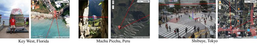
Worldwide Pose Estimation using 3D Point Clouds        3

with other localization methods, and require only a few seconds per query, even when
searching our entire worldwide database.
    A central technical challenge is that of finding good correspondences to image
features in a massive database of 3D points. We start with a standard approach of using
approximate nearest neighbors to match SIFT [11] features between an image and a set
of database features, then use a hypothesize-and-test framework to find a camera pose
and a set of inlier correspondences consistent with that pose. However, we find that with
such large 3D models the retrieved correspondences often contain so many incorrect
matches that standard matching and RANSAC techniques have difficulty finding the
correct pose. We propose two new techniques to address this issue. The first is the use of
statistical information about the co-occurrence of 3D model points in images to yield
an improved RANSAC scheme, and the second is a bidirectional matching algorithm
between 3D model points and image features.
    Our first contribution is based on the observation that 3D points produced by SfM
methods often have strong co-occurrence relationships; some visual features in the
world frequently appear together (e.g., two features seen at night in a particular place),
while others rarely appear in the same image (e.g., a daytime and nighttime feature).
We find such statistical co-occurrences by analyzing the large numbers of images in
our 3D SfM models, then use them as a new sampling prior for RANSAC in order
to efficiently find sets of matches that are likely to be geometrically consistent. This
sampling technique can often succeed with a small number of RANSAC rounds even
with inlier rates of less than 1%, which is critical for speed and accuracy in our task.
Second, we present a bidirectional matching scheme aimed at boosting the recovery of
true correspondences between image features and model points. It intelligently combines
the traditional “forward matching” from features in the image to points in the database,
with the recently proposed “inverse matching” [8] from points to image features. We
show this approach performs better than either forward or inverse matching alone.
    We present a variety of results of our method, including quantitative comparisons
with recent work on image localization [8, 7, 9] and qualitative results showing the
full, 6-degree-of-freedom (plus intrinsics) pose estimates produced by our method. Our
method yields better results than the image-retrieval-style method of Chen et al.[7] when
both use only image features, and achieves nearly the same performance—again, using
image features alone—even when their approach is provided with approximate geotags
for query images. We evaluate localization accuracy on a smaller dataset with precise
geotags, and show examples of the recovered field of view superimposed on satellite
photos for both outdoor and indoor images.

2   Related Work
Our task of worldwide pose estimation is related to several areas of recent interest in
computer vision.
Landmark recognition and localization. The problem of “where was this photo taken?”
can be answered in several ways. Some techniques approach the problem as that of classi-
fication into one of a predefined set of places (e.g., “Eiffel Tower,” “Arc de Triomphe”)—
i.e., the “landmark recognition/classification” problem [12, 13]. Other methods create a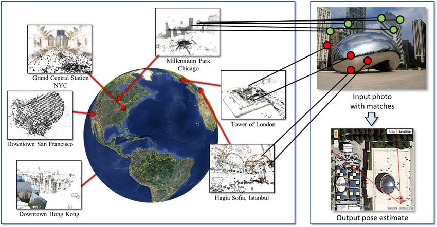
4       Yunpeng Li, Noah Snavely, Dan Huttenlocher, and Pascal Fua

database of localized imagery and formulate the problem as one of image retrieval, after
which the query image can be associated with the location of the retrieved images. For
instance, in their im2gps work, Hays and Efros seek to characterize the location of ar-
bitrary images (e.g., of forests and deserts) with a rough probability distribution over the
surface of Earth, but with coarse confidences on the order of hundreds of kilometers [4].
In follow-up work, human travel priors are used to improve performance for sequences
of images [14], but the resulting locations are still coarse. Others seek to localize urban
images more precisely, often by matching to databases of street-side imagery [6, 7, 15–
18] often using bag-of-words retrieval techniques [19, 20]. Our work differs from these
retrieval-based methods in that we seek not just a rough camera position (or distribution
over positions), but a full camera matrix, with accurate position, orientation, and focal
length. To that end, we match to a georegistered 3D point cloud and find pose with re-
spect to these points. Other work in image retrieval also uses co-occurrence information,
but in a different way from what we do. Chum et al. use co-occurrence of visual words
to improve matching [21] by identifying confusing combinations of visual words, while
we find use co-occurrence to guide sampling of good matches.
Localization from point clouds. More similar to our approach are methods that leverage
results of SfM techniques. Irschara et al. [22] use SfM reconstructions to generate a set
of “virtual” images that cover a scene, then index these as documents using BoW meth-
ods. Direct 2D-to-3D approaches have recently been used to establish correspondence
between a query image and a reconstructed 3D model, bypassing an intermediate image
retrieval step [8, 9]. While “inverse matching” from 3D points to image features [8] can
sometimes find correct matches very quickly though search prioritization, results with
this method becomes more difficult on the very large models we consider here. Similarly,
the large scale will also pose a severe challenge to the method of Sattler et al. [9] as
the matches becomes more noisy; this system already needs to perform RANSAC for
up to a minute to ensure good results on much smaller models. In contrast, our method,
aided by co-occurrence sampling and bidirectional search techniques, is able to handle
much larger scales while requiring only a few seconds per query image. Finally, our
co-occurrence sampling method is related to the view clustering approach of Lim et
al. [3], but uses much more detailed statistical information.

3   Efficient Pose Estimation
Our method takes as input a database of georegistered 3D points P resulting from
structure from motion on an set of database images D. We are also given a bipartite
graph G specifying, for each 3D point, the database images it appears in, i.e., a point
p ∈ P is connected to an image J ∈ D if p was detected and matched in image J. For
each 3D point p we denote the set of images in which p appears (i.e., its neighbors in
G) as Ap . Finally, one or more SIFT [11] descriptors is associated with each point p,
derived from the set of descriptors in the images Ap that correspond to p; in our case we
use either the centroid of these descriptors or the full set of descriptors. To simplify the
discussion we initially assume one SIFT descriptor per 3D point.
    For a query image I (with unknown location), we seek to compute the pose of
the camera in a geo-referenced coordinate system. To do so, we first extract a set of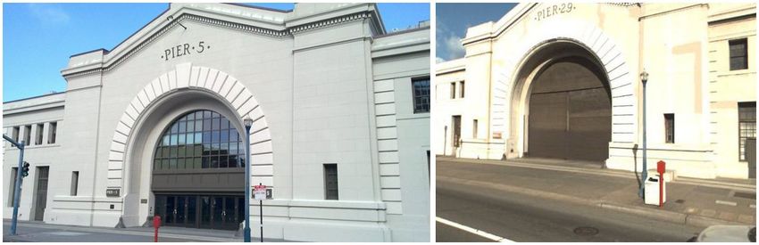
Worldwide Pose Estimation using 3D Point Clouds              5

Fig. 2. Examples of frequently co-occurring points as seen in query images. Notice that such points
are not always close to each other, in either 3D space or the 2D images.

SIFT feature locations and descriptors Q from I. To estimate the camera pose of I, a
straightforward approach is to find a set of correspondences, or matches, between the
2D image features Q and 3D points P (e.g., using approximate nearest neighbor search).
The process yields a set of matches M, where each match (q, p) ∈ M links an image
feature q ∈ Q to a 3D point p ∈ P. Because these matches are corrupted by outliers, a
pose is typically computed from M using robust techniques such as RANSAC coupled
with a minimal pose solver (e.g., the 3-point algorithm for pose with known focal length).
To reduce the number of false matches, nearest neighbor methods often employ a ratio
test that requires the distance to the nearest neighbor to be at most some fraction of the
distance to the second nearest neighbor.
    As the number of points in the database grows larger, several problems with this
approach begin to appear. First, it becomes harder to find true nearest neighbors due to the
approximate nature of high-dimensional search. Moreover, the nearest neighbor might
very well be an incorrect match (even if a true match exists in the database) due to similar-
looking visual features in different parts of the world. Even if the closest match is correct,
there may still be many other similar points, such that the distances to the two nearest
neighbors have similar values. Hence, in order to get good recall of correspondence, the
ratio test threshold must be set ever higher, resulting in poor precision (i.e., many outlier
matches). Given such noisy correspondence, RANSAC methods will need to run for
many rounds to find a consistent pose, and may fail outright. To address this problem,
we introduce two techniques that yield much more efficient and reliable pose estimates
from very noisy correspondences: a co-occurrence-based sampling prior for speeding up
RANSAC and a bidirectional matching scheme to improve the set of putative matches.

3.1   Sampling with Co-occurrence Prior

As a brief review, RANSAC operates by selecting samples from M that are minimal
subsets of matches for fitting hypothesis models (in our case, pose estimates) and then
evaluating each hypothesis by counting the number of inliers. The basic version of
RANSAC forms samples by selecting each match in M uniformly at random. There
is a history of approaches that operate by biasing the sampling process towards better
subsets. These include guided-MLESAC [23], which estimates the inlier probability
of each match based on cues such as proximity of matched features; PROSAC [24],
which samples based on a matching quality measure; and GroupSAC [25], which selects
samples using cues such as image segmentation. In our approach, we use image co-
occurrence statistics of 3D points in the database images (encoded in the bipartite graph
G) to form high-quality samples. This leads to a powerful sampling scheme: choosing
subsets of matched 3D points that we believe are likely to co-occur in new query images,
based on prior knowledge from the SfM results. In other words, if we denote with PM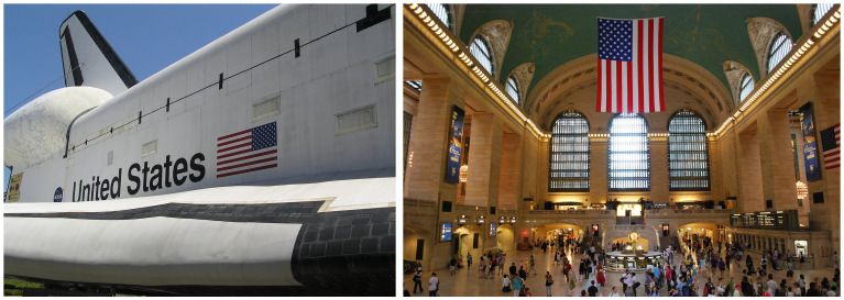
6          Yunpeng Li, Noah Snavely, Dan Huttenlocher, and Pascal Fua

the subset of 3D points involved in the set of feature matches M, then we want to
sample with higher probability subsets of PM that co-occur frequently in the database,
hence biasing the sampling towards more probable subsets. Unlike previous work, which
tends to use simple evidence from the query image, our setting allows for a much more
powerful prior due to the fact that we have multiple (for some datasets, hundreds) of
images viewing each 3D point, and can hence leverage statistics not available in other
domains. This sampling scheme enables our method to easily handle inlier rates as low
as 1%, which is essential as we use a permissive ratio test to ensure high enough recall
of true matches. Figure 2 shows some examples of frequently co-occurring points; note
that these points are not always nearby in the image or 3D space.
    Given a set of putative matches M, and a minimal number of matches K we need to
sample to fully constrain the camera pose, the goal in each round of RANSAC is to select
such a subset of matched points,1 {p1 , . . . , pK } ⊆ PM , proportional to an estimated
probability that they jointly correspond to a valid pose, i.e.,
                          Pr select (p1 , . . . , pK ) ∝ Pr valid (p1 , . . . , pK ).              (1)
As a proxy for this measure, we define the likelihood to be proportional to their empirical
co-occurrence frequency in the database, taking the view that if a set of putative points
were often seen together before, then they are likely to be good matches if seen together
in a new image. Specifically, we define:
                           Pr select (p1 , . . . , pK ) ∝ |Ap1 ∩ · · · ∩ ApK | ,                   (2)
i.e., the number of database images in which all the K points are visible. If all of the
image sets Ap1 , . . . ApK are identical and have large cardinality, then Pr select is high; if
any two are disjoint, then Pr select is 0.
     As it is quite expensive to compute and store such joint probabilities for K larger
than 1 or 2 (in our case, 3 or 4), we instead opt to draw the points sequentially, where
the i-th point is selected by marginalizing over all possible future choices:
                                                      X
                 Pr select (pi |p1 , . . . , pi−1 ) ∝   |Ap1 ∩ · · · ∩ ApK |.              (3)
                                                      pi+1 ,...,pK

In practice, the summation over future selections (pi+1 , . . . , pK ) can still be slow. To
avoid this expensive forward search, we approximate it using simply the co-occurrence
frequency of the first i points, i.e.,
                          P̃rselect (pi |p1 , . . . , pi−1 )∝ |Ap1 ∩ · · · ∩ Api | .               (4)
Given precomputed image sets Ap , this quantity can be evaluated efficiently at runtime
using fast set intersection.2
    We also tried defining Pr select using other measures, such as the Jaccard index and
the cosine similarity between Ap1 ∩ · · · ∩ Api−1 and Api , but found that using simple
co-occurrence frequency performed just as well as these more sophisticated alternatives.
 1
     Here we assume that each point p is matched to at most one feature in Q, and hence appears at
     most once in M. We find that this is almost always the case in practice.
 2
     While our method requires that subsets of three or four points often be co-visible in the database
     images, this turns out to be a very mild assumption given the further constraints we use to
     determine correct poses, described below.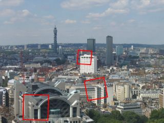
Worldwide Pose Estimation using 3D Point Clouds          7

3.2   Bidirectional Matching

The RANSAC approach described above assumes a set of putative matches; we now
return to the problem of computing such a set in the first place. Matching an image
feature to a 3D point amounts to retrieving the feature’s nearest neighbor in the 128-D
SIFT space, among the set of points P in the 3D model (using approximate nearest
neighbor techniques such as [26]), subject to a ratio test. Conversely, one could also
match in the other direction, from 3D points to features, by finding for each point in P
its nearest neighbor among image features Q, subject to the same kind of ratio test. We
call the first scheme (image feature to point) forward matching and the second (point to
feature) inverse matching. Again, we begin by assuming there is a single SIFT descriptor
associated with each point.
     We employ a new bidirectional matching scheme combining forward and inverse
matching. A key observation is that visually similar points are more common in our 3D
models than they are in a query image, simply because our models tend to have many
more points (millions) than an image has features (thousands). A prominent point visible
in a query image sometimes cannot be retrieved during forward matching, because it
is confused with other points with similar appearance. However it is often much easier
to find the correct match for such a point in the query image, where the corresponding
feature is more likely to be unique. Hence inverse matching can help recover what
forward matching has missed. On the other hand, inverse matching alone is inadequate
for large models, even with prioritization [8], due to the much higher proportion of
irrelevant points for any given query image and hence the increased difficulty in selecting
relevant ones to match. This suggests a two-step approach:

 1. Find a set of primary matches using the conventional forward matching scheme, and
    designate as preferred matches a subset of them with low distance ratios (and hence
    relatively higher confidence);
 2. Augment the set of primary matches by performing a prioritized inverse matching [8],
    starting from the preferred matches as the model points to search for in the images.
    The final pose estimation is carried out on the augmented set of matches.

We apply these two steps in a cascade: we attempt pose estimation as soon as the
primary matches are found and skip the second step if we already have enough inliers to
successfully estimate the pose.
    As mentioned above, a 3D point can have multiple descriptors since it is associated
with features from multiple database images. Hence we can choose to either compute
and store a single average descriptor for each point (as in [8, 9]) or keep all the individual
descriptors; we evaluate both options in our experiments. In the latter case, we relax the
ratio test so that, besides meeting the ratio threshold, a match is also accepted if both the
nearest neighbor and the second nearest neighbor (of the query feature) are descriptors
of the same 3D point. This is necessary to avoid “self confusion,” since descriptors for
the same point are expected to be similar. While this represents a less strict test, we
found that it works well in practice. The same relaxation also applies to the selection of
preferred matches. For inverse matching, we always use average descriptors.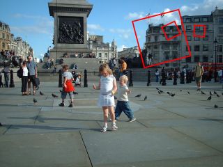
8        Yunpeng Li, Noah Snavely, Dan Huttenlocher, and Pascal Fua

Table 1. Statistics of the data sets used for evaluation, including the sizes of the reconstructed
3D models and the number of test images. SF-1 refers to the San Francisco data set with image
histogram equalization and upright SIFT features [7], while SF-0 is the one without. Note that
SF-0 and SF-1 are derived from the same image set.

             Images in      Points in Test                 Images in        Points in Test
             3D model       3D model images                3D model         3D model images
    Landmarks 205,162      38,190,865 10,000 Quad             4,830         2,022,026   348
    SF-0      610,773      30,342,328    803 Dubrovnik [8]    6,044         1,975,263   800
    SF-1      790,409      75,410,077    803 Rome [8]        15,179         4,067,119 1,000

4    Evaluation Datasets

To provide a quantitative evaluation of the localization performance of our method, we
have tested on three datasets, both separately and combined into a single point cloud;
some are from the literature to facilitate benchmarking. Table 1 summarizes each dataset.
The sizes of the Dubrovnik and Rome datasets used in [8] are included for comparison;
our combined model is about two orders of magnitude larger than the Rome dataset.
Landmarks. The first dataset consists of a large set of geotagged photos (i.e., photos with
latitude and longitude) of famous places downloaded from Flickr. We first created a list of
geotagged Flickr photos from the world’s top 1,000 landmarks derived via clustering on
geotags by Crandall et al. [27]. We ran SfM on each of these 1,000 individual collections
to create a set of point cloud models [28], estimated the upright orientation of each
model, then geo-registered the reconstructed 3D model using the image geotags, so
that its coordinates can be mapped to actual locations on the globe. Since the geotags
are quite noisy, we used RANSAC to estimate the required 2D translation, 1D rotation,
and scale. This sometimes produced inaccurate results, which could be alleviated in
the future by more robust SfM and georegistration methods [29]. Finally, we took the
union of these SfM models to form a single, geo-referenced point cloud. Some of the
individual models are illustrated in Figure 1.
     For evaluation, we created a set of test images by removing a random subset of
10,000 images from the reconstruction. This involves removing them from the image
database and their contribution to the SIFT descriptors of points, and deleting any 3D
points that are no longer visible in at least two images. Withholding the test images
slightly reduces the database size, yielding the sizes shown in Table 1. Each test image
has a known landmark ID, which can be compared with the ID inferred from an estimated
camera pose for evaluation. This ID information is somewhat noisy due to overlapping
landmarks, but can provide an upper bound on the false registration rate for the dataset.
Since the test images come from the original reconstructions, it should be possible to
achieve a 100% recall rate.
San Francisco. We also use the recently published San Francisco dataset [7], which
contains 640x480 resolution perspective images cropped from omnidirectional panora-
mas. Two types of images are provided: about 1M perspective central images (“PCIs”),
and 638K perspective frontal images (“PFIs”) of rectified facades. Each database image,
as well as each of 803 separate test images taken by cameraphones (not used in recon-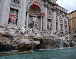
Worldwide Pose Estimation using 3D Point Clouds                              9

                                                           Registration Performance                   100
                                                                                                                Avg. descriptors
                                               100                                                              All descriptors

                Percent of Images Registered
                                                90                                                    95
                                                80
                                                70                                                    90
                                                60
                                                50
                                                                                                      85
                                                40
                                                30                        With co-occurrence, r=0.9
                                                                          W/o co-occurrence, r=0.7    80
                                                20
                                                                          W/o co-occurrence, r=0.8
                                                10                        W/o co-occurrence, r=0.9
                                                 0                                                    75
                                                     10           100          1000           10000         Forward, Forward,       Bidirect., Bidirect.,
                                                          Number of RANSAC Sampling Rounds                  no co-occ. w/ co-occ.   no co-occ. w/ co-occ.

Fig. 3. Registration rates on Landmarks. Left: comparison of results with and without co-
occurrence prior for sampling under forward matching. At 10,000 rounds, RANSAC starts to
approach the running time of the ANN-based matching. Right: comparison of forward vs. bidirec-
tional matching. We used 10,000 RANSAC rounds and selected 0.8 as the ratio threshold for the
experiments without using co-occurrence (0.9 otherwise). For comparison, applying the systems
of [8] and [9] on this same data set yielded registration rates of 33.09% and 16.20% respectively.

struction), comes with a building ID, which can be used to evaluate the performance of
image retrieval or, in our case, pose estimation. We reconstructed our 3D model using
only the PCIs (as the PFIs have non-standard imaging geometry). We reconstructed two
SfM models, one (SF-0) using the raw PCIs (to be consistent with the other datasets),
and one (SF-1) using upright SIFT features extracted from histogram-equalized versions
of the database images (as recommended in [7]). The model was georegistered using
provided geotags. We ignore images that were not reconstructed by SfM.
Quad. The first two datasets only provide coarse ground truth for locations, in the
form of landmark/building identifiers. Although geotags exist for the test images, they
typically have errors in the tens (or hundreds) of meters, and are thus too imprecise
for fine evaluation of positional accuracy. We therefore also use the Quad dataset from
Crandall et al. [10], which comes with a database of images of the Arts Quad at Cornell
University as well as a separate set of test images with accurate, sub-meter error geotags.
We ran SfM on the database images, and use the accurately geotagged photos to test
localization error.

5    Experiments and Results
To recap: to register a query image, we estimate its camera pose by extracting SIFT
features Q, finding potential matches M with the model points P through nearest
neighbor search plus a ratio test, and running co-occurrence RANSAC to compute the
pose, followed by bidirectional matching if this initially fails. For the minimal pose
solver, we use the 3-point algorithm if the focal length is approximately known, e.g.,
from EXIF data, or the 4-point algorithm [30] if the focal length is unknown and needs
to be estimated along with the extrinsics. Finally a local bundle adjustment is used to
refine the pose. We accept the pose if it has at least 12 inlier matches, as in [8, 9].
Precision and recall of registration. We first test the effectiveness of exploiting point
co-occurrence statistics in RANSAC using registration rate, i.e., the percentage of query
images registered to the 3D model. We later estimate the likelihood of false registrations.
    Figure 3 (left) shows the registration rates on the Landmarks data set. For RANSAC
with co-occurrence prior, we always use 0.9 as the ratio test threshold. For regular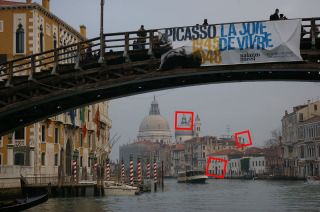
10       Yunpeng Li, Noah Snavely, Dan Huttenlocher, and Pascal Fua

Fig. 4. Estimated poses for the Landmarks dataset. A few images that were successfully regis-
tered, along with their estimate pose overlaid on a map. Each map has been annotated to indicate
the estimated position, orientation, and field of view of the photo, and the image itself is drawn
with a red line showing the horizon estimated from the pose, as well as axes showing the estimated
up (blue), north (green), and east (red) directions. (Best viewed on screen when enlarged.)

RANSAC without co-occurrence we experimented with three thresholds (r=0.7, 0.8,
0.9), the best of which at 10,000 RANSAC rounds (r=0.8) has performance roughly
equal to running just 10 rounds with co-occurrence. These results demonstrate the
advantage of using co-occurrence to guide sampling, especially when the number of
rounds is small. For this experiment, we used average SIFT descriptors for points (cf.
Sec 3). When using all of its associated descriptors for each point, we observed the same
trend as in Figure 3. The overhead incurred by co-occurrence sampling is only a small
fraction of the total RANSAC time; thus its impact on overall speed is almost negligible.
    We also assess the performance gain from bidirectional matching, the results of which
are shown in Figure 3 (right). Experiments were performed with average descriptors as
well as with all feature descriptors for the points. The results show that bidirectional
matching significantly boosts the registration rate, whether or not co-occurrence based
RANSAC is used. Similarly, the use of co-occurrence is also always beneficial, with
or without bidirectional matching, and the advantage is more pronounced when all
feature descriptors are used, as this produces more matches but also more outliers. Since
co-occurrence together with bidirectional matching produced the highest performance,
we use this combination for the remaining experiments.
    To estimate the precision of registration, namely the fraction of query images cor-
rectly registered, and equivalently the false registration rate, we consider the 1000-way
landmark classification problem. The inferred landmark ID is simply taken to be the
one with the most points registered with the image. The classification rate among the
registered images is 98.1% when using average point descriptors and 97.9% when using

Fig. 5. Examples of false registrations. Side-by-side: query image and its closest image in the
database by the number of common 3D points. Left: from Landmarks. The US flag appears both
on the space shuttle and in the Grand Central Railway Station. Right: from San Francisco. The
piers have nearly identical appearance.
Worldwide Pose Estimation using 3D Point Clouds 11
Table 2. Percentage of query images correctly localized (“recall rate”) for the San Francisco data
set. For our method, we report results with (SF-1) and without (SF-0) histogram equalization
and upright SIFT. We also experimented with both using average descriptors and keeping all
descriptors. For [7] we cite the recall rates (if provided) for the variants that use the same kind of
perspective images (PCIs) as we do.
Our method (no GPS) SF-0 SF-1 Chen et al. [7] SF-0 SF-1
Avg. descriptors 50.2 58.0 No GPS 20 41
All descriptors 54.2 62.5 With GPS - 49
all descriptors. However, we found that this does not mean that the remaining 2% of
images are all false registrations, since some of our landmarks visually overlap and
thus the classification objective is not always unambiguous. To better estimate the false
registration rate, we tested our method with a set of 1468 “negative images” that are
photos of other landmarks geographically distant from the top 1000 in our data set. Of
these, 10 images were registered (both for average/all descriptors), which corresponds
to a false registration rate of 0.68%. Figure 5 (left) shows an example false registration.
Indeed, the false registrations are almost always due to identical-looking signs and logos.
While it is difficult to quantitatively evaluate the accuracy of the full camera poses
on this dataset, we visualize a few recovered camera poses for the test set in Figure 4;
many of the poses are surprisingly visually accurate. Later, we describe the use of the
Quad dataset to quantitatively evaluate localization error.
We also test our method on the recent San Francisco data set of Chen et al. [7], and
compare with their state-of-the-art system for large-scale location recognition (based on
a bag-of-visual-word-style retrieval algorithm [31]). This is a much more challenging
benchmark: the database images have different characteristics (panorama crops) from the
test images (cell phone photos), and both have considerably lower resolution than those
in the Landmarks data set; moreover, unlike Landmarks, there is no guarantee that every
test image is recognizable given the database images. As in [7] we evaluate our method
using the recall rate, which corresponds to the percentage of correctly registered query
images. We consider a registration correct if the query image is registered to points of the
correct building ID according to the ground truth annotation. The results are summarized
in Table 2. Using the same images and features, our method outperforms that of [7] by a
large margin even when the latter uses the extra GPS information. Although a maximum
recall rate of 65% for SF-1 was reported in [7], achieving this requires the additional use
of the PFIs (on top of GPS) specific to this data set. Again, our method produces not
just a nearby landmark or building ID, but also a definitive camera pose, including its
location and orientation, as illustrated in Figure 6. This pose information could be used
for further tasks, such as annotating the image.
Fig. 6. Estimated poses for selected San Francisco query images. The annotations are the same
as in Figure 4. Our method produces reasonable poses for most of these benchmark images.12 Yunpeng Li, Noah Snavely, Dan Huttenlocher, and Pascal Fua
All the recall rates for our method correspond to false registration rates between
4.1% and 5.3%, which are comparable to the 95% precision used in [7]. As before, most
false registrations are due to logos and signs, though a few are due to highly similar
buildings (as in Figure 5, right). Sometimes correct registrations are judged as incorrect
because of missing building IDs in the ground truth, which leads to an underestimate of
both recall and precision.
Localization error. In order to evaluate the accuracy of estimated camera positions, we
tested our method on the Quad data set, which has accurately geotagged query images.
This is also a challenging data set, because of the differences in season between the
database images and the query images. Our method succeeded in registering 68.4% of the
query images using average descriptors and 73.0% using all desciptors. The localization
error has a mean of 5.5m and a median of 1.6m, with about 90% for images having errors
of under 10m and 95% under 20m. Hence despite relatively larger errors in database
image geotags used to geo-register the 3D model, our method was able to achieve good
localization accuracy comparable to that of consumer GPS.
Scalability. To further study the scalability of our method, we merged the reconstructed
3D models for our three datasets into a single large one by concatenating them together;
compared with the individual datasets, the merged set has many more things that could
potentially confuse a query image. For this test we used the San Francisco model without
histogram equalization or upright SIFT, so that all three models are reconstructed
using the same type of features and hence are more potent distractors of each other.
The combined model contains over 800K images and 70M points. We run the same
registration experiment for each of the three sets of query images on the combined model,
and compare the results with those from running on the individual models. Table 3 shows
the registration performance on the combined model for each test set under the same
criteria as on the individual models.3 The performance gap is negligible for Landmarks
and small (around 2%) for San Francisco. While the gap is somewhat larger for the Quad
images (about 7%), this is likely due to the fact that the Quad model is far smaller than
the other two, with fewer than 5K images and just over 2M points. Hence placing it into
the combined model corresponds to more than an order of magnitude increase in the
amount of irrelevant information. In this context, the decrease in registration rate for the
Quad query images can be considered quite modest. Furthermore our method maintains
essentially the same level of localization accuracy (mean=4.9m, median=1.9m) when
given the combined model. This shows the scalability of our method and its robustness
to irrelevant information.
For completeness, we also tested our method on the Dubrovnik and Rome datasets
from [8]. We achieved a registration rate of 100% on Dubrovnik and 99.7% on Rome,
using a single average descriptor per point, which compares favorably to results reported
in [8, 9] (94.1%/92.4% and 98.0%/97.7%, respectively). We also verified by swapping
the two sets that no Dubrovnik images were falsely registered to Rome and vice versa.
Our system takes on average a few seconds per query image of medium resolution (1–
2 megapixels), excluding the time to extract the SIFT keys, when running single-threaded
3
Registered Quad images are counted as correct if they were registered to the Quad part of the
combined model, which they all did.Worldwide Pose Estimation using 3D Point Clouds 13
Table 3. Recall rates (percent) on the combined model compared with those on individual models.
Combining the models has essentially no impact on the false registration rates. Average point
descriptors are used in these experiments.
Model \ Query images Landmarks San Francisco Quad
Individual 98.95 50.2 68.4
Combined 98.90 47.7 61.2
on a Intel Xeon 2.67 GHz CPU. While not real-time, this is quite fast considering the
size of the database, and could easily be parallelized.
Discussion. Most of the false registrations by our method involve some sort of signs or
logos, which tend to be feature-rich and are identical at different places. This suggests
that false registrations can be largely reduced if we can learn to recognize these types of
objects, or take into account contextual information. Our method can require a significant
amount of memory for storing descriptors, particularly when a point is assigned all of its
corresponding SIFT features. In the future, this could be improved through the use of
more compact descriptors [32], or by intelligently compressing the database.
6 Conclusion
We presented a method for camera pose estimation at a worldwide scale; for the level
of accuracy in pose we aim for, this is to our knowledge the largest such system that
exists. Our method leverages reconstructed 3D point cloud models aided by two new
techniques: co-occurrence based RANSAC and bidirectional matching, which greatly
improve its reliability and efficiency. We evaluated our method on several large data
sets and show state-of-the-art results. Moreover, comparable performance is maintained
when we combine these data sets into an even greater one, further demonstrating the
effectiveness and scalability of our method.
References
1. Takacs, G., Xiong, Y., Grzeszczuk, R., Chandrasekhar, V., chao Chen, W., Pulli, K., Gelfand,
N., Bismpigiannis, T., Girod, B.: Outdoors augmented reality on mobile phone using loxel-
based visual feature organization. In: Proc. Multimedia Information Retrieval. (2008)
2. Kopf, J., Neubert, B., Chen, B., Cohen, M.F., Cohen-Or, D., Deussen, O., Uyttendaele, M.,
Lischinski, D.: Deep photo: Model-based photograph enhancement and viewing. SIGGRAPH
Asia Conf. Proc. 27(5) (2008) 116:1–116:10
3. Lim, H., Sinha, S.N., Cohen, M.F., Uyttendaele, M.: Real-time image-based 6-dof localization
in large-scale environments. In: CVPR. (2012)
4. Hays, J., Efros, A.A.: IM2GPS: estimating geographic information from a single image. In:
CVPR. (2008)
5. Lalonde, J.F., Efros, A.A., Narasimhan, S.G.: Estimating the natural illumination conditions
from a single outdoor image. IJCV (2011)
6. Schindler, G., Brown, M., Szeliski, R.: City-scale location recognition. In: CVPR. (2007)
7. Chen, D.M., Baatz, G., Köser, K., Tsai, S.S., Vedantham, R., Pylvänäinen, T., Roimela, K.,
Chen, X., Bach, J., Pollefeys, M., Girod, B., Grzeszczuk, R.: City-scale landmark identification
on mobile devices. In: CVPR. (2011)14 Yunpeng Li, Noah Snavely, Dan Huttenlocher, and Pascal Fua
8. Li, Y., Snavely, N., Huttenlocher, D.P.: Location recognition using prioritized feature matching.
In: ECCV. (2010)
9. Sattler, T., Leibe, B., Kobbelt, L.: Fast image-based localization using direct 2D-to-3D
matching. In: ICCV. (2011)
10. Crandall, D., Owens, A., Snavely, N., Huttenlocher, D.: Discrete-continuous optimization for
large-scale structure from motion. In: CVPR. (2011)
11. Lowe, D.G.: Distinctive image features from scale-invariant keypoints. IJCV 60(2) (2004)
91–110
12. Li, Y., Crandall, D.J., Huttenlocher, D.P.: Landmark classification in large-scale image
collections. In: ICCV. (2009)
13. Zheng, Y.T., Zhao, M., Song, Y., Adam, H., Buddemeier, U., Bissacco, A., Brucher, F., Chua,
T.S., Neven, H.: Tour the world: building a web-scale landmark recognition engine. In: CVPR.
(2009)
14. Kalogerakis, E., Vesselova, O., Hays, J., Efros, A.A., Hertzmann, A.: Image sequence
geolocation with human travel priors. In: ICCV. (2009)
15. Zhang, W., Kosecka, J.: Image based localization in urban environments. In: International
Symposium on 3D Data Processing, Visualization and Transmission. (2006)
16. Knopp, J., Sivic, J., Pajdla, T.: Avoiding confusing features in place recognition. In: ECCV.
(2010)
17. Zamir, A.R., Shah, M.: Accurate image localization based on google maps street view. In:
ECCV. (2010)
18. Kroepfl, M., Wexler, Y., Ofek, E.: Efficiently locating photographs in many panoramas. In:
GIS. (2010)
19. Sivic, J., Zisserman, A.: Video Google: A text retrieval approach to object matching in video
s. In: ICCV. (2003) 1470–1477
20. Nistér, D., Stewénius, H.: Scalable recognition with a vocabulary tree. In: CVPR. (2006)
2118–2125
21. Chum, O., Matas, J.: Unsupervised discovery of co-occurrence in sparse high dimensional
data. In: CVPR. (2010)
22. Irschara, A., Zach, C., Frahm, J.M., Bischof, H.: From structure-from-motion point clouds to
fast location recognition. In: CVPR. (2009)
23. Tordoff, B., Murray, D.W.: Guided sampling and consensus for motion estimation. In: ECCV.
(2002)
24. Chum, O., Matas, J.: Matching with prosac - progressive sample consensus. In: CVPR. (2005)
220–226
25. Ni, K., Jin, H., Dellaert, F.: Groupsac: Efficient consensus in the presence of groupings. In:
ICCV. (2009)
26. Arya, S., Mount, D.M.: Approximate nearest neighbor queries in fixed dimensions. In:
ACM-SIAM Symposium on Discrete Algorithms. (1993)
27. Crandall, D., Backstrom, L., Huttenlocher, D., Kleinberg, J.: Mapping the world’s photos. In:
WWW. (2009)
28. Agarwal, S., Snavely, N., Simon, I., Seitz, S.M., Szeliski, R.: Building rome in a day. In:
ICCV. (2009)
29. Strecha, C., Pylvanainen, T., Fua, P.: Dynamic and scalable large scale image reconstruction.
In: CVPR. (2010)
30. Bujnak, M., Kukelova, Z., Pajdla, T.: A general solution to the p4p problem for camera with
unknown focal length. In: CVPR. (2008)
31. Philbin, J., Chum, O., Isard, M., Sivic, J., Zisserman, A.: Object retrieval with large vocabu-
laries and fast spatial matching. In: CVPR. (2007)
32. Strecha, C., Bronstein, A.M., Bronstein, M.M., Fua, P.: LDAHash: Improved matching with
smaller descriptors. In: EPFL-REPORT-152487. (2010)You can also read