Affection, Speed Dating and Heart Breaking - Kai A. Konrad Discussion Paper
←
→
Page content transcription
If your browser does not render page correctly, please read the page content below
Kai A. Konrad

Affection, Speed Dating
and Heart Breaking

Discussion Paper
SP II 2013–309
August 2013

Research Area
Markets and Choice
Research Unit
Economics of Change
Wissenschaftszentrum Berlin für Sozialforschung gGmbH
Reichpietschufer 50
10785 Berlin
Germany
www.wzb.eu

Copyright remains with the authors.

Discussion papers of the WZB serve to disseminate the research results of work
in progress prior to publication to encourage the exchange of ideas and aca-
demic debate. Inclusion of a paper in the discussion paper series does not con-
stitute publication and should not limit publication in any other venue. The
discussion papers published by the WZB represent the views of the respective
author(s) and not of the institute as a whole.

Affiliation of the authors:

Kai A. Konrad, Max Planck Institute for Tax Law and Public Finance, and WZB
Abstract

Affection, Speed Dating and Heart Breaking *

This paper explores the role of unilateral and idiosyncratic affection rents (’love’) from
being married with a specific individual in a matching model with individuals with heter-
ogenous matching frequencies. We show that individuals suffer in expectation from being
matched with individuals with high matching frequency. High-frequency daters have high
reservation utilities for entering into a marriage. This makes them turn down many offers
and makes them appear as ’heart-breakers’.

Dieses Paper untersucht ein Matching-Modell, in dem Heiratsentscheidungen auf der Basis
von gegenseitiger Zuneigung ("emotionalen Renten") getroffen werden. Die Rolle von Ein-
kommen und sozialem Status wird in der Analyse bewusst ausgeblendet. Es zeigt sich: Per-
sonen, die häufiger als andere Personen auf neue mögliche Partner treffen (sogenannte
"Speed Dater"), neigen dazu, auch dann weiterzusuchen, wenn die Zuneigung zu einem ge-
rade aktuellen Partner bereits sehr hoch ist. Speed Dater wirken deshalb oft als "Herzens-
brecher", obgleich ihr Verhalten nur aus ihrer Optimierungssituation entspringt, in der sie
ihre Entscheidung treffen. Die Existenz solcher "Speed Dater" verschlechtert zudem die
Situation für Personen, die eher selten auf mögliche neue Partner treffen.

Keywords: marriage, affection rent, love, matching, non-hierarchical heterogeneity

JEL classification: J12

* E-mail: kai.konrad@tax.mpg.de
I thank Salmai Qari for comments. The usual caveat applies.
1 Introduction
In this paper we analyze the role of heterogeneity in dating frequencies in a
matching framework in which emotional affection and emotional rents from
spending one’s life with one’s significant other is the main motivation for
marriage. We identify a negative externality which individuals with a high-
frequency of matching cause other individuals that results from their different
behavior in terms of their decision of whether or not to propose. Intuitively,
such high-frequency daters can afford to be picky, and will be picky in equilib-
rium due to the fact that they choose from a larger set of possible patterns in
a short amount of time. Rejecting a partner is less costly for high-frequency
daters than it is for people who only meet very few partners in the same
period of time. Therefore, they are more likely not to propose in a given
match, hence causing matches that are futile for the partners involved.
As a consequence, high-frequency daters exhibit a tendency for a particu-
lar social behavior in equilibrium. They are ’heartbreakers’ in the sense that
they are more often proposed to than they themselves propose and eventu-
ally turn down a potentially large number of offers. As male persons, they
meet one partner after the other in fairly short time intervals, only to turn
them down after meeting them. Typical labels awarded to them are those of
’womanizers’, ’playboys’ or ’Casanovas’ if they are male. Female persons who
behave similarly are given labels that receive similarly low social approval.
These labels have a connotation that hints at emotional aspects of part-
nership and at moral categories. Our matching theory can explain the ’heart
breaker’ phenomenon as well as the social disapproval of such behavior. This
theory does not resort to differences in the moral standards different indi-
viduals may have but explains the differences in behavior as an outcome of
differences in constraints, and it explains the social perspective of this phe-
nomenon as an outcome of externalities in search markets and of differences
in matching frequencies. Empirically, one should expect considerable hetero-
geneity in this frequency due to a number of reasons. Some individuals are
more afraid of being rejected when approaching a partner than others. Some
2persons may live in remote areas where they meet very few others, compared
to inhabitants of metropolitan areas.1 Job design and leisure activities also
matter. And some persons may use institutions designed to increase the
frequency by which they meet potential partners.2
The matching problem we consider is based on heterogeneity of match
quality in terms of emotional affection, or the quality of the match-specific
fit with respect to lifestyle and preferences.3 Unlike heterogeneity along an
objective, match-unspecific and vertically ordered characteristic such as in-
come or status that dominates the marriage matching literature4 , we consider
match quality of a person that is match-specific, non-transferable, and that
cannot be ordered objectively: when person A meets person B, A may feel
more or less of an affection for B, and B may feel more or less of an affection
for A. Affection need not be mutual or reciprocal, and affection is idiosyn-
cratic to the respective match. Examples of strong mutual feelings as well
as asymmetric feelings make up for a large share of romantic literature. It is
this type of non-vertical heterogeneity which we consider. More generally, we
allow for independent, unidirectional and match-specific subjective benefits
from partnership.5
1
Gautier, Svarer and Teulings (2010) take the lower search frictions in cities as the
starting point of their theoretical and empirical analysis of differences in migration patterns
between rural and urban areas for singles and for married couples.
2
Sports and dance clubs, ’speed dating services’ which provide an institutional set-up
which guarantees participants the opportunity to communicate with a certain number of
potential partners in a very short time interval and internet partnership platforms are the
most obvious and straightforward examples for this type of institution.
3
Hitsch, Hortaçsu and Ariely (2010a) analyse internet dating services and find evidence
for preferences for similarity along a number of characteristics.
4
A selection of important contributions includes Mortensen (1982), Burdett and Coles
(1997, 1999), MacNamara and Collins (1990), Bloch and Ryder (2000) and Smith (2006).
See also Hitsch, Hortaçsu and Ariely (2010b) for an empirical account.
5
To illustrate the non-vertical nature of this heterogeneity, such affection need not
be grounded in objective characteristics that are considered desirable attributes more
universally, such as wealth, social status or outstanding beauty. Edward the VIIIth, King
of Britain, for instance, is known for his deep devotion to Wallis Simpson who was clearly
3The assumption of idiosyncratic, match specific and potentially asym-
metric benefits from marriage is a significant departure from the standard
assumption of marriage matching models. Marriage matching models typi-
cally assume that individuals differ along one or several objectively ranked
dimensions - pizazz in the language of Burdett and Coles (1997). Income or
wealth are natural examples for pizazz. In these models pizazz is not a prop-
erty that is ’in the eyes’ of the matched partner and it does not change from
one match to the other; it is a generally acknowledged and match independent
invariant quality property of the individual. Such a ranking has important
implications. When persons of different pizazz level are matched, in these
models individuals like to be married with a partner with more pizazz. The
decision whether to marry is always unidirectional: the high-pizazz partner
is decisive, matching partners with less pizazz in a given match always aspire
to attain an ’upward marriage’, but the option is limited by the decision of
the partner with more pizazz. In the equilibrium the decision outcome for a
given match follows directly from the pizazz levels of the potential partners.
There is a mutual, and also social, understanding, making it easier for the
’low pizazz’ partner to understand and accept the reasons why the matched
partner is not satisfied with their pizazz. A rejected partner is not left with
a broken heart upon being rejected, not least because there exist no such
emotions in the model. Actually, being matched with a partner of much
higher pizazz or one with much lower pizazz is considered equally bad. Dis-
appointment only arises because the current match is not sufficiently similar
in pizazz.
The ’pizazz’ model is rich, has a number of surprising properties and can
explain a number of phenomena. But there is also a lot missing in such a
model: passion, marriage for love, jealousy, unfaithfulness and many other el-
ements that are important determinants in the marriage market - issues that
not of comparable social status, had been married before and can hardly be described as
extremely good-looking. Nevertheless, Edward’s utility from being together with her was
sufficiently high for him to be willing to give up his kingdom for her. And rumors are that
Wallis Simpson did not reciprocate the feelings he had for her to a similar extent.
4make for a good novel or movie. In our framework, we disregard ’pizazz’
completely, but we allow for match specific emotions such as partner spe-
cific affection, emotional attachment or love. Fernández, Guner and Knowles
(2005), Anderberg and Zhu (2010) and Konrad and Lommerud (2010) and
Hofmann and Qari (2011) have addressed this ’non-vertical’ heterogeneity in
matching market models.6 A framework that allows for idiosyncratic prefer-
ences of varying levels of intercorrelation in male-female matches and consid-
ers their implications in the context of a Gale-Shapley matching mechanism
is studied by Boudreau and Knoblauch (2010). Given the finite life-span
of individuals, the mating market has strong elements of non-stationarity,
leading to interesting dynamics by which the willingness to accept a given
match quality over time, as in Alpern and Reyniers (1999, 2005). Our analy-
sis resorts on assumptions that make the matching problem stationary, but
introduces and focuses on heterogeneity of matching frequency. Smith (2002)
studies a matching market for objects in which these objects can be traded
between different matching partners repeatedly, allowing for idiosyncratic
valuations of the objects and draws some conclusions from the analysis for a
process of entering and leaving in temporary partnerships. Similarly, Booth
and Coles (2010) consider ’romantic matching’ and focus on the incentives
for educational investment in a matching model in which these romantic rea-
sons are the driving force for marriage decisions. Our research focuses on the
impact of heterogeneity in dating frequencies for players’ reservation utilities
and their willingness to propose.
In the next section we describe the formal structure and characterize
the Markov perfect equilibrium in the matching model. In section 3 we
provide the comparative static properties of this equilibrium and interpret
these results. Section 4 concludes.
6
Huang, Jin and Xu (2012) acknowledge these dimensions and try to quantify their
importance. Hess (2004) acknowledges the role of emotional benefits (’love’) for the per-
sistence of marriage.
52 The formal framework
Consider the following standard matching framework. There is a continuum
of individuals. Each individual who is currently in this set is matched with
another individual as the outcome of a stochastic process. Suppose the two
individuals and are matched at time . At , each decides whether or not
to propose. If and mutually propose, they marry, leave the set and stay
together forever; no further decisions are to be made by them. They have a
life as a couple for an infinite time horizon, giving them a constant flow utility
() and () at each instant of time, the present value of which can be
calculated using the discount rate 0 that is assumed to be exogenous,
constant over time, and the same for all individuals. Individuals who marry
are replaced by new elements of which are clones of the individuals who
leave the set. If either or does not propose, the marriage does not take
place. In this case they stay as singles until the next marriage opportunity
with another individual comes up. We assume to be sufficiently large (or the
matching process to be appropriately designed) to rule out any subsequent
meeting of and . Until the next match, players receive a single’s flow of
utility, which is normalized to zero.
The matching takes place as a Poisson process. We do not look at the
precise microeconomic underpinnings of this process, but we allow for differ-
ences in the Poisson process for different individuals. More precisely, some
individuals are high-frequency daters. If ∆ refers to an arbitrarily small time
interval, their probability to meet at least one additional partner in this in-
terval is ∆. The other part of the population are low-frequency daters,
described by a matching probability ∆, with 0. We refer to these
types as -types and -types and use subscripts and to indicate that
variables refer to them, and we assume that a player’s type as well as the
size of the coefficients and are exogenously given. Also, individuals do
not change their type over time.
For any given match, we denote the exogenous and time invariant proba-
bility by which an -type is matched with another -type as ∈ (0 1) and
6with an -type with probability 1 − . Similarly, an -type is matched with
an -type with probability ∈ (0 1) and with an -type with probability
1 − . We do not describe the microfoundations of the matching process
underlying these probabilities.7
Consider now the decision whether to propose. When individual meets
individual , learns about the flow of affection rent would have spending
his or her life with , denoted as (). We assume that () is a random
draw from a uniform distribution with support [0 1]. Similarly, meets
and immediately learns about () ∈ [0 1]. As discussed, () may be
the result of emotional attachment, sympathy or other aspects which explain
why likes being together with . We do not assume that these benefits are
mutually symmetric. Hence, () and () from a marriage between the
two individuals and will typically be of different size. This assumption
describes that affection need not be reciprocated; the intensity by which one
person would like to be together with another person need not be symmetric
for the same couple. Also, these utility flows are match specific: affection
rents () and () from being together with can be very different for
two individuals and .
We search for stationary Markov perfect equilibrium (MPE). Decisions
are made only at those points in time when unmarried players are matched.
At those points of time the matched players must choose independently and
have two local strategies: propose, or not propose. If and only if both players
propose, they marry. Otherwise, they both stay unmarried and have to wait
for the next match with new partners before making the next decision. The
local strategy of a player when matched with player at time could be a
function of the whole history of the game up to that point and of itself, and
7
These assumptions are compatible with many possible microfoundations, as the match-
ing problem has a sufficiently large number of degrees of freedom (shares of -types and
-types, specific assumptions about correlation in the matching process). In particular,
we do not require = 1 − . For stationarity we adopt the standard assumption about
replacement of marrying individuals who leave the set . For a discussion of some of these
issues, see Burdett and Coles (1999).
7this may lead to other equilibria. We focus on Markov strategies, for which
the local strategy of a player is only a function of the state variables of the
system that are payoff relevant for the player. As the composition of and
the matching process are invariant over time, the only state variables affecting
the decisions of a player are his or her marital status (being unmarried),
the player’s own matching frequency parameter, the frequency of types, and
the players’ affection rents () and analogously for player in this match.
We can now characterize the stationary MPE that has the highest mar-
riage frequency as follows.
Proposition 1 (i) An MPE in stationary strategies exists that is character-
ized by threshold strategies as follows: In any given match between and ,
low-frequency types propose if () ≥ and high-frequency types propose
if () ≥ , with and determined by the system of equations
(1 − )2
= ( (1 − ) + (1 − )(1 − )) (1)
2
(1 − )2
= ( (1 − ) + (1 − )(1 − )). (2)
2
The solution to (1) and (2) exists, has and is unique. (ii) In the
equilibrium that is characterized by this solution, both low- and high-frequency
types have a higher expected utility from being matched with a low-frequency
type than being matched with a high-frequency type in this equilibrium.
Proof. To show (), let us assume that this equilibrium exists and is char-
acterized by threshold levels and for -types and for -types as in the
proposition: individuals propose if and only if their match-specific affection
rent is at least as high as the threshold level that applies. Let be an -
type. We need to confirm that this equilibrium behavior is optimal for ,
given that all other individuals follow this pattern. Consider individual ’s
local strategy choice: is indifferent about whether to propose if the present
value of staying unmarried in this time period, denoted as , is equal to the
expected present value of proposing. The individual prefers to propose (not
8propose) if the expected present value of proposing is higher (lower). Indiffer-
ence can be approximated, in line with standard optimization considerations
and using the assumption about uniform distribution of , by
∙ Z ¸
1 1 1
= (1 − ) + + (∆) (3)
1 + ∆ 1−
with
= ∆(1 − )( (1 − ) + (1 − )(1 − )). (4)
Here, 0 is a discount rate defined further above. The probability in
(4) is the probability by which the unmarried -type individual is matched
(at least) once in the time period ∆ with another individual in a sufficiently
suitable match; that is a match for which and are both sufficiently affected
by each other to find a marriage desirable. Consider (4) in detail: for small
∆, we can disregard the possibility of more than one match occurring in this
time interval. Accordingly, the factor ∆ approximates the probability with
which a match with some other individual occurs for an -type in that
period. With probability (1 − ) individual has sufficiently strong affection
for to propose. This is the case if () ≥ for individual . However,
this is not enough for the marriage to take place: individual must also be
willing to propose. Recall that, as is an -type, the next individual
whom is matched with is an -type with probability and an -type
with probability 1 − . Moreover, using equilibrium behavior by all other
players, the equilibrium probability that feels sufficient affection for to
propose and chooses to propose is (1 − ) if is an -type and (1 − ) if
is an -type. So, with probability , the individual marries and receives
the utility flow forever, where the expected , conditional on ≥ , is
Z 1
1+
= (5)
1− 2
This flow is converted into a present value given a discount rate by the
factor 1. Finally, the arbitrage condition uses the assumption that the
utility flow of unmarried persons is normalized to zero. It further assumes
9that the match occurred at the end of the time interval ∆, which is accounted
for by the term (∆), which is a second-order magnitude when ∆ becomes
infinitesimally short.
Marrying a person that yields a constant flow = from being married
with this person for an infinite time horizon yields a present value of ,
given that the discount rate is . To be indifferent between marrying this
person and continuing to search, the continuation value must be = .
Making use of this identity and dividing through by ∆, the condition (3) can
be rewritten as
∙ ¸
1 1 1+
= (1 − ) + + (∆) (6)
∆ 1 + ∆ ∆ ∆ 2
Here, the discount factor 1(1 + ∆) accounts for the fact that we consider
the payoff outcome that emerges during a time interval of small, but positive
length ∆, and (∆) accounts for payoff components that are of second order
and approach zero if ∆ → 0. Rearranging terms in (6) by collecting all
terms containing and (∆) on the right-hand side, inserting from (4),
simplifying and taking limits as regards ∆ → 0 yields
1
= (1 − )2 ( (1 − ) + (1 − )(1 − )) ) (7)
2
Both sides of this equation are functions of ∈ [0 1]. The left-hand side
is a linear function with positive slope 1 starting at = 0 and reaching 1
1
for = 1. The right-hand side starts at ( + (1 − )(1 − )) 2 and is
monotonically decreasing in , reaching zero for = 1. Accordingly, these
two functions cross exactly once for any given . We denote the −coordinate
of this intersection by () as in (1).
Similarly, the indifference condition for an -type individual is
1
= (1 − )2 ( (1 − ) + (1 − )(1 − )) ) (8)
2
This also defines a unique threshold level as a function of , denoted as ()
in (2).
10Overall, this defines the optimal threshold choice of a −type (−type)
as a function of (of ) as
⎧
⎪
⎨ 0 if () 0
∗
( ) = () if () ∈ [0 1] (9)
⎪
⎩
1 if () 1
and ⎧
⎪
⎨ 0 if () 0
∗
( ) = () if () ∈ [0 1] (10)
⎪
⎩
1 if () 1
This establishes a continuous self-mapping on a compact set
Φ( ) : [0 1] × [0 1] → [0 1] × [0 1] (11)
and this mapping has (at least) one fixed point ( ) by Brouwer’s fixed point
theorem.
The fixed point of Φ( ) constitutes the thresholds and in the MPE.
It is also clear from this that player of type (of type ) strictly prefers
to propose if () (if () ) and not to propose if the reverse
inequality holds strictly. This confirms that behavior described by the equi-
librium behavior is ’s optimal local reply to equilibrium behavior by all other
players and anticipated equilibrium behavior in potential future matches and
establishes that the fixed point of Φ( ) characterizes an MPE in stationary
strategies.
We next show that a solution for (1) and (2) has . A proof is by
contradiction. Suppose that, for some ( ) the condition ≥
holds. From (1) and (2) we have
(1−)2 (1 − ) + (1 − )(1 − )
=
1. (12)
(1−)2
(1 − ) + (1 − )(1 − )
Condition (12) implies that
(1 − ) + (1 − )(1 − ) (1−)2
. (13)
(1 − ) + (1 − )(1 − ) (1−)2
11For ≥ , for all possible values of and , the left-hand side is maximal
if = 1 and = 0, which reduces the left-hand side to
(1 − )
.
(1 − )
(1−)+(1− )(1−)
Replacing (1−)+(1− )(1−)
with this maximum in (12) leads to
(1−)2 (1 − ) (1−)
=
1.
(1−)2
(1 − ) (1−)
The last inequality can be transformed into . This, in turn, contradicts
the assumption ≥ , and this contradiction completes the proof of .
We turn now to uniqueness of the solution for (1) and (2). Consider the
slope of () and (). From (1) and (2) we obtain
2
() −(1 − ) (1−)
2
= 2 (14)
( (1 − ) + (1 − )(1 − )) 2(1−)
2
+ (1−)
2
+1
and
2
() − (1−)
2
= 2(1−) (1−)2
(15)
( (1 − ) + (1 − )(1 − )) 2 + (1 − ) + 1
2
The condition implies ()
∈ (−1 0) and ()
∈ (−1 0). This slope
restriction, in turn, implies that () and () can intersect only once.
Turn now to property (). Recall that in the equilibrium. Consider
an individual who is matched with an individual . Then, for () smaller
than the threshold ( or , depending on ’s type) does not propose, and the
decision of whether to propose is not decisive. But for all () exceeding
the threshold, proposes and has a rent that exceeds by some margin if
proposes. For , the probability that proposes is higher if is an
−type than if is an −type.
Proposition 1 establishes the existence of an MPE in stationary strategies
and characterizes this equilibrium. The equilibrium is of a simple nature: it is
12characterized by threshold values of affection rents for high-frequency daters
and low-frequency daters. Partners propose if their affection rent is at least
as high as a threshold that depends on the individual’s dating type, and a
marriage takes place if both partners have affection rents in this match that
are at least as high as their respective threshold rents. Conditions (1) and
(2) characterize a unique set of thresholds and provide an underpinning for
high-frequency daters to have a higher threshold than low-frequency daters.
Given these different thresholds, the probability that a low-frequency dater
is rejected by a high-frequency dater is higher than the probability that a
high-frequency dater is rejected by a low-frequency dater.
Uniqueness of a solution to (1) and (2) is an important property. It does
not imply, however, that the equilibrium described in Proposition 1 is the
only MPE. For instance, lack of coordination in the simultaneous choices of
whether to propose can support an MPE in which all players never propose.
To see this, suppose that all players assume that all other players never
propose. In this case each player who is matched with another player is
indifferent about whether to propose, and one of the optimal choices is not
to propose. These types of ’trivial’ equilibria are, however, sensitive to a
number of refinements. In what follows we therefore focus on the MPE that
is characterized in Proposition 1.
3 Comparative statics
We can now answer a number of comparative static questions for the MPE
that is described by the solution of (1) and (2). We find
Proposition 2 A player of type (of type ) benefits from an increase in
(an increase in ) and from a decrease in (a decrease in ).
Proof. The properties can be shown by analyzing the equilibrium conditions
(1) and (2). Their slopes have been characterized in part (i) in the proof of
Proposition 1. The slope restrictions of the functions () and () imply that
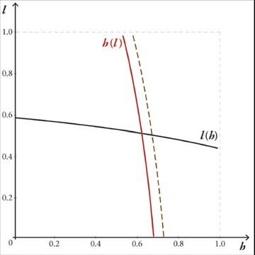
13Figure 1: The solid curves represent () and () for values = 1 = 2 and
= 12. Their slopes are in the range (0 −1), implying that they intersect only
once. The dashed line reveals how and at the intersection change if one of the
two curves shifts.
() intersects () only once, and that () intersects () from the upper
left to the lower right. The solid lines in Figure 1 illustrate these qualitative
properties and map these curves for parameter values = 1, = 2, = 12
and = 01. A change in leaves () unaffected. However, an increase
in shifts () to the upper-right. This follows from the first derivative of
(1) with respect to . This change is illustrated in Figure 1 by the dashed
line. This shift changes the point of intersection in line with Proposition 2:
the threshold is lowered and the threshold is increased. As =
and = , these thresholds are proportional to individuals’ continuation
values and . This completes the argument for an increase in . The
argument for a reduction in or a change in is fully analogous.
In conclusion, an increase in the frequency of matches for any of the two
groups increases their own reservation utility but decreases the reservation
utility of members of the respective other group. In particular, the low-
frequency daters suffer from the existence of the high-frequency daters for any
14given , as long as they may interact with them, i.e., as long as 0. The
introduction of high-frequency dating, hence, reduces match quality and life
satisfaction of those who do not want to, or cannot, participate in this dating
mechanism but still may accidentally be matched with speed daters from time
to time. This hints at an important externality of matching mechanisms that
works only for some segments of the population. It may also explain why
- given this equilibrium behavior - social prejudices and a general negative
attitude towards high-frequency daters may have developed.
We can also use the properties of the functions () and () to derive com-
parative static properties as regards the propensities by which the different
types are matched with each other. As discussed previously, the microfoun-
dation of the matching process has enough parameters (shares of −types
and -types, matching frequencies, possible positive or negative correlation
of matches of individuals of the same type) to consider variations of and
independently.
Proposition 3 A player of type (of type ) has a lower (higher) expected
payoff if is higher. A player of type (of type ) has a lower (higher)
expected payoff if is higher.
Proof. An increase in has no direct influence on (). However, for a
given , an analysis of (2) shows
(1−)2
2
( − )
= 2(1−) (1−)2
0 (16)
( (1 − ) + (1 − )(1 − )) + (1 − ) + 1
2 2
This implies that 0 induces a shift of () in Figure 1 to the left,
causing the coordinates at which () and () intersect to have a lower and
a higher .
We can make an analogous argument for an increase in . This increase
leaves () unchanged, but it shifts () inward/downward, in analogy to
(16). This leads to a new equilibrium with lower and higher .
Intuitively, recall that high-frequency daters have higher thresholds:
. If a player is matched with a high-frequency dater, the likelihood that
15this high-frequency dater does not propose to is higher than the likelihood
by which a low-frequency dater does not propose to . Accordingly, for any
given rule by which does or does not propose, the likelihood that a given
match leads to a marriage is lower if the matched person is a high-frequency
dater. For a given match frequency, it is therefore bad news for a player if
the probability for being matched with a -type is increased. Waiting for
a better match in the future becomes less attractive for an individual of
type if is higher and makes propose to less attractive matches. This,
in turn, is good news for -types, as their probability of being proposed to
in a given match goes up, and this makes them more selective. The same
logic applies for −types and an increase in their probability of being
matched with −types.
4 Discussion and conclusions
The previous sections assumed that matched partners could observe the af-
fection rent they had from being married with a matched partner at the time
when they make the marriage decision. Alternatively, they may have to base
their decision to propose on an expected value of () prior to the marriage,
rather than on a precise value. If divorce is not an option, then this does not
make a difference for the analysis.
If a divorce option comes into play, then players have the option to return
to the matching market if the marriage does not deliver a sufficient affection
rent. We would expect that some of the qualitative results about differences
between high-frequency daters and low-frequency daters can be sustained, as
the first-order effects point in a similar direction. Suppose, for instance, that
high-frequency daters’ expected equilibrium continuation payoff as unmarried
individuals is indeed higher than that of low-frequency daters. Then a divorce
and the return to the matching market is more attractive for high-frequency
daters. This, in turn, should induce them to leave a given marriage more
easily if it turns out that the true realization of () is low. If the precision
16of ’s information on () is very high at the point of marriage, divorce
is a very rare event and the results of the main section should hold true
unchanged.8
Note that these considerations about marriage with a divorce option can
also be applied to pre-marital dating behavior. If the benefit of becoming
married to a given matched partner cannot be immediately assessed in a new
match (but needs a ’trial period’ for her to find out whether the matched
male is ’Mr. Right’ and for him to find out whether the matched woman
is ’Miss Perfect’), then each match that is potentially sufficiently suitable
leads to a trial period. We can interpret a period in which two persons
were matched and had dated each other as a kind of ’trial marriage’ in
which the two persons narrow down the () and () which they would
likely have from marrying the partner they are matched with. What holds
for a real marriage with a divorce option holds similarly for such a period
of ’trial marriage’; the role of accumulated affection rents during the trial
period, however, is less pronounced than in a marriage, given that the trial
period is short. Their higher continuation value in the state in which they
are neither married nor in a ’trial marriage’ relationship is one reason why
we may expect that high-frequency daters who date a low-frequency dater
may be more likely to exit first. This behavior can contribute to the bad
reputation of high-frequency daters as emotionally instable, irresponsible or
emotionally unable to enter into a relationship. These considerations and a
formal analysis of them, however, are left for future research.
Summarizing, participants in matching markets for marriage partners are
heterogeneous along many dimensions. Much emphasis has been placed in
the past on matching markets in which individuals are sorted along a quality
8
If the precision of information on () is sufficiently low, then another effect becomes
relevant. Marriage has an option value: people may marry to find out more about their
affection rent. Within a certain range, they propose even to partners which give them an
expected affection rent that is lower than their reservation level of actual affection rent,
because of the possibility that they are positively surprised by the match in the future.
This option value is also different for daters with high and low matching frequency.
17dimension (’pizazz’) which provides an objective rank order or even a cardinal
quality scale. Here we focus on matching markets in which this hierarchical
dimension is fully absent. Potential partners are not better or worse in an
objective sense. Instead, a player has some subjective and idiosyncratic ben-
efit from marrying a particular matched partner. We called this benefit an
’affection rent’. This rent need not be mutual or symmetric. In this frame-
work matched players marry if both partners’ idiosyncratic marriage rent is
sufficiently large.
We suggest this model as a decision framework for understanding mar-
riage in matching markets because we think that it catches an important
element in marriage markets wherein some individuals unilaterally or mutu-
ally feel affection for each other, but need not have similar or even stronger
feelings of affection if meeting a more wealthy or more good-looking person.
We show that heterogeneity along this ’non-hierarchical dimension’ interacts
with heterogeneity in the probability of being matched with new partners.
We characterize a Markov perfect equilibrium in stationary strategies. The
equilibrium shows that ’high-frequency daters’ have a negative externality for
’low-frequency daters’: their higher fall-back utilities as players participating
in the matching process make them more reluctant to propose, thus, causing
them to propose less frequently. As a result, if people of different matching
frequency meet, the high-frequency dater is more likely to disappoint the
low-frequency dater.
References
[1] Alpern, Steve, and Diane Reyniers, 1999, Strategic mating with homo-
typic preferences, Journal of Theoretical Biology, 198(1), 71-88.
[2] Alpern, Steve, and Diane Reyniers, 2005, Strategic mating with common
preferences, Journal of Theoretical Biology, 237(4), 337-354.
[3] Anderberg, Dan, and Yu Zhu, 2010, The Effect of Education on Marital
Status and Partner Characteristics: Evidence from the UK, CESifo
18Working Paper No. 3104.
[4] Bloch, Francis, and Harl Ryder, 2000, Two-sided search, marriages, and
matchmakers, International Economic Review, 41(1), 93-115.
[5] Booth, Alison, and Melvyn Coles, 2010, Education, matching, and the
allocative value of romance, Journal of the European Economic As-
sociation, 8(4), 744-775.
[6] Boudreau, James W., and Vicky Knoblauch, 2010, Marriage matching
and intercorrelation of preferences, Journal of Public Economic The-
ory, 12(3), 587-602.
[7] Burdett, Kenneth, and Melvyn G. Coles, 1997, Marriage and class,
Quarterly Journal of Economics, 112(1), 141-168.
[8] Burdett, Kenneth, and Melvyn G. Coles, 1999, Long-term partner-
ship formation: marriage and employment, The Economic Journal,
109(456), 307-334.
[9] Fernández, Raquel, Nezih Guner, and John Knowles, 2005, Love and
money: a theoretical and empirical analysis of household sorting and
inequality, Quarterly Journal of Economics, 120(1), 273-344.
[10] Gautier, Pieter A., Michael Svarer, and Coen N. Teulings, 2010, Mar-
riage and the city: search frictions and sorting of singles, Journal of
Urban Economics, 67, 206-218.
[11] Hess, Gregory D., 2004, Marriage and consumption insurance: what’s
love got to do with it? Journal of Political Economy, 112(2), 290-
318.
[12] Hitsch, Günter J., Ali Hortaçsu, and Dan Ariely, 2010a, What makes
you click? - Mate preferences in online dating, QME Quantitative
Marketing and Economics, 8(4), 393-427.
[13] Hitsch, Günter J., Ali Hortaçsu, and Dan Ariely, 2010b, Matching and
sorting in online dating, American Economic Review, 100(1), 130-
163.
19[14] Hofmann, Dirk, and Salmai Qari, 2011, The Law of Attraction — Bilat-
eral Search and Horizontal Heterogeneity, Working Paper, Sonder-
forschungsbereich 649: Ökonomisches Risiko 17 (SFB 649 Papers).
[15] Huang, Fali, Ginger Zhe Jin, and Lixin Colin Xu, 2012, Love and money
by parental matchmaking: evidence from urban couples in China,
American Economic Review: Papers & Proceedings, 102(3), 555-560.
[16] Konrad, Kai A., and Kjell Erik Lommerud, 2010, Love and taxes - and
matching institutions, Canadian Journal of Economics, 43(3), 919-
940.
[17] McNamara, John M., and E. J. Collins, 1990, The job search problem as
an employer-candidate game, Journal of Applied Probability, 27(4),
815-827.
[18] Mortensen, Dale T., 1982, Property rights and efficiency in mating, rac-
ing, and related games, American Economic Review, 72(5), 968-979.
[19] Smith, Lones, 2002, A model of exchange where beauty is in the eye of
the beholder, unpublished manuscript, University of Michigan.
[20] Smith, Lones, 2006, The marriage model with search frictions, Journal
of Political Economy, 114(6), 1124-1144.
20Discussion Papers of the Research Area Markets and Choice 2013 Research Unit: Market Behavior Nadja Dwenger, Dorothea Kübler, Georg Weizsäcker SP II 2013-201 Preference for Randomization: Empirical and Experimental Evidence Kai A. Konrad, Thomas R. Cusack SP II 2013-202 Hanging Together or Being Hung Separately: The Strategic Power of Coalitions where Bargaining Occurs with Incomplete Information David Danz, Frank Hüber, Dorothea Kübler, Lydia Mechtenberg, SP II 2013-203 Julia Schmid ‘I’ll do it by myself as I knew it all along’: On the failure of hindsight- biased principals to delegate optimally David Hugh-Jones, Morimitsu Kurino, Christoph Vanberg SP II 2013-204 An Experimental Study on the Incentives of the Probabilistic Serial Mechanism Yan Chen, Onur Kesten SP II 2013-205 From Boston to Chinese Parallel to Deferred Acceptance: Theory and Experiments on a Family of School Choice Mechanisms Thomas de Haan, Roel van Veldhuizen SP II 2013-206 Willpower Depletion and Framing Effects Dietmar Fehr, Steffen Huck SP II 2013-306 Who knows it is a game? On rule understanding, strategic awareness and cognitive ability Christine Binzel, Dietmar Fehr SP II 2013-207 Giving and sorting among friends: evidence from a lab-in-the field experiment Research Unit: Economics of Change Luisa Herbst, Kai A. Konrad, Florian Morath SP II 2013-301 Endogenous Group Formation in Experimental Contests Kai A. Konrad, Florian Morath SP II 2013-302 Evolutionary Determinants of War Armin Falk, Nora Szech SP II 2013-303 Organizations, Diffused Pivotality and Immoral Outcomes Maja Adena, Steffen Huck, Imran Rasul SP II 2013-304 Charitable Giving and Nonbinding Contribution-Level Suggestions. Evidence from a Field Experiment All discussion papers are downloadable: http://www.wzb.eu/en/publications/discussion-papers/markets-and-choice
Dominik Rothenhäusler, Nikolaus Schweizer, Nora Szech                      SP II 2013-305
Institutions, Shared Guilt, and
Moral Transgression

Dietmar Fehr, Steffen Huck                                                 SP II 2013-306
Who knows it is a game? On rule understanding, strategic awareness
and cognitive ability

Maja Adena, Michal Myck                                                    SP II 2013-307
Poverty and Transitions in Health

Friedel Bolle, Jano Costard                                                SP II 2013-308
Who Shows Solidarity with the Irresponsible?

Kai A. Konrad                                                              SP II 2013-309
Affection, Speed Dating and Heart Breaking

WZB Junior Research Group: Risk and Development

Lubomír Cingl, Peter Martinsson, Hrvoje Stojic, Ferdinand M. Vieider       SP II 2013-401
Separating attitudes towards money from attitudes towards probabilities:
stake effects and ambiguity as a test for prospect theory

All discussion papers are downloadable:
http://www.wzb.eu/en/publications/discussion-papers/markets-and-choice
Bei Ihren Bestellungen von WZB-Papers schicken                      Please send a self addressed label and postage
Sie bitte unbedingt einen an Sie adressierten Auf-                  stamps in the amount of 0,55 Euro or one "Coupon-
kleber mit sowie je paper eine Briefmarke im Wert                   Réponse International" (if you are ordering from
von 0,55 Euro oder einen "Coupon Réponse Inter-                     outside Germany) for each WZB-paper requested
national " (für Besteller aus dem Ausland)

Bestellschein                                                                                      Order Form

                                                        Absender / Return Address:

Wissenschaftszentrum Berlin
für Sozialforschung
Presse- und Informationsreferat
Reichpietschufer 50

D-10785 Berlin-Tiergarten

Hiermit bestelle ich folgende(s)                     Please send me the following
Discussion paper(s):                                 Discussion paper(s):

Bestell-Nr. / Order no.                              Autor/in, Kurztitel / Author(s) / Title(s) in brief
You can also read