On the Use of Bright Scatterers for Monitoring Doppler, Dual-Polarization Weather Radars - MDPI
←
→
Page content transcription
If your browser does not render page correctly, please read the page content below
remote sensing
Technical Note
On the Use of Bright Scatterers for Monitoring
Doppler, Dual-Polarization Weather Radars
Marco Gabella       ID

 MeteoSwiss, via ai Monti 146, CH-6605 Locarno-Monti, Switzerland; marco.gabella@meteoswiss.ch;
 Tel.: +41-58-460-9692

 Received: 1 May 2018; Accepted: 21 June 2018; Published: 25 June 2018

 Abstract: “Bright” scatterers are useful for monitoring modern weather radars. In order to be “bright”,
 a point target with deterministic backscattering properties should be present at a near range and be
 hit by the antenna beam axis. In this note, a statistical characterization of the echoes from a metallic
 tower located on Cimetta, at an 18 km range and at the same altitude as the Monte Lema radar, is
 presented. The analysis is based on five clear sky days (1440 samples with a spatial resolution of
 1◦ × 1◦ × 83.33 m). The spectral and polarimetric signatures are striking: The spectrum width is
 perfectly stable; the mean radial velocity is very stable; the radar reflectivity is also quite stable, with
 the vertical (V) polarization being more variable than the horizontal (H) one. As far as the polarimetric
 information is concerned, the daily average of the differential reflectivity is approximately 1 ± 0.9 dB.
 The copolar correlation coefficient between H and V is remarkably large (0.9962, on average) and
 stable. It is believed that these unique and stable ground clutter signals could be used to monitor
 operational dual-polarization weather radars.

 Keywords: monitoring; quality checks; relative calibration; dual-polarization weather radar

1. Introduction
      Ground echo is a challenge for operational weather radars, especially as far as hydrological
applications and precipitation estimates are concerned. The identification and elimination of ground
clutter is a prerequisite for the use of weather radar. Since European radars are often used for
the surveillance of complex-orography regions, they are installed out of necessity on the top of a
hill or a mountain, where the rejection of clutter is of vital importance, since a clear view from a
high site implies a large number of ground clutter pixels. Ground clutter is automatically detected
in the operational radar processing chain of meteorological services using certain specific and
well-consolidated algorithms and then rejected so that only the radar echoes originating from the
weather are retained. In this context, the use of high range resolution (for example, cτ/2 < 100 m,
where τ is the pulse length), Doppler velocity and dual-polarization information maximizes the
probability of having at least some clutter-free radar bins for each Cartesian pixel of the resampled
operational product. The distribution of ground clutter echoes can often be fitted using one of the
following distributions: Rayleigh (independent randomly distributed scatterers, e.g., [1]), lognormal
(e.g., [2]) and Weibull (e.g., [3]). It has been found that, for these skewed-to-the-right distributions, the
Log-transformed ratio between the 90th percentile and the algebraic average of the radar reflectivity
value generally ranges between 3 and 4 dB for most ground clutter radar bin cases. Furthermore, in the
case of randomly distributed scatterers, the Log-transformed ratio between the algebraic average and
the median is 1.6 dB.
      Ground-clutter characteristics, as well as their modeling and simulation have been studied
extensively, primarily to improve the radar detection of meteorological targets (e.g., [4]). Thanks
to the increase in knowledge, together with the exponential increase in computational power for

Remote Sens. 2018, 10, 1007; doi:10.3390/rs10071007                      www.mdpi.com/journal/remotesensing
Remote Sens. 2018, 10, 1007 2 of 14
modeling and statistical analysis, a novel point of view regarding ground clutter is emerging; it is no
longer considered just a disturbance that needs to be rejected and its spatio-temporal characteristics
are instead being investigated so that they can be used to monitor the quality of radar hardware.
Silberstein et al. [5], for instance, proposed a statistical method, based on the probability distribution
of a clutter area close to a ground-based radar, to provide near-real-time estimates of the relative
calibration of reflectivity data. The original application was to an S-band radar in a tropical oceanic
location; later, Bertoldo et al. [6] successfully applied a similar approach to an X-band radar in the
more complex terrain of the Western Alps. The study by Wolff et al. [7] has shown that the technique is
capable of monitoring the reflectivity calibration of other S-band radars, given the proper generation of
an areal clutter map. The operational implementation of such techniques obviously takes into account
the reflectivity values of all the ground clutter low range resolution radar bins (generally, 1◦ × 500 m)
that are above a given high reflectivity threshold (e.g., 55 dBZ) for more than a given percentage of
time. It does not consider any other important spectral or polarimetric information that characterizes
the ground clutter bins, or perform a temporal analysis of any individual radar bins, even though these
could provide useful information for the monitoring of the quality of modern dual-polarization radars.
A guiding principle for a comprehensive radar monitoring is in fact to combine as many independent
sources of information as possible. These include: Test signals inserted at various points of the radar
chains by laboratory test equipment during preventive maintenance; signals transmitted by the radar
and measured by an external receiver to check the amplitude and shape of the transmitted radar
pulse (e.g., [8]), signals from the Sun during operational weather scanning for the daily monitoring
of the pointing accuracy of the antenna [9] and of the relative calibration of the receiver [10–12];
signals from the Sun with maximized Signal-to-Noise ratios (offline Sun-tracking on demand) for the
absolute calibration of the receiver [13]; ground clutter maps in clear sky conditions (for instance,
percentile maps).
In this technical note, we propose complementing the above-mentioned multi-sensor and
multi-signal monitoring approach with a wealth of spectral and polarimetric information associated
with an individual scatterer that we have defined as a “Bright Scatterer” (BS). In order to be “bright”,
a dominant point target, with deterministic backscattering properties, should be present in the radar bin,
which has to be located close to the radar and hit by the antenna beam axis. The particular Doppler and
polarimetric signatures of the BS emerge in one single, high-range-resolution radar bin: In the case of
the Swiss radar, the sampling volume, which depends on the antenna Half Power Beam Width (HPBW)
and the pulse length, is 1◦ × 1◦ × 83.33 m. Hence, we present detailed information regarding the bin
that contains the BS, which is a high metallic tower that has a huge radar cross section (RCS). It is located
on Cimetta at an altitude of 1650 m and has an 18 km range: the corresponding (HPBW) azimuthal
(and elevation) angular resolution is 314 m. The idea of using return signals from a radio tower is not
new. In Reference [14], for instance, the focus was on the stability of the radar reflectivity, while in
Reference [15] it was on the differential reflectivity. In this note, several other features are analyzed
in detail: the mean radial velocity and the spectrum width which complement radar reflectivity.
As far as polarimetric information is concerned, in addition to differential reflectivity, the co-polar
correlation coefficient and the differential phase shift are presented. A geographic description of the
BS location and the radar site is given in Section 2, together with detailed information regarding the
radar hardware and scan program. Section 3 presents and describes the results, which are based on the
analysis of five clear sky days (1440 samples acquired with a 5-min sampling time): It is shown that the
spectral and polarimetric signatures of the BS are impressive, in terms of stability and reproducibility.
The findings and their implications are discussed in Section 4, which also presents future research
directions. The conclusions are presented in Section 5.Remote Sens. 2018, 10, 1007 3 of 14
2. Materials and Methods
2.1. The Dual-Polarization, Doppler Radar Located on Monte Lema at an Altitude of 1625 m
In 2011, MeteoSwiss started the renewal of its weather radar network, which now consists of
five identical, dual-polarization, Doppler, C-band (5.5 GHz) radars [16]. One of them is the Monte
Lema radar, which is located at an altitude of 1625 m 10 km northwest of Lugano, very close to the
Swiss-Italian border. This is the radar that is dealt with in this study.
Radar hardware monitoring is run continuously: many parameters are monitored and submitted
from each radar site to the central server after completion of every single sweep, that is, 20 times in
5 min. These parameters are automatically checked for anomalies and archived for diagnostic analyses.
Daily monitoring of the antenna pointing accuracy [9] and of the relative calibration of the receiver has
been implemented [11], according to the Dutch/Finnish operational monitoring approach [10,12].
In order to guarantee system stability and reproducibility, instrumental calibration of the radar
receiver should be implemented using internal microwave equipment. This is performed at MeteoSwiss
using a noise source signal [17], which is inserted every 2.5 min in both polarization channels of the
receiver path, both before the T/R limiter and at the entrance of the low noise amplifiers.
The MeteoSwiss state-of-the-art C-band radars determine the standard dual-polarization
meteorological quantities (differential reflectivity, Zdr , see Section 2.2.4; copolar correlation coefficient,
ρHV , see Section 2.2.5; differential phase shift, ψdp, see Section 2.2.6) from simultaneous horizontal (H)
and vertical (V) transmissions. The return signals are measured simultaneously in two parallel H and
V receiving channels. The advantage of simultaneously transmitting and receiving both polarizations
is that Zdr , ρHV , and ψdp are determined directly from the same transmitted pulse (which is at zero
lag), and are thus not contaminated by Doppler effects that can increase their variance, as is the case
when alternating H and V polarizations are transmitted. The approach has the additional advantage
of not needing a high-power polarization switch. According to measurements performed at the Site
Acceptance Tests (i.e., twisting the transmitter or receiver horns of the Radar Target Simulator to the
following four configurations: 0◦ , 90◦ and ±45◦ ), it was possible to verify that the Lema radar is
quasi-linear and has a slant of +45◦ .
2.1.1. The Scan Program with Reference to the Target under Investigation
Each MeteoSwiss radar performs plan position indicator scans at 20 elevations, that is, from −0.2◦
to 40◦ , over a period of 5 min. Figure 2 in Reference [16] (p. 45) shows the Swiss scan strategy: It starts
with sweep #1 at an elevation of 6.5◦ and ends with sweep #20 at 9.5◦ (the first two numbers in the
figure). The 3rd and 4th numbers represent the number of antenna rotations per minute and the pulse
repetition frequency, respectively, which are relevant for the 1◦ angular bin that contains the BS at the
lowest angle of elevation. Since the PRF at this angle of elevation is 600 Hz, while the antenna takes
20 s to compute a 360◦ rotation, the BS is illuminated by a rotating antenna for 1/18 s. This means that
each high-range resolution BS “echo” (observed every 5 min and referring to the same 1◦ azimuthal
index) is the result of the spectral analysis of 600/18 ∼
= 33 pulses, when azimuthal index 349 is used.
2.2. Physical Radar Observables (and Their Quantization) Coded in High Range Resolution (83.33 m)
Radar Bins
As previously stated, the 1◦ radar bin (azimuth-range cell for a given angle of elevation) has
a high resolution range (83.33 m); its spectral and polarimetric characteristics are quantized using
1 byte, except for the differential phase shift, which is quantized with 2 bytes (namely 65,536 values).
Hence, the Digital Number (DN) can vary in binary format from 0 to 255 (65,535 in the case of the
differential phase shift). In the case of the MeteoSwiss high range resolution data, DN = 0 has no
quantitative meaning and instead has a qualitative meaning. In fact, if the Log-transformed ratio
between the Signal plus the (unknown) Noise and the (estimated) Noise is smaller than 4 dB, then the
echo is considered to be below the Minimum Detectable Signal (MDS). The corresponding radar bin isRemote Sens. 2018, 10, 1007 4 of 14
assumed to be WITHOUT (detectable) precipitation, and its DN is set to 0. More details regarding the
physical meaning of the moments used in this study (as well as their quantization) can be found in the
following six Subsections.
2.2.1. Horizontal (H) and Vertical (V) Radar Reflectivity (0th Doppler Moment)
As mentioned in Section 2.2, a high-range-resolution reflectivity value is coded as long as
S + Nu
10 Log ≥ 4 dB, (1)
Ne
where the numerator represents the power (I2 + Q2 ) of the Signal plus the (unknown) Noise of the
current bin, and the denominator is an estimate (performed every 2.5 min) of the Noise performed at
high Elevation angles (40◦ and 35◦ , see Figure 2 in Reference [16]). In other words, the measured power
(Signal plus the unknown Noise) will be at least 2.512 times the estimated Noise that will be recorded
as a quantitative value. If not, the radar bin is assumed to be without any (detectable) precipitation
and DN is set to 0 (flag value). Let us suppose that the estimate of the Noise is close to the actually
measured value: this means that the net Signal should be at least 1.512 times the Noise. As far as
quantization is concerned, a value of 0.5 dBZ has been chosen by MeteoSwiss. The linear conversion
from DN to Log-transformed radar reflectivity is the following
ZdBZ = (DN − 64)/2, (2)
where the radar reflectivity units, Z, are [Z] = mm6 /m3 , while Z1 (Z1 = 1 mm6 /m3 ) is the normalization
factor necessary to Log-transform Z into the so-called dBZ unit, which, in formula form, is:
Z
ZdBZ = 10 Log . (3)
Z1
In practice, the maximum recorded value for the Monte Lema radar very rarely exceeds 85 dBZ
(DN = 234), while DN = 14 (−25 dBZ) can, in principle, only be observed within a range of 3 km or
closer (already at the edge of the T-R limiter effects).
2.2.2. Mean Radial Velocity (1st Doppler Moment)
Since the radar wavelength is 55 mm and the PRF of the lowest elevation is 600 Hz,
the unambiguous Doppler velocity (±Nyquist) is ±8.25 m/s. As previously stated, only 255
quantitative values are used in the quantization process: this corresponds to a quantization of 0.061 m/s.
The conversion from DN to the mean radial velocity, VEL, is
VEL = (DN − 128)/127·Nyquist; (4)
Hence, DN = 1 (255) corresponds to a mean radial velocity of −8.25 (+8.25) m/s (DN = 0 is not
used). It is worth noting that the minus sign in the MeteoSwiss radar network corresponds to an
approaching target (although an approaching target is generally associated with a positive velocity).
2.2.3. Doppler Spectrum Width (2nd Doppler Moment)
As far as the spectrum width is concerned, the quantization is also 0.061 m/s
2.2.4. Differential (Horizontal/Vertical) Radar Reflectivity
A first polarimetric observable that can be measured by the MeteoSwiss dual-polarization radar is
the differential radar reflectivity, Zdr . This is the Log-transformed ratio between the copolar reflectivityRemote Sens. 2018, 10, 1007 5 of 14
measured at the horizontal, ZH, and vertical, ZV, polarizations; hence, it is expressed in dB, and a Zdr
of 0 dB means that ZH = ZV. In formula form:
ZH
Z dr = 10 Log . (5)
ZV
This ratio was introduced by Seliga and Bringi [18] to obtain a better estimate of rainfall, since
it contributes to reducing the uncertainty associated with rain drop size distributions. In fact, the
additional information associated with Zdr is remarkable; however, a proper calibration is crucial
for successful quantitative applications. Illingworth [19], for instance, showed that Zdr should be
estimated within 0.2 dB to obtain improved rainfall estimates based on Z and Zdr . It is possible to
use the so-called birdbath scan (angle of elevation of 90◦ ) on rainy days when the altitude of the 0◦
isotherm is high enough to be outside the range that is affected negatively by the T-R limiter recovery
time to monitor the differential reflectivity backscattered by liquid drops (Zdr should be 0 dB). Another
(more uncertain approach) is to derive the mean differential reflectivity value of light rain echoes (for
example, 20 ≤ ZH ≤ 22 dBZ) well below the bright band (which should be around 0.3 dB).
Offline Sun observations acquired while tracking the Sun [20,21] are more accurate, but only
the receiving chain is monitored, and nothing is therefore known regarding the transmitting path.
It is shown in Table 3 (4) in Reference [13] that the standard deviation of six (seven) Sun tracking
observations (performed between 2 November 2013 and 21 March 2016) for the MeteoSwiss Monte
Lema (Albis) radar is 0.08 (0.04) dB. An interesting and valid alternative to offline Sun-tracking is the
automatic daily “Sun-check” [10]: this is an operational monitoring technique that is based on the
analysis of solar signals in the polar volume radar reflectivity data produced during the operational
weather scan program. It has the advantage of the weather radar scan program not being interrupted;
the disadvantage is that the antenna beam axis very rarely hits the center of the Sun: consequently,
the Sun-to-Noise ratio of each hit can be significantly worse than for Sun tracking. This is partly
compensated for by the fact that only one estimate out of many daily hits is retrieved. In Reference [11]
(Table 4), the standard deviation of the daily differential reflectivity during an active solar period in
2014 was 0.06 dB for Monte Lema (220 days) and 0.05 dB for the Albis radar (204 days); the dispersion
of the difference between H and V during the same set of 100 days in 2014 was 0.06 dB for Albis and
0.08 dB for the Finish ANJ radar (see Table 3 in Reference [22]). In a recent manuscript that reviews
several aspects of the monitoring of dual-polarization receiver using solar hits found in operational
scans [12], a dispersion as low as 0.02 dB was found for ANJ. These figures refer to a shorter period,
namely April 2015. If the antenna is not in an environment with small changes in Temperature,
then differential reflectivity can easily vary by a few tens of dB [23]: in Figures 4 and 5, page 1890,
in Reference [23], it is shown that a 23 K change in temperature (lasting 8 h) occurred at the S-band
Firestone site (on 15 January 2015) and a 0.2 dB drift in Zdr was observed.
Regarding the quantization process, it is worth noting that differential reflectivity is only defined
on condition the inequality in (1) is satisfied for both the H and V polarizations. If not, DN is set to 0.
The number of radar bins that contain a valid value of differential reflectivity is obviously smaller than
for the H or V reflectivity (however, it could be at least the same). In the quantization process based on
255 values the resolution is 15.751/255 ∼ = 0.062 dB.
All the values outside the above-defined range of 15.751 dB are left- or right-saturated. Since
ZVdBZ is also saved in the MeteoSwiss archive (in addition to Zdr and ZdBZ ), the user can retrieve
the original, non-saturated value by simply subtracting ZVdBZ from ZHdBZ ; obviously, in this case,
the derived value only has a resolution of 0.5 dB, as can be seen from Equation (2).
2.2.5. The Copolar Correlation Coefficient
Another quantity measured by the dual-polarization radar is the correlation between the copolar
horizontal, HH, and the vertical, VV, returns, which is called the copolar correlation coefficient
(often referred to as ρHV or ρco ). However, describing the rather complicated nature of this variableRemote Sens. 2018, 10, 1007 6 of 14
is beyond the scope of this note. On the one hand, any reader that is interested may refer to the
electronic supplement (e06.1) that accompanies the book by Fabry [24]; on the other hand, the detailed
treatment of the physics and use of polarimetric quantities has been the subject of entire books,
e.g., Bringi e Chandrasekar [25]. The copolar correlation coefficient is the module of the complex
correlation coefficient between two orthogonal components (represented by two complex numbers)
of the backscattered electromagnetic field within the radar sampling volume: hence, it ranges from 0
(no correlation between the two polarizations) to 1 (perfect correlation). In general, if the sampling
volume contains a significant number of ground targets, then, in most cases, ρHV ranges from 0.75
to 0.95, for example. However, for the bright scatterer in Cimetta that will deal with in the Section 3,
the median of the five daily values is as large as 0.9972. A maximum value of 0.9998 has been observed.
Regarding the 1-byte quantization, a considerable resolution is attributed (through a logarithmic
transformation) to values of ρHV close to 1; hence, low values of ρHV are compressed into a few Digital
Numbers. The corresponding conversion formula from DN to ρHV is:
DN −1
ρHV = 1.003 − 10− 100 . (6)
DN = 0 corresponds to ρHV = 0, while DN = 255 is obviously not possible.
2.2.6. The Differential Phase Shift between the Two Orthogonal Polarizations
A third polarimetric quantity measured by the MeteoSwiss radars is the differential phase shift,
Ψdp , between the phase of the copolar signal at the horizontal and vertical polarizations, respectively.
This difference between the two orthogonal polarization phases arises from two sources:
• a difference in the delay introduced by the scattering of the transmitted wave, which is known as
the backscattering phase delay, δco ;
• a difference in the forward propagation velocity of the two polarizations, which is known as the
differential propagation phase, Φdp .
In formula form, the differential phase shift, Ψdp , at any given range, is:
Ψdp = δco + Φdp + Ψ0 , (7)
which is the sum of the backscattering phase delay of the targets at that range; the two-way differential
propagation phase that occurred when propagating from the radar to the observed target and then back
to the radar; an offset value Ψ0 , which is the phase difference between the transmitted and received
vertically and horizontally polarized waves at the zero range. This constant value depends on the
hardware components and design of the radar; at MeteoSwiss, this value was set close to 0◦ through a
post-facto software adjustment (and it is monitored to ensure it remains constant).
As stated in Section 2.2, the differential phase shift is the only radar observable that is quantized
using two bytes. The DN in binary form ranges from 1 to 65,535; DN = 0 is not used. The conversion
formula from DN to the value of Ψdp , which is expressed in degrees, is:
Ψdp = (DN − 32768)/32767 × 180◦ . (8)
2.3. The Metallic Tower on Cimetta at an Altitude of 1633 m: A Particularly Bright Target!
As stated in the introduction, at the Cimetta range (~18.14 km, at the center of the radar bin),
the radar resolution cell is 83.33 mm along-range and 314 m across-range (elevation and azimuth).
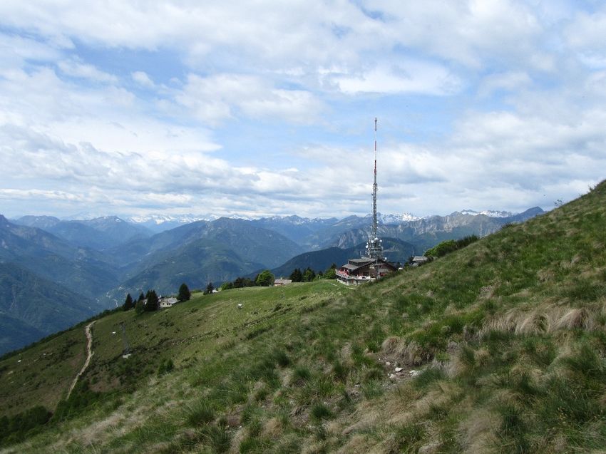
The picture in Figure 1 shows the mountainous backscattering environment that characterizes the
radar bin analyzed in this study. The view is from East to West (an azimuth of ~260◦ ) so that it is
practically orthogonal to the direction of the incident electromagnetic radar ray (the Azimuth of the
radar bin at hand is 349◦ ), which, consequently, comes from the left side of the picture. The trees onRemote Sens. 2018, 10, 1007 7 of 14
mountain were chopped down centuries ago, so that the land is basically used for grazing, with just
a few sparse trees remaining. There are some small summer cottages inside the bin, plus a (larger)
hut that is located at 30 m from the tower (East direction). The tall metallic tower is by far the largest
scatterer in the radar bin; it is orthogonal to the incident electromagnetic energy (angle of Elevation of
−0.2◦ ). It is as large as 12 × 12 m at the base and is covered by solar panels (not visible in the picture,
since they are behind the hut). There are all sorts of telecommunication and broadcasting antennas at
heights of between 6 and 12m, and then the tower becomes more slender and reaches a height of 90 m
above the ground (~1633 m altitude). This point target exhibits a very large radar cross section and
acts asSens.
Remote a dominant target
2018, 10, x FOR in aREVIEW
PEER background of randomly distributed scatterers. 7 of 14
Figure 1. Morphology of the mountainous Cimetta backscattering radar bin: small cottages, the hut,
Figure 1. Morphology of the mountainous Cimetta backscattering radar bin: small cottages, the hut,
the chairlift and the 90 m tall metallic tower.
the chairlift and the 90 m tall metallic tower.
3. Results
3. Results
The present section is aimed at providing a concise description of the experimental results and
The present section is aimed at providing a concise description of the experimental results and
their interpretation. It is divided into six subheadings that correspond to the six radar observables
their interpretation. It is divided into six subheadings that correspond to the six radar observables
introduced in Section 2.2, that is, the 2nd and the 1st Doppler moments of the horizontal polarization,
introduced in Section 2.2, that is, the 2nd and the 1st Doppler moments of the horizontal polarization,
backscattered power of both orthogonal polarizations, followed by three polarimetric quantities
backscattered power of both orthogonal polarizations, followed by three polarimetric quantities
(differential reflectivity, copolar correlation coefficient and differential phase shift). As stated in the
(differential reflectivity, copolar correlation coefficient and differential phase shift). As stated in the
introduction, when the 5-min power returns are analyzed, a random scattering pattern can be
introduction, when the 5-min power returns are analyzed, a random scattering pattern can be expected
expected that is characterized by rapid short-term fluctuations; the phase (2nd and the 1st Doppler
that is characterized by rapid short-term fluctuations; the phase (2nd and the 1st Doppler moments)
moments) is expected to be quite stable because there are rarely moving objects inside the 314 × 314
is expected to be quite stable because there are rarely moving objects inside the 314 × 314 × 83.33 m
× 83.33 m radar cells during both calm and windy days. As stated at the end of the introductory
radar cells during both calm and windy days. As stated at the end of the introductory section, the
section, the results are based on the analysis of five clear sky days; since the sampling is performed
results are based on the analysis of five clear sky days; since the sampling is performed every 5 min,
every 5 min, there are 1440 samples per day. In turn, each 1° sample has been derived by the radar
there are 1440 samples per day. In turn, each 1◦ sample has been derived by the radar signal processor
signal processor using 33 pulses.
using 33 pulses.
3.1. Perfect
3.1. Perfect Stability
Stability of
of the 2nd Doppler
the 2nd Doppler Moment
Moment (Spectrum
(Spectrum Width)
Width)
In the
In the absence
absence ofof atmosphere
atmosphere (no
(no wind,
wind, refraction
refraction or
or turbulence)
turbulence) and
and for
for aa non-rotating
non-rotating antenna,
antenna,
a null spectrum width and radial velocity could be expected; hence, one Digital Number (DN)
a null spectrum width and radial velocity could be expected; hence, one Digital Number (DN) would would
be sufficient to describe both the 2nd and the 1st Doppler moments. Indeed, no variability at all is
found in the spectrum width over the 5 clear sky days of the training data set or over the eleven clear
sky days of the evaluation data set (see Section 4). All the (288 × 16) samples have the same Digital
Number (DN = 1). However, this Digital Number does not correspond to the correct interval expected
from theory that is [0.12–0.18] m/s (DN = 2). This inconsistency will be further investigated together
with the radar manufacturer. All considered, any DN value between 1 and 3 could probably beRemote Sens. 2018, 10, 1007 8 of 14
be sufficient to describe both the 2nd and the 1st Doppler moments. Indeed, no variability at all is
found in the spectrum width over the 5 clear sky days of the training data set or over the eleven
clear sky days of the evaluation data set (see Section 4). All the (288 × 16) samples have the same
Digital Number (DN = 1). However, this Digital Number does not correspond to the correct interval
expected from theory that is [0.12–0.18] m/s (DN = 2). This inconsistency will be further investigated
together with the radar manufacturer. All considered, any DN value between 1 and 3 could probably
be acceptable for meteorological applications (±0.06 m/s).
3.2. On the Very Stable Characteristic of the 1st Doppler Moment (Mean Radial Velocity)
Despite the presence of a rotating antenna (constant radial velocity of 18◦ /s), the mean radial
velocity is stable; however, it spans two DNs and not only one. The relative frequency of these DNs is
shown in Table 1. Equation (4) in Section 2.2 can be used to convert the two DNs into the mean radial
velocity. In two (out of three) days of the 2015 year, DN = 128 (zero velocity) occurred more frequently
than DN = 127. Later on, DN = 127 is more frequent than DN = 128. However, any value between 127
and 129 is probably acceptable for meteorological applications (±0.06 m/s).
Table 1. Daily number of occurrences (temporal resolution is 5 min) of the mean radial velocity values
for the high resolution Monte Lema radar cell on Cimetta that hosts the tall tower.
DN = 128 DN = 127
Date
Mean Rad. Vel. = 0 m/s Mean Approaching Vel. = 0.06 m/s
5 January 2015 249 39
9 February 2015 2 286
10 February 2015 286 2
13 October 2016 35 253
18 January 2017 6 282
3.3. On the Quite Stable Characteristics of the 0th Doppler Moment (Horizontal and Vertical Polarization)
In the case of a single transmitted signal, backscattered by a mountainous surface of uniform
electromagnetic properties (ensemble of independent, randomly distributed scatterers), the incoming
signal to the receiver may be assumed to be Rayleigh distributed (i.e., the received power is distributed
exponentially, in a similar way to that caused by rain drops, thermal noise, . . . ). In order to reduce the
uncertainty of the backscattered radar signal, it is necessary to average a certain number of independent
samples. In the case of rain drops, since scatterers move with respect to each other, it is simpler to
obtain a number of independent pulses that is larger than in the case of a terrain surface. The Swiss
radars transmit 33 pulses within the HPBW at the lowest angle of elevation: in the case of ground
clutter, only two or three pulses contribute to the reduction of the variance. The resulting probability
distribution function (pdf) can in fact be better fitted by a lognormal or Weibull distribution. However,
if a strong point target (such as the metallic tower on Cimetta) is present in the background of a radar
cell that contains randomly distributed scatterers, the power distribution can be modeled using the
Rice pdf [26]; in this case, the Log-transformed ratio between the (linear) average and the median
power tends to be close to 0 dB. Hence, Section 3.3.1 is focused on the average and median reflectivity
values (complemented by the geometric average), while Section 3.3.2 describes the relative dispersion
and the Log-distance between the 90%tile and the average.
3.3.1. Central Location of the Radar Reflectivity: Three Location Parameters
Three location parameters that describe the central location of the distribution of the radar
reflectivity over the selected five days are shown in Tables 2 and 3 for horizontal and vertical
polarization, respectively. The 2nd column shows the Log of the mean value, while the 3rd column
shows the mean value of the log-transformed values: Since the algebraic average is always greater
than (or equal to) the geometric average, it is obvious that the Log of the mean value is larger thanRemote Sens. 2018, 10, 1007 9 of 14
the mean of the Log. However, it should be noted that the two central location values only differ by
a fraction of dB; this, in turn, implies the presence of a point target with a large radar cross section
(“bright” scatterer). The last column shows the log-transformed median. It is easy to derive the
Log-transformed ratio between the average and median reflectivity: It is simply the difference between
the values in column 2 and those in column 4. The five values of the horizontal polarization range
from 0.03 dB (10 February 2015) to 0.39 dB (5 January 2015), which is typical of a Rice distribution that
has a much larger contribution from the point target than from the background. The five values of the
vertical polarization range from −1.15 dB (10 February 2015) to 0.47 dB (18 January 2018), and are not
compatible with a Rice distribution; they instead indicate a probability distribution function that is
skewed to the left.
Table 2. Values of three central location parameters for the horizontal reflectivity distribution.
Date 10 Log Z 10 Log(Z) 10 Log(Z50 )
5 January 2015 81.89 dBZ 81.77 dBZ 81.5 dBZ
9 February 2015 81.65 dBZ 81.59 dBZ 81.5 dBZ
10 February 2015 82.03 dBZ 81.97 dBZ 82.0 dBZ
13 October 2016 81.21 dBZ 81.12 dBZ 81.0 dBZ
18 January 2017 81.08 dBZ 81.01 dBZ 81.0 dBZ
5 days above 81.59 dBZ 81.49 dBZ 81.5 dBZ
Table 3. Same as Table 2, but for the vertical polarization.
10 Log Z 10 Log(Z) 10 Log(Z50 )
5 January 2015 80.20 dBZ 79.95 dBZ 80.0 dBZ
9 February 2015 80.81 dBZ 80.73 dBZ 81.0 dBZ
10 February 2015 80.85 dBZ 80.75 dBZ 82.0 dBZ
13 October 2016 80.24 dBZ 80.08 dBZ 80.5 dBZ
18 January 2017 79.97 dBZ 79.83 dBZ 79.5 dBZ
5 days above 80.43 dBZ 80.27 dBZ 80.5 dBZ
3.3.2. Small Dispersion of the Reflectivity: Scale Parameters Based on Logarithmic and Linear Scales
Table 4 shows the two scale parameters that characterize the dispersion of the reflectivity
distributions at the horizontal and vertical polarizations.
Table 4. Dispersion of the radar reflectivity values (Z) for Horizontal (H) and vertical (V) polarization:
Log-transformed ratio between the 90 percentile and the average (columns 2 and 3); ratio between the
standard deviation and the average linear value of Z (columns 4 and 5).
10·Log ZH90 /ZH 10·Log ZV90 /ZV CoV{ZH} CoV{ZV}
5 January 2015 1.1 dB 1.8 dB 0.24 0.33
9 February 2015 0.9 dB 0.7 dB 0.13 0.18
10 February 2015 0.5 dB 1.2 dB 0.15 0.21
13 October 2016 1.3 dB 1.3 dB 0.20 0.25
18 January 2017 0.9 dB 0.5 dB 0.18 0.27
5 days above 0.91 dB 1.07 dB 0.20 0.26
It is once again interesting to observe the Log-transformed ratio between the 90 percentile and
the average because of the particular features of the Cimetta radar bin, with respect to other ground
clutter bins. This Log-transformed ratio is found to be between 3 and 4 dB for a very large number of
ground clutter bins; it is considerably smaller for the Cimetta bin: The most likely value is 0.9 dB for
the horizontal polarization and 1.2 dB for the vertical polarization.Remote Sens. 2018, 10, 1007 10 of 14
Another parameter shown in Table 4 is the ratio between the standard deviation and the average
linear value of Z; this dimensionless quantity is often called the Coefficient of Variation (CoV) or
relative dispersion. It should be noted that this value is exactly 1 for the Rayleigh backscatter model;
it is significantly smaller than 1 for the Cimetta bin, which is affected to a great extent by the presence
of the tall tower: the minimum (maximum) value was found on 9 February (5 January) 2015 for both
polarizations. It is interesting to note that CoV{ZV} is larger than CoV{ZH} for all five days.
3.4. On the Quite Stable Characteristics of the Differential Reflectivity
In the absence of differential attenuation (which is the case of the five selected clear sky days),
the differential reflectivity depends on the equivalent horizontal/vertical radar cross sections of the
tower (its dielectric constant being the same for both orthogonal polarizations). In view of the results
presented in Section 3.3, a positive Zdr of approximately 1 dB can be expected (by looking at the last
column in Tables 2 and 3, and it can be seen that the median of the 5 daily median reflectivity values is
81.5 dBZ for the horizontal polarization and 80.5 dBZ for the vertical polarization).
The last (central) column inf Table 5 shows the 5-daily median (average) differential reflectivity
values (rounded to 0.1 dB): in both cases, the median is 1.1 dB, while the most likely values are 1.1 dB
and 1.0 dB (4 cases out of 7). We can conclude that, on a daily basis, a positive median/average
differential reflectivity of approximately 1 dB can be expected for the Cimetta tower. The first column
in Table 5 shows another indicator of dispersion that we call “spread”: it is half the distance between
the 84 and the 16 percentiles, and it equals the standard deviation of a normal distribution. The (daily)
standard deviation of the differential reflectivity is shown in the first column in Table 6; a comparison
of these two columns shows that, using a 0.1 dB resolution, the spread of Zdr is undistinguishable from
σ{Zdr } in 2 cases out of 5; in the other 3 cases, the spread is 0.1 dB larger than the standard deviation.
Finally, the last two columns in Table 6 show the standard deviation of the Log-transformed radar
reflectivity values of the horizontal and vertical polarizations. These values confirm what was shown
in Section 3.3.2: the dispersion is larger for the vertical polarization than for the horizontal one for all
of the five days.
Table 5. Spread, average and median values derived using 5-min differential reflectivity samples.
± Zdr dr
84 − Z16 /2 Zdr Zdr
50
5 January 2015 ±0.7 dB 1.8 dB 1.7 dB
9 February 2015 ±0.7 dB 0.8 dB 0.7 dB
10 February 2015 ±0.9 dB 1.1 dB 1.1 dB
13 October 2016 ±1.0 dB 1.0 dB 1.0 dB
18 January 2017 ±1.1 dB 1.1 dB 1.1 dB
Table 6. Standard deviation of the differential reflectivity, the horizontal reflectivity and the
vertical reflectivity.
±σ {10· Log (ZH/ZV)} ±σ{10·Log(ZH)} ±σ{10·Log(ZV)}
5 January 2015 ±0.7 dB ±1.0 dB ±1.5 dB
9 February 2015 ±0.7 dB ±0.6 dB ±0.8 dB
10 February 2015 ±0.8 dB ±0.7 dB ±1.0 dB
13 October 2016 ±0.9 dB ±0.9 dB ±1.2 dB
18 January 2017 ±1.0 dB ±0.8 dB ±1.1 dB
3.5. On the Remarkably Large and Stable Characteristics of the Copolar Correlation Coefficient
The value range for ρHV is between 0 (no correlation between the two polarizations) and 1 (perfect
correlation). On the one hand, if the targets within the radar sampling volume were identical, then
the time series of the signals at the horizontal and vertical polarizations would be perfectly correlated.Remote Sens. 2018, 10, 1007 11 of 14
On the other hand, the greater the variability in the shapes of the targets, the less likely it is that the two
signals will be correlated. Hence, the copolar correlation coefficient is a good measurement of shape
diversity: the light rain and drizzle and echoes (homogeneous liquid precipitation) are associated with
very large values of ρHV , most of which are larger than 0.995; the ρHV values in melting snow are lower
(generally between 0.8 and 0.9) and make the melting layer easily distinguishable. If the sampling
volume contains a significant number of large non-meteorological targets, such as biological targets
(birds, insects etc.) or ground clutter, the ρHV values will decrease considerably. The range of most
ground clutter or anomalously propagated echoes is between 0.65 and 0.95.
3.5.1. Central Location of the Copolar Correlation Coefficient: Location Parameters
As it can be seen from Table 7, the copolar correlation coefficient values for the Cimetta tower are
remarkably large: the median (average) value of the 1440 samples (5-min temporal resolution over
5 days) is 0.9972 (0.9962). These values are typical of small spherical drops. As expected, the probability
distribution functions are skewed to the left and the average value is smaller than the median for all of
the five selected days.
Table 7. Values of five location parameters for the copolar correlation coefficient.
Minimum Average Median 90%tile MAX.
5 January 2015 0.9870 0.9944 0.9950 0.9971 0.9984
9 February 2015 0.9925 0.9984 0.9985 0.9994 0.9998
10 February 2015 0.9939 0.9976 0.9978 0.9994 0.9995
13 October 2016 0.9882 0.9939 0.9941 0.9957 0.9976
18 January 2017 0.9890 0.9966 0.9972 0.9983 0.9994
3.5.2. Small Dispersion of the Copolar Correlation Coefficient
As it can be seen in Table 8, the dispersion around the mean of the ρHV values is small:
The standard deviation (multiplied by 100) of ρHV for the five clear sky days ranges from between 0.09
and 0.23.
Table 8. Values of spread and standard deviation for the copolar correlation coefficient.
ρHV HV ± σρHV }
84 − ρ16 /2
5 January 2015 0.0025 0.0023
9 February 2015 0.0007 0.0009
10 February 2015 0.0008 0.0009
13 October 2016 0.0012 0.0014
18 January 2017 0.0017 0.0019
5 days above 0.0024 0.0024
3.6. On the Quite Stable Characteristics of the Differential Phase Shift
The dispersion of the differential phase shift is relatively small over the 5 selected clear sky
days: the standard deviation is ~4◦ in 4 days (out of 5), while it is ~8◦ on 18 January 2017. In turn,
the standard deviation is similar to half the distance between the 84%tile and the 16%tile.
4. Discussion
From the values of the statistical parameters that characterize the radar observables presented in
Section 3, it is easy to conclude that, on a daily basis, the BS signals acquired over the five selected
clear sky days are statistically similar. This is why they were merged to derive a more representative
5-day data set (see the last line in Tables 2–4 and 8). Our strategy is that of trying to set up preliminary
thresholds for warnings. The focus is on five (out of six) radar observables presented in Section 2.2,Remote Sens. 2018, 10, 1007 12 of 14
because a warning based on the differential phase shift of an individual radar bin is considered
too risky.
As far as the Doppler spectrum width is concerned, since all 1440 values were DN = 1, a different
value from DN = 1 would cause a warning. The reference framework for the Doppler velocity
(1st Doppler moment) consists of 578 values with DN = 128 (zero velocity) and of 862 values with
DN = 127. A different value would cause a warning.
As far as radar reflectivity is concerned, the median value results to be 81.5 (80.5) dBZ for the
horizontal (vertical) polarization. The horizontal polarization shows a smaller standard deviation
(±0.90 dB) than the vertical one (±1.21 dB). Hence, a rough monitoring of both polarizations is feasible.
As a conservative rule of thumb, it can be decided that if the horizontal and vertical daily median
reflectivity values were outside the [79.5–83.5] or [77.5–82.5] dBZ intervals (a little more than ±2σ),
a warning would be raised. Regarding the relative dispersion of linear Z a threshold of 0.30 (0.35) for
the horizontal (vertical) polarization could be selected (see Table 4).
As far as the differential reflectivity is concerned, the 5-day mean and median values are 1.20 dB
and 1.18 dB, respectively. The standard deviation and spread are 0.89 and 0.99 dB, respectively. Such
dispersion is too large for monitoring purposes (see Section 2.4.4 and [19])
As far as the copolar correlation coefficient is concerned, the 5-day median (mean) value is 0.9968
(0.9962); the standard deviation and spread are both 0.0024 (last row of Table 8). Hence, the daily
median of the copolar correlation coefficient could be expected to be larger than 0.994. Anyhow, if the
median were smaller than 0.990 (conservative threshold) a warning would be raised.
We have tested the above-defined empirical intervals, using, as an example, data from another
eleven clear sky days. In all cases, the spectrum width was always the same (DN = 1), while the
average radial velocity DN equaled 128 or 127 in all the cases but one (out of 3456 5-min samples).
Four warnings occurred on 28 September 2016. These were related to the following observables: Radial
velocity (DN = 129 once) and the coefficient of variation of both the horizontal (CoV = 0.31) and vertical
(CoV = 0.48) reflectivity polarizations. On 22 February 2017, the CoV for the vertical polarization was
as large as 0.50 (the standard deviation of Zdr was as large as 1.9 dB). Hence, something anomalous
had affected the vertical polarization. No anomalies were present for the following nine clear days:
6–7 January, 11 February 2015; 29 September, 3 and 15 October 2016; 21 April, 9 October 2017 and
22 November 2017 (note that on 21 April 2017, the standard deviation of Zdr was as large as 1.6 dB).
To summarize, nine (out of eleven) clear sky days shows good reproducibility of what had been
statistically learnt from the training data set of five clear sky days.
Future research directions include the analysis of days characterized by heavy rain and/or very
strong winds; these events should obviously be accompanied by an investigation regarding the stability
and reproducibility of the Doppler and polarimetric signatures of the BS at a sub-daily temporal scale.
However, it may be pointed out, just as an example, that during the last three hours of heavy rain
(37 samples) that occurred on 16 June 2016, the median values of the horizontal and vertical reflectivity
were as low as 77.5 and 75.0 dBZ (two alerts). A third alert was associated to the median of ρHV , which
was as low as 0.9872. The standard deviation (36 degrees of freedom) of Zdr was also anomalously
large (1.5 dB). It has been concluded that BS signals are remarkably weaker and less correlated during
heavy rain.
5. Conclusions and Outlook
Thanks to the exponential increase in computational power for high resolution, intensive data
processing and statistical analysis, a novel point of view regarding ground clutter has emerged in
recent years: Its spatio-temporal characteristics are being investigated with the aim of monitoring
the quality (and stability) of radar hardware. However, since most of ground distributed targets
consist of a large number of randomly distributed scatterers, the corresponding backscattered signal is
characterized by an extreme spatio-temporal variability in magnitude. So far, monitoring techniques
have been based on the statistical parameters of the location (e.g., 90 percentile) of the reflectivity of aRemote Sens. 2018, 10, 1007 13 of 14
large number of radar bins that are above a given high reflectivity threshold (e.g., 55 dBZ) for more
than a given percentage of time (e.g., 95%).
In this note, we present an analysis that deals with the spectral (1st and 2nd Doppler moments)
and polarimetric (differential reflectivity, copolar correlation coefficient and differential phase shift)
information that characterizes an individual radar bin (“Bright Scatterer”) which contains a dominant
point target with deterministic backscattering properties in a background comprised of a random
distribution of scatterers. The power backscattered by this BS is very large: It is around 80 dBZ (at
18 km range), which corresponds to a power of approximately −19 dBm, as received by the Lema
radar. The particular Doppler and polarimetric signatures of the BS clearly emerge, so that, thanks
to the statistical analysis presented in Section 3 of this note, empirical confidence intervals can be
established for monitoring the reproducibility of weather radar observables (see Section 4). On the one
hand, the check was successful in most of the analyzed clear sky days. On the other hand, the analysis
of a heavy rain day shows 3 warnings: it can be argued that the backscattering properties of the BS
in heavy rain conditions are remarkably different from those obtained for clear skies. Another field
of future investigation is the study of the second-order properties of the various time series (ZH, ZV,
Zdr , ρHV , considered as random processes), merging several clear sky days; the study will be based on
spectral analysis in order to reveal the diurnal (or shorter) components, scaling behavior over temporal
scales and their auto-correlation (or power spectrum).
Acknowledgments: The author would like to thank Daniel Wolfensberger, Floortje van den Heuvel, Alexis Berne,
Urs Germann, Maurizio Sartori and Marco Boscacci for the stimulating discussions. He would also like to thank
the anonymous reviewers for their helpful and valuable suggestions.
Conflicts of Interest: The author declares no conflict of interest.
References
1. Wallace, P.R. Interpretation of the fluctuating echoes from randomly distributed scatterers, part II. Can. J.
Phys. 1953, 31, 995–1009. [CrossRef]
2. Linell, T. An Experimental Investigation of the Amplitude Distribution of Radar Terrain Return; Institute of National
Defense: Taoyuan City, Taiwan, 1966.
3. Boothe, R.R. The Weibull Distribution Applied to the Ground Clutter Backscatter Coefficient; Tech. Rep. No.
RE-69-15; U.S. Army Missile Command: Redstone Arsenal, AL, USA, 1969.
4. Hubbert, J.C.; Dixon, M.; Ellis, S.M.; Meymaris, G. Weather Radar Ground-clutter. Part I: Identification,
Modeling, and Simulation. J. Atmos. Ocean. Technol. 2009, 26, 1165–1185. [CrossRef]
5. Silberstein, D.S.; Wolff, D.B.; Marks, D.A.; Atlas, D.; Pippitt, J.L. Ground Clutter as a Monitor of Radar
Stability at Kwajalein, RMI. J. Atmos. Ocean. Technol. 2008, 25, 2037–2045. [CrossRef]
6. Bertoldo, S.; Notarpietro, R.; Gabella, M.; Perona, G. Ground clutter analysis to monitor the stability of a
mobile X-band radar. In Proceedings of the 9th International Workshop on Precipitation in Urban Areas,
St. Moritz, Switzerland, 6–9 December 2012.
7. Wolff, D.B.; Marks, D.A.; Petersen, W.A. General Application of the Relative Calibration Adjustment (RCA)
Technique for Monitoring and Correcting Radar Reflectivity Calibration J. Atmos. Ocean. Technol. 2015, 32,
496–506. [CrossRef]
8. Gabella, M.; Sartori, M.; Progin, O.; Boscacci, M.; Germann, U. An innovative instrumentation for checking
electromagnetic performances of operational meteorological radar. In Proceedings of the 6th European
Conference on Radar in Meteorology and Hydrology (ERAD2010), Sibiu, Romania, 6–10 September 2010;
pp. 263–269.
9. Huuskonen, A.; Holleman, I. Determining weather radar antenna pointing using signals detected from the
Sun at low antenna elevations. J. Atmos. Ocean. Technol. 2007, 24, 476–483. [CrossRef]
10. Holleman, I.; Huuskonen, A.; Kurri, M.; Beekhuis, H. Operational monitoring of weather radar receiving
chain using the Sun. J. Atmos. Ocean. Technol. 2010, 27, 159–166. [CrossRef]
11. Gabella, M.; Sartori, M.; Boscacci, M.; Germann, U. Vertical and Horizontal Polarization Observations
of Slowly Varying Solar Emissions from Operational Swiss Weather Radars. Atmosphere 2015, 6, 50–59.
[CrossRef]Remote Sens. 2018, 10, 1007 14 of 14
12. Huuskonen, A.; Kurri, M.; Holleman, I. Improved analysis of Solar signals for differential reflectivity
monitoring. Atmos. Meas. Technol. 2016, 9, 3183–3192. [CrossRef]
13. Gabella, M.; Boscacci, M.; Sartori, M.; Germann, U. Calibration accuracy of the dual-polarization receivers of
the C-band Swiss weather radar network. Atmosphere 2016, 7, 76. [CrossRef]
14. Reinhart, R.E. On the use of ground return targets for radar reflectivity factor calibration checks. J. Appl.
Meteorol. 1978, 17, 1342–1350. [CrossRef]
15. Melnikov, V.M.; Zrnic, D.S.; Doviak, R.J.; Carter, J.K. Calibration and Performance Analysis of NSSL’s
Polarimetric WSR-88D; National Sever Storms Laboratory: Norman, Oklahoma, 2003. Available online:
https://www.nssl.noaa.gov/publications/wsr88d_reports/Calibration_and_Performance_Analysis.pdf
(accessed on 29 May 2018).
16. Germann, U.; Boscacci, M.; Gabella, M.; Sartori, M. Radar design for prediction in the Swiss Alps. Meteorol.
Technol. Int. 2015, 4, 42–45.
17. Vollbracht, D.; Sartori, M.; Gabella, M. Absolute dual-polarization radar calibration: Temperature
dependence and stability with focus on antenna-mounted receivers and noise source-generated reference
signal. In Proceedings of the 8th European Conference on Radar in Meteorology and Hydrology (ERAD2014),
Garmisch-Partenkirchen, Germany, 1–5 September 2014.
18. Seliga, T.; Bringi, V. Potential use of radar differential reflectivity measurements at orthogonal polarizations
for measuring precipitation. J. Appl. Meteorol. 1976, 15, 69–76. [CrossRef]
19. Illingworth, A. Improved precipitation rates and data quality by using polarimetric measurements. In
Advanced Applications of Weather Radar; Meischner, P., Ed.; Springer: Berlin/Heidelberg, Germany, 2004;
Chapter 5; pp. 130–166.
20. Pratte, J.F.; Ferraro, D.G. Automated solar gain calibration. In Proceedings of the 24th Conference on Radar
Meteorology, Tallahassee, FL, USA, 27–31 March 1989; pp. 619–622.
21. Ryzhkov, A.V.; Giangrande, S.E.; Melnikov, V.M.; Schuur, T.J. Calibration issues of dual-polarization radar
measurements. J. Atmos. Ocean. Technol. 2005, 22, 1138–1155. [CrossRef]
22. Gabella, M.; Huuskonen, A.; Sartori, M.; Holleman, I.; Boscacci, M.; Germann, U. Evaluating the Solar Slowly
Varying Component at C-Band Using Dual- and Single-Polarization Weather Radars in Europe. Adv. Meteorol.
2017, 2017, 4971765. [CrossRef]
23. Hubbert, J.C. Differential Reflectivity Calibration and Antenna Temperature. J. Atmos. Ocean. Technol. 2017,
34, 1885–1906. [CrossRef]
24. Fabry, F. Radar Meteorology: Principles and Practice, 1st ed.; Cambridge University Press: Cambridge, UK,
2015; ISBN 978-1-107-07046-2.
25. Bringi, V.N.; Chandrasekar, V. Polarimetric Doppler Weather Radar: Principles and Applications, 1st ed.;
Cambridge University Press: Cambridge, UK, 2001.
26. Beckmann, P. Probability in Communication Engeneering, 1st ed.; Harcourt, Brace, and World: New York, NY,
USA, 1967.
© 2018 by the author. Licensee MDPI, Basel, Switzerland. This article is an open access
article distributed under the terms and conditions of the Creative Commons Attribution
(CC BY) license (http://creativecommons.org/licenses/by/4.0/).You can also read