A QGIS Tool for Automatically Identifying Asbestos Roofing - MDPI
←
→
Page content transcription
If your browser does not render page correctly, please read the page content below
International Journal of
           Geo-Information

Article
A QGIS Tool for Automatically Identifying
Asbestos Roofing
Maurizio Tommasini 1 , Alessandro Bacciottini 1 and Monica Gherardelli 2, *
 1    PIN—Polo Universitario Città di Prato, Piazza Giovanni Ciardi 25, 59100 Prato, Italy;
      maurizio.tommasini@gmail.com (M.T.); alessandro.bacciottini@gmail.com (A.B.)
 2    Department of Information Engineering, University of Florence, Via di Santa Marta 3, 50139 Florence, Italy
 *    Correspondence: monica.gherardelli@unifi.it

 Received: 25 January 2019; Accepted: 24 February 2019; Published: 6 March 2019

 Abstract: Exposure to asbestos fibers implies a long-term risk for human health; therefore, the
 development of information systems that are able to detect the extent and status of asbestos over
 a certain territory has become a priority. This work presents a tool (based on the geographic
 information system open source software, QGIS) that is conceived for automatically identifying
 buildings with asbestos roofing. The area under investigation is the metropolitan area around Prato
 (Italy). The performance analysis of this system was carried out by classifying images that were
 acquired by the WorldView-3 sensor. These images are available at a low cost when compared with
 those obtained by means of aerial surveys, and they provide adequate resolution levels for roofing
 classification. The tool, a QGIS plugin, has shown fairly good performance in identifying asbestos
 roofing, with some false negatives and some false positives when applying a per-pixel classification.
 A performance improvement is obtainable when considering the percentage of asbestos pixels that
 are contained in each roof of the analyzed image. This value is also available with the plugin. In the
 future, this tool should make it possible to monitor the asbestos roof removal process over time in the
 area of interest, in accordance with other image data that give evidence of such removals.

 Keywords: asbestos identification; image analysis; open source geographic information system;
 remote sensing

1. Introduction
     Between the 1970s and the 1990s, asbestos was widely used in buildings for its particular
characteristics of resistance and its good insulating properties. Specifically, flat sheets and cement
boards containing asbestos were used as building materials in roofing, both in industrial and civilian
infrastructures. Some years after their installation, such plates tended to release a huge amount of
fibers, particles, and fractions of asbestos that were of inhalable size. The main problem lies in the fact
that asbestos fibers tend to divide lengthways into thinner fibrils that are small enough to penetrate
the lung alveoli, thus causing very serious diseases [1,2].
     Despite this danger, and regardless of the ban on using asbestos in any business context,
a prohibition that is carried out in many countries, there are still many buildings with asbestos
roofs. In Italy, many old buildings still have Eternit cladding (asbestos fibers reinforced with cement
material), even though the national law (no. 257 of March 1992) forbids the use of asbestos.
     Most people are not aware of the danger, and thus, they may not properly dispose of it during
roof renovations. Accordingly, a thorough and exact list of the roofs posing a risk in terms of asbestos
pollution is required [3].
     Therefore, one priority is to set up and to finalize information systems that are capable of
describing the extent and conditions of asbestos-related materials in a given area.

ISPRS Int. J. Geo-Inf. 2019, 8, 131; doi:10.3390/ijgi8030131                          www.mdpi.com/journal/ijgi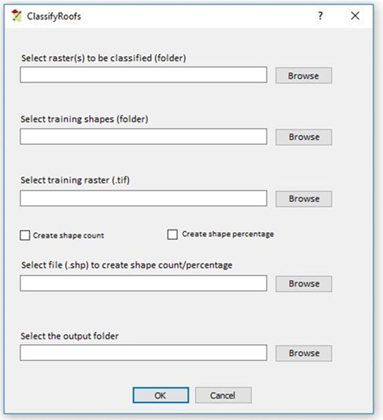
ISPRS Int. J. Geo-Inf. 2019, 8, 131                                                                   2 of 13

      There are different approaches that can be adopted for this reconnaissance. The use of remotely
sensed data has proven to be a good instrument for identifying and evaluating the status of roofing
made of asbestos fiber cement materials, e.g., by using images from space-borne remote sensing [4–8].
Due to the spectral characteristics of asbestos roofs, hyperspectral remotely sensed images are often
used for asbestos roofing identification [3,9–16].
      It is worthwhile to observe that space-borne sensors allow for a larger coverage area, and they can be
cheaper when compared with airborne sensors, such as the hyper-spectral sensor MIVIS (multispectral
infrared visible imaging spectrometer) [17]. Obviously, the use of imagery from space-borne sensors
means that the spatial and spectral resolution will be lower than with airborne sensors.
      Recent papers illustrate the possibility of exploiting remotely sensed images from sensors on
board the WorldView satellites. Pacifici shows that improvements in classification accuracy are
obtainable by using the WorldView-3 spectral bands, as compared with the more typical platforms [17].
Some researchers used an object-based approach to extract information from the images and have
proven that their processing methods have the potential to detect roof materials from the WorldView-2
images [18,19]. More recently, other authors have illustrated research carried out with discriminant
function analysis (DFA) and random forest (RF) on WorldView-2 imagery [20]. Their aim was to reveal
the efficiency of these classifiers, and the efficiency of pansharpening. The best results were gained by
RF, with both three and six classes. The results of the last paper confirm some choices that were made
during our research.
      This work arises from this context, and its goal is to provide a directory where all of the buildings
with asbestos cladding can be listed for a given area. To meet this requirement, this paper proposes a
low-cost tool that is designed to automatically identify buildings with asbestos roofing in a particular
area. Its task is to identify asbestos cladding in remotely sensed images, but not to classify the different
types of roofing. The tool is designed as a QGIS plugin, named ‘RoofClassify’. QGIS is an open source
geographic information system licensed under the GNU General Public License [21]. The version
used in this work is QGIS 2.18. The same tool presented here should make it possible in the future to
monitor the entire process of asbestos roofing removal in a selected area over time, and by means of
subsequent digital imaging.
      In the framework of this application, the considered area is the large metropolitan area around
Prato, which is the second most populated city in Tuscany (Italy). Images acquired by the WorldView-3
sensor were selected and processed. It is known that classifying these images is a difficult task, because
urban areas are characterized by different surface features that have similar spectral responses [22].
The probability of incorrectly classifying these surfaces thus increases. Traditional pixel-based
classifications seem unsuitable, whereas object-oriented classifications are more advisable [18,19,23].
      The RoofClassify plugin uses data integration techniques (vector and raster) for representing
WorldView-3 data onto a common grid. It then selects building-objects using vector format features,
and it finally applies a classification procedure to the roofing of buildings. The result of this process
is a new feature for each building-object. This feature is immediately usable within the integrated
geographic information system (GIS) environment for the analysis of each point characteristic (vector
and raster information), and for a statistical survey of the observed area.
      This approach makes it possible to filter the images without using, or training, object-oriented
classification algorithms or neural networks [20]. Moreover, it makes it possible to reduce errors due
to false positives that are represented by objects like asphalt on roads. Finally, fast software packages
can be used that are specifically designed for classifying pixel-based images.
      Section 2 focuses on the justification of the choice of images classified. The same section presents
the method used to detect Eternit cladding, and the designed open source software tool. The results
obtained, and the explanations of the validations, are reported in Section 3.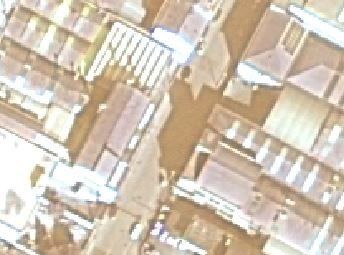
ISPRS Int. J. Geo-Inf. 2019, 8, 131                                                                   3 of 13

2. Materials and Methods

2.1. Roofing Classification
     The roofing classification was performed through digital image processing within the selected
area. The first step involved the kinds of images that the proposed software tool could be applied to.

2.1.1. Image Selection and Preprocessing
     The following systems were among the different aerial images that were used to reproduce the
Prato municipal district area:

•     Orthophoto: aerial photographs or images that have been geometrically corrected and
      georeferenced (“orthorectified”), with radiometric resolution in four spectral bands (R,G,B, NIR)
      and with a spectral coverage of up to ~800 nm. Such images are available free of charge at the
      Geoscope Observatory in Tuscany (http://www502.regione.toscana.it/geoscopio/ortofoto.html).
      Their low spectral resolution does not make it possible for their use in any asbestos classification.
•     Vector graphics files, available at the Geoscope Observatory in Tuscany. Once the Geoscope website
      is accessed, the layer with the information requested can be chosen; for instance, surveyor maps.
•     High spectral resolution images, acquired by airborne sensors (MIVIS) [14]. They are very
      expensive if there are specific acquisition procedures. Their broad representative potential is
      limited by the noise occurring in high-depth bands.
•     Satellite images acquired by the WorldView-3 sensor working on eight spectral bands. WorldView
      satellite imagery is often more expensive than RGB aerial imagery if a comparison is made between
      the archives. In the presented case, no archive aerial imagery is available, and additionally,
      WorldView images of the area of interest can be purchased at fairly low prices (about 2200 euros) [24].

      The need to have multispectral imaging and high spatial resolution [25] while trying to keep
costs down, influenced the choices of the images to be used for this research, favoring those that
were obtained by the WorldView-3 sensor. This sensor, owned by DigitalGlobe, is mounted on a
commercial Earth observation satellite [24]. In August 2014, DigitalGlobe launched this multi-payload,
super-spectral, very high spatial resolution satellite. Operating at an altitude of 620 km, WorldView-3
acquires panchromatic imagery at a 0.31 m maximum spatial resolution, eight visible and near-infrared
(VNIR) bands at 1.24 m maximum spatial resolution, and eight short-wave infrared (SWIR) bands at
3.7 m [17]. Since these images do not cover the asbestos emissions wavelength, it was possible to detect
the fiber-cement roofing by analyzing the corresponding spectrometric signature, namely, by analyzing
the typical reflection characteristics of this material to such wavelengths. Therefore, the classification
process was adjusted accordingly, so as to fully exploit each and every piece of information that could
be obtained from the available satellite images.
      Figure 1 shows the steps of the classification process, organized in a block diagram.
ISPRS Int. J. Geo-Inf. 2019, 8, 131 4 of 13
ISPRS Int. J. Geo-Inf. 2019, 8, x FOR PEER REVIEW 4 of 13
Figure 1. Illustration of the different processing steps of the classification process. VNIR is visible
Figure 1. Illustration of the different processing steps of the classification process. VNIR is visible and
and near-infrared.
near-infrared.
Two phases made up the process. The first non-automatic phase focused on preprocessing the
Two data,
available phases
andmade up the three
it included process. The first non-automatic phase focused on preprocessing the
steps.
available data, and it included three steps.
1. Pansharpening, the process that enabled a merger of the information collected from satellite
1. Pansharpening, the process that enabled a merger of the information collected from satellite
imaging, as acquired by the WorldView-3 sensor, in order to create a single image with the
imaging, as acquired by the WorldView-3 sensor, in order to create a single image with the
resolution of the initial panchromatic image (Figure 2). The low-resolution image was interpolated
resolution of the initial panchromatic image (Figure 2).
with bi-cubic interpolation. In this activity, pansharpening was carried out using a component
substitution algorithm. The, RCS (relative component substitution) algorithm was selected among
those available, through Orfeo Tool-box [26], a software integrated into QGIS. Table 1 describes
the features of the images used for such processing:
• A panchromatic image with a higher spatial resolution (50 cm);
• A multispectral image having eight spectral bands (coastal, blue, green, yellow, red, red
edge, NIR-1, NIR-2) and characterized by a spatial resolution of 2 m.
These images were georeferenced in UTM33 WGS84 and orthorectified. They were also calibrated
and corrected radiometrically. Our research started in 2016, and it aimed to document the
diffusion of asbestos roofs in the Prato area in 2014. For this reason, the selected images were
among those acquired in 2014. In fact, from that moment onwards, the authorities of Prato have
updated their database by inputting the removal procedures of asbestos-contaminated artifacts
by individuals and companies.
2. Raster image filtering, meaning filtering of the pixel grid, was obtained through a vector mask
of the chosen
Figurearea.
2. TheThe vector mask
multispectral imagewas something
obtained that ensued from
via pansharpening the cadastral
(resolution: 50 cm). shape layer,
namely, from the surveyor map where all of the buildings that were related to the selected
area were
The described viaimage
low-resolution a vector graphics
was editor (Figure
interpolated 3). Theinterpolation.
with bi-cubic inferred maskIn only
thiscontained
activity,
information that related
pansharpening was tocarried
the buildings’ roofing.
out using This processsubstitution
a component enabled the algorithm.
removal of everything
The, RCS
but(relative
the buildings’ roofing
component from the initial
substitution) satellitewas
algorithm image (Figureamong
selected 4). Thethose
cropping operation
available, was
through
performed using the
Orfeo Tool-box corresponding
[26], functions into
a software integrated offered by QGIS and based on the Gdal libraries.
QGIS.
Table 1 describes the features of the images used for such processing:ISPRS Int. J. Geo-Inf. 2019, 8, 131 5 of 13
3. Partition of the filtered image in tiles, namely sections that had suitable dimensions, so as to carry
out the classification as quickly as possible. The partition of the satellite image was carried out
with a plugin called GridSplitter, thus obtaining 49 sections, each of them correctly geo-referenced
according to the projection of the original image. Such tiles were saved into a single folder
containing only and exclusively these files.
Table 1. Characteristics of the satellite panchromatic image and of the multispectral image.
Description Panchromatic Image Multispectral Image
ortho14nov02101210-p2as-055 ortho14nov02101210-m2as-055
Image name
544307010_01_p001 544307010_01_p001
Source Planetek Italia Planetek Italia
Size 40785 × 25825 pixels 10197 × 6458 pixels
Imagine type Pancromatic Multispectral
Number of bands 1 8
Radiometric resolution (bit) 16 16
Figure 1. Illustration of the different processing steps of the classification process. VNIR is visible and
Spatial resolution (cm) 50 200
Acquisition date near-infrared.
02/11/2014 02/11/2014
Reference system Roma40/Ovest Roma40/Ovest
Two phases madetype
Resampling up the process. Bilinear
The firstInterpolation
non-automatic phase focused on preprocessing the
Bilinear Interpolation
Sensor
available data, and it included three steps. WorldView-3 WorldView-3
Cloud cover (%) 0 0
1. Pansharpening, the process that enabled a24.9
Off-nadir ◦
merger 24.9◦
of the information collected from satellite
Metadata
imaging, language by the WorldView-3
as acquired Italian
sensor, in order to create a singleItalian image with the
Character
resolution setinitial
of the code panchromatic imageutf-8 (Figure 2). utf-8
Figure 2. The multispectral image obtained via pansharpening (resolution: 50 cm).
The low-resolution image was interpolated with bi-cubic interpolation. In this activity,
pansharpening was carried out using a component substitution algorithm. The, RCS
(relative component substitution) algorithm was selected among those available, through
Orfeo Tool-box [26], a software integrated into QGIS.
Table 1 describes the features of the images used for such processing:namely, from the surveyor map where all of the buildings that were related to the selected area
were described via a vector graphics editor (Figure 3). The inferred mask only contained
information that related to the buildings’ roofing. This process enabled the removal of everything
but the buildings’ roofing from the initial satellite image (Figure 4). The cropping operation was
ISPRSperformed
Int. J. Geo-Inf.using
2019, 8,the
131corresponding functions offered by QGIS and based on the Gdal libraries.
6 of 13
Figure 3. Overlapping of the shapefile mask related to buildings, using the pansharpened satellite
ISPRSFigure 3. Overlapping
Int. J. Geo-Inf.
image excerpt.
of PEER
2019, 8, x FOR the shapefile
REVIEW mask related to buildings, using the pansharpened satellite6 of 13
image excerpt.
Mask filtering results related to the buildings involved.
Figure 4. Mask
2.1.2.Partition
3. Classification Procedure
of the filtered image in tiles, namely sections that had suitable dimensions, so as to carry out
the
Theclassification
second phase as quickly
was theasreal possible. The partition
classification of theofcladding
the satellite image was
available in thecarried
area out with a
according
to theplugin called GridSplitter,
pre-processed image. Digital thus image
obtaining 49 sections,
classification each of grouped
techniques them correctly geo-referenced
pixels into classes, to
according
represent to the projection
the different types of land of the
cover original image.were
data. There Suchthreetilesmain
wereapproaches
saved intoina digital
single image
folder
containingsupervised,
classification: only and exclusively
unsupervised,these files.
and object-oriented. The method applied hereafter was
based on supervised classification, which operated a per-pixel classification of the image with some
2.1.2. Classification
representative Procedure
samples, the true points, for each and every land cover data class that appeared in the
digital image. The
The second phase waschoice of athe
supervised approach was
real classification notcladding
of the limiting,available
because itinenabled
the areatheaccording
subsequent to
application
the of an object-oriented
pre-processed image. Digital classification, if required,
image classification as shown grouped
techniques further on. pixels into classes, to
In this
represent thecase study,types
different thereofwere
landsix selected
cover classes:
data. There asbestos
were three maincladding, fiber cement
approaches cladding,
in digital image
red/red roofing, black/shadow, green, and background. The last
classification: supervised, unsupervised, and object-oriented. The method applied hereafter class collected pixels from objects
was
that were
based different from
on supervised the roofing.which
classification, Theseoperated
pixels could be incorrectly
a per-pixel locatedofon
classification a building
the image with roofsome
due
to incorrect processing of the image, such as inaccurate georeferencing. The
representative samples, the true points, for each and every land cover data class that appeared in the white background pixels
of Figure
digital 4 also The
image. contributed
choice to of this class if the classification
a supervised approach was process also considered
not limiting, becausethem.it enabled the
subsequent application of an object-oriented classification, if required, as shown further on. a survey
The corresponding six training sets were composed of samples that were collected during
campaign
In thiscarried out in there
case study, the Prato
werearea. At each site,
six selected the geographical
classes: asbestos cladding, position
fiber(latitude,
cement longitude,
cladding,
WGS84
red/red datum)
roofing,of the surface was
black/shadow, detected,
green, and a link was
and background. Theassociated
last class with the vector
collected pixels record of the
from objects
building, as provided by the land registry.
that were different from the roofing. These pixels could be incorrectly located on a building roof due
The image
to incorrect classification
processing software
of the image, therefore
such worked
as inaccurate with the training
georeferencing. Thesets
white to define the kinds
background of
pixels
land
of cover4 in
Figure alsothecontributed
entire image. Digital
to this classimage
if theclassification
classificationdetermined
process alsothe membership
considered them.to each class
according to the “resemblance” of the observed object’s radiative properties
The corresponding six training sets were composed of samples that were collected during to the properties defined a
in the training set. Among the different algorithms operating supervised
survey campaign carried out in the Prato area. At each site, the geographical position (latitude, classifications, the random
forest algorithm
longitude, WGS84 was selected
datum) andsurface
of the appliedwas to the available
detected, andimages.
a link was Indeed, this algorithm
associated with theseemed
vector
record of the building, as provided by the land registry.
The image classification software therefore worked with the training sets to define the kinds of
land cover in the entire image. Digital image classification determined the membership to each class
according to the “resemblance” of the observed object’s radiative properties to the properties
defined in the training set. Among the different algorithms operating supervised classifications, theISPRS Int. J. Geo-Inf. 2019, 8, 131 7 of 13
to be more suitable, because as an ensemble of classifiers, it was capable of classifying each pixel by
resorting to its characteristics, such as: its spectral properties in the eight different bands of the satellite
sensor, its panchromatic value, and its membership to building class. Moreover, it worked well when
homogeneous training data were available, and it was relatively robust to outliers. Last, but not least,
implementation of this algorithm ensured a high computational speed [19,27–29]. Within this work,
the classification process was totally automatic, and it was implemented with an algorithm that was
specifically designed through a QGIS plugin.
2.2. The RoofClassify Plugin
The QGIS open source environment enables any data collection coming from different sources
(raster, vector, database, and so forth), to be used to build a single project of spatial analysis that
is capable of meeting the basic functionalities that a GIS has to cope with. Furthermore, a useful
aspect of QGIS is the option of expanding basic functionalities through plugins in Python language,
which is simple for any user to understand. This means that Python libraries that are related to both
image management and processing can interact with the functionalities that a GIS has (for instance
displaying an indexed map in some reference systems). This leads to the possibility of creating a
simple application that efficiently copes with a particular problem: the application software has a user
interface, and it works with both new and already existing application fields in QGIS, as defined by
the user in Python language.
The RoofClassify plugin was developed within the application field of this current paper, and
it made it possible to classify a pre-processed satellite image, as already described in Section 2.1.1.
The plugin outputs included both the image that had its pixels classified, and an optional shapefile
“describing” the outcome, which is to say, a shapefile having all of the pieces of information concerning
the number of pixels for each polygon in each class of the image. The percentage of pixels classified as
asbestos within each polygon was optionally reported.
2.2.1. Plugin User Interface (UI)
The assumption is based on having the initial image to be classified as something that is organized
in a single folder, which includes only the tiles that the image is made of, or the entire image itself.
Being a supervised classification, it is also assumed that the user has a raster with some true
points, namely, some buildings’ cladding in a definitely known material, which can be used as a
classification training set. Each single class is identified by a shapefile, with one different shapefile for
each class, thus uniquely identifying a type of cladding that is known in advance. These shapefiles are
saved, for convenience, in a single folder containing only such files.
In short, there must be:
• The image to be classified, whether it is single or divided into tiles, kept together in a single folder;
• A folder containing the shapes corresponding to each identified class;
• The image to be used as a training set, where different shapes are represented.
The plugin interface is depicted in Figure 5. The different items have the following meanings:
• Select raster(s) to be classified (folder): by selecting the ‘browse’ button, it is possible to search the
folder that has the image (or images) to be classified.
• Select training shapes (folder): by selecting the ‘browse’ button, it is possible to search the folder
that has shapefiles corresponding to the different classes of the training set.
• Select training raster (.tif): by selecting the ‘browse’ button, it is possible to search the geo-referenced
image (filename extension ‘.tif’) whose pixels conform to the shapefiles set out in point 2.
• Create shape count: by ticking this (which is optional), the plugin creates not only a classified image,
but also a shapefile (*.dbf) containing all of the polygons that correspond to each cladding. In this
shape, each polygon (building) is provided with the following information: the identificationISPRS Int. J. Geo-Inf. 2019, 8, 131 8 of 13
code, the total number of pixels that each polygon has, and the pixel number of each identified
class in the polygon.
• Create shape percentage: by ticking this (which is optional), the plugin creates not only a classified
image, but also a shapefile (*.dbf) containing all of the polygons that correspond to each
cladding. In this shape, each polygon (building) is provided with the following information: the
identification code, and the percentage of classified pixels within each polygon for each identified
ISPRSclass
Int. J. in
Geo-Inf.
that 2019, 8, x FOR PEER REVIEW
polygon. 8 of 13
• Select the file (.shp) to create a shape count/percentage: whether one of the two previously mentioned
• Select the file (.shp) to create a shape count/percentage: whether one of the two previously mentioned
options or both of them have been ticked, this box makes it possible to select the shapefile to be
options or both of them have been ticked, this box makes it possible to select the shapefile to be
used when calculating the required statistics. Generally speaking, this shapefile is the same as the
used when calculating the required statistics. Generally speaking, this shapefile is the same as
one that is used in the filtering phase of the satellite image.
the one that is used in the filtering phase of the satellite image.
• Select the output folder: when clicking on ‘browse’, it is possible to select the folder where the
• Select the output folder: when clicking on ’browse’, it is possible to select the folder where the
output files will be saved.
output files will be saved.
Figure 5. User Interface of the RoofClassify
Figure 5. RoofClassify plugin.
plugin.
2.2.2. Focusing on How the Classification Plugin is Organized
2.2.1. Focusing on How the Classification Plugin is Organized
The plugin performs the classification according to the following procedural points:
The plugin performs the classification according to the following procedural points:
1.
1. Importing the
Importing theraster
rasterimage
image to to
be be
classified (images
classified available
(images in thein
available selected folder as
the selected inputas
folder dataset)
input
into a Python data structure (multi-array), where each and every pixel matches exactly
dataset) into a Python data structure (multi-array), where each and every pixel matches exactly with a cell
of thea structure,
with cell of themade of eight
structure, madecomponents (one for each
of eight components band).
(one for each band).
2.
2. Importing the raster image, which represents the selected training
Importing the raster image, which represents the selected training set
set for
for classification
classification purposes
purposes
(same as point
(same as point 1). 1).
3.
3. Extracting the
Extracting thetraining
trainingsetset
from the the
from shapefile: a shapefile
shapefile: is defined
a shapefile for eachfor
is defined class to beclass
each identified,
to be
and it includes
identified, and the polygonsthe
it includes matched
polygonswithmatched
the related roofing.
with As previously
the related roofing.explained, each
As previously
explained, each and every shape (one shape matching with the asbestos class, one shape for a
red roof, and so forth) is saved in a single folder. The algorithm will recursively access this
folder, looking for the shapes in order to extract the training set. These data are also imported
into a Python multiarray.
4. Training the classifier file: the training and classification algorithm belongs to the “Scikit-learn”ISPRS Int. J. Geo-Inf. 2019, 8, 131 9 of 13
and every shape (one shape matching with the asbestos class, one shape for a red roof, and so
forth) is saved in a single folder. The algorithm will recursively access this folder, looking for the
shapes in order to extract the training set. These data are also imported into a Python multiarray.
4. Training the classifier file: the training and classification algorithm belongs to the “Scikit-learn”
Python library. The multiclass “RandomForest” classification function was used in this case,
which was more suitable for execution speed. The inputs were: the multiarray raster of the
ISPRS Int. J. Geo-Inf. 2019, 8, x FOR PEER REVIEW 9 of 13
training set (point 2); the multiarray shapes of the training set (point 3).
5.
5. Classification
Classification according
according to to the
the selected
selected function.
function. The
The output
output will
will be
be aa multiarray
multiarray comprising
comprisingthe
the
classified pixels’ values.
classified pixels’ values.
6.
6. Reconstructing and saving the correctly geo-referenced image as the starting image for use,
beginning with the output provided in point point 5.
5.
Some items
Some items were
were left
left out
out of
of the
the above
above description
description for
for the
the sake
sake of
of brevity,
brevity, namely,
namely, the
the option
option of
of
creating the shapefile with all of the information on classification.
creating the shapefile with all of the information on classification.
3. Classification
3. ClassificationResults
Resultsand
andValidation
Validation
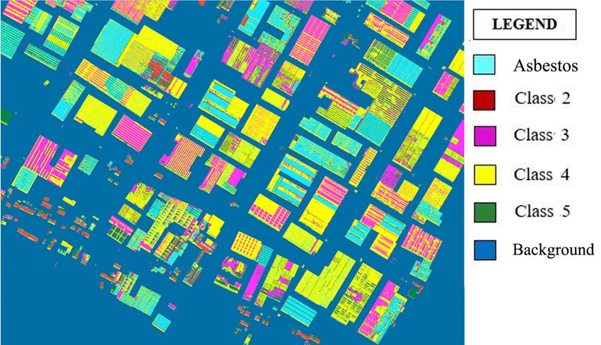
The outcome
The outcome that
that is
is achieved
achieved by by applying
applying the the plugin
plugin to
to the
the pre-processed
pre-processed image
image is
is an
an image
image
that has
that has pixels
pixels classified
classified according
according to to the
the different
different types
types of
ofroofing.
roofing. Such
Such an
an image
image isis correctly
correctly
geo-referenced according
geo-referenced according to to the
the source
source satellite
satellite image.
image. Figure 6 is is an
an example
example of
of aa part
part of
of an
an image
image
with classified pixels.
with classified pixels.
Figure 6. A
Figure 6. A part
part of
of aa classified
classified image.
image.
With
Withregard
regardto toeach
eachbuilding
buildingininthe
theinput
inputshape
shape file
file(Shapefile
(ShapefileMask),
Mask), once
once thethe classified
classified image
image
is
is available, the designed algorithm identifies the total number of pixels in that image, and
available, the designed algorithm identifies the total number of pixels in that image, and for
for each
each
identified class, the total number of pixels belonging to that specific
identified class, the total number of pixels belonging to that specific class. class.
When
When thethe classification
classification is
is complete,
complete, the
the worthiness
worthiness ofof such
such aa process
process needs
needs to to be
be demonstrated,
demonstrated,
by
by validating its outcome. However, given the nature of this use, specifically, the lack
validating its outcome. However, given the nature of this use, specifically, the lack of
of sufficient
sufficient
samples of a well-known nature, especially in dealing with asbestos as the class
samples of a well-known nature, especially in dealing with asbestos as the class of interest, of interest, it becomesit
more and more difficult to carry out validations with the criteria and techniques that
becomes more and more difficult to carry out validations with the criteria and techniques that are are most common
in the common
most literature.in the literature.
Therefore, the following actions were performed to verify the worthiness of this classification
method:
1. Identifying the building roofing with well-known construction materials as well as their
tagging according to the corresponding class.
2. Creating a shapefile for each class, which included the previously tagged roofing types for eachISPRS Int. J. Geo-Inf. 2019, 8, 131 10 of 13
Therefore, the following actions were performed to verify the worthiness of this classification method:
1. Identifying the building roofing with well-known construction materials as well as their tagging
according to the corresponding class.
2. Creating a shapefile for each class, which included the previously tagged roofing types for each
file, according to a specific class.
3. Developing a Python script. Provided with input data, which consisted of both the image created
from the classification process, and the shapefiles, as described in point 2, this script is capable of
providing a confusion matrix as an output.
4. Analyzing the confusion matrix and estimating any possible classification errors.
The first phase is very critical, and it draws the line at the validation process; in fact, the
classification process classifies each pixel according to the dominantly present classes, but an ambiguity
arises when asbestos and fiber cement classes are concerned. Indeed, there is a problem with correctly
allocating the tag “cement” or “asbestos” to pixels belonging to the available images.
The action taken in order to address a similar situation for such surfaces was to use the
corresponding “true points”—obviously not the ones selected for the training set—as test buildings
for the asbestos class. Other asbestos-free, newly registered, and recently built structures were used as
test buildings for the cement class.
The outcomes are described in Table 2, which represents the confusion matrix, or the taking into
account of the outcomes of mistaken classification relating to the parts of the image: the first-line
cells show the true classes, whereas the first-column cells show the output classes according to the
classification tool. There were six true/output classes of this matrix, according to the number of classes
that collected roofing and background.
Table 2. Confusion matrix. CA is commission accuracy, OA is omission accuracy.
Asbestos Cement Black/Shadow Green Background Red OA (%)
Asbestos 13,992 4036 120 39 17 422 75.12
Cement 682 9779 321 252 0 126 87.63
Black/Shadow 1 88 706 9 0 1 87.70
Green 368 544 140 2312 1 173 65.35
Background 0 0 0 0 1346 0 100
Red 415 853 486 150 120 13,867 87.26
CA (%) 90.52 63.91 39.82 83.71 90.70 95.5 81.77
In this regard, if an “i” index is assigned to the seven rows representing true classes, and a “j”
index is also assigned to the seven output classes, the cell corresponding to the “i”-indexed row and
the “j”-indexed column shows the number of pixels that are labeled as belonging to the “j”-indexed
class, according to the classification process, whereas in reality they belong to the “i”-indexed class.
In order to evaluate the quality of the results, the eighth row and the eighth column were added,
respectively containing the percentage values of the commission accuracy (CA), namely, the user’s
accuracy, and the omission accuracy (OA) [30]. Errors of omission represented false negatives. Errors
of commission represented false positives. The overall or average accuracy was 81.77% (reported at
the bottom right corner of the matrix). The Kappa index of the classifier was 0.7514 [31].
As evident from the table, many pixels belonging to “cement” and “asbestos” classes were used
in this test, with respect to other classes like “green” or “shadow”. This choice was motivated by the
classification method, which focused on asbestos detection. Therefore, when calculating the process
accuracy, greater consideration should have been given to the class to be detected, as well as to the
other classes that asbestos could have been misclassified with.
It turns out that the percentage of correction classification that was related to asbestos detection
amounted to 75.12% when analyzing the confusion matrix.ISPRS Int. J. Geo-Inf. 2019, 8, 131 11 of 13
Another validation was carried out on the basis of the data collected in the Health Information
System for Collective Prevention (SISPC) [32], which is a regional database that provides the
stake-holders with a tool to manage health activities and data in a uniform way throughout the
regional territory. Clean-up plans, as well as removal and disposal procedures of products and artifacts
contaminated with asbestos, are presented online, by means of the SISPC. Therefore, this system
provided data with the highest “evidentiary” value, which was needed for a complete validation of
the classification data. A validation of the SISPC data was carried out by visual examination, where
the related depollution location was checked via Google maps, by identifying the roofing that could
be consistent with the declared remediation, and by verifying whether the classification, previously
carried out on the image before any clean-up operation, had detected asbestos in that area. A selection
was made for both residential and industrial buildings, with 11 different addresses. As for classification
accuracy, the results on asbestos-classified pixels were better than the outcome obtained with the
previously explained validation method. Indeed, the plugin RoofClassify detected 90% of asbestos
roofs. The differences between the validation tests lied in the lower spectral ambiguities of the selected
buildings in the second validation procedure.
4. Discussion
The QGIS tool described in this paper was conceived for identifying building roofs with asbestos.
Roofing classification was performed through the digital processing of images obtained by the
WorldView-3 sensor. Such images were pre-processed, so as to make them suitable for subsequent
classification [20]. The outcomes, as achieved in an open context, underwent a validation process,
which consisted of analyzing the confusion matrix, and subsequently assessing the classification
errors. Given that the most difficult task was testing the tool’s impact in discerning asbestos and
cement, the decision was made to only use structures with well-known roofing materials as the test
buildings, according to recent surveys [18–20]. A second validation was carried out on the basis
of a verification process, with data being collected at the Health Information System for Collective
Prevention (SISPC) [32].
The results obtained from the first validation showed that about 25% of the asbestos roofing was
a false negative. At the same time, a high number of asbestos pixels were classified as cement pixels,
because asbestos-reinforced cement often contains only 6% of asbestos fiber. These observations could
lead to the conclusion that a weak performance by the classification method was obtained [20,30].
Improvements in asbestos roofing identification are possible when resorting to object-oriented
classification [22]. As previously mentioned, the designed algorithm identifies the total numbers of
pixels in that image, and the total number of pixels belonging to each specific class. The plugin can also
compose an optional shapefile that describes all of the pieces of information concerning the number of
pixels in each class, for each polygon that composes the images. Optionally, the plugin provides the
percentage of pixels that are classified as asbestos, within each polygon. This optional shapefile makes
it possible to estimate the probability that a building has asbestos roofing. Therefore, it is possible
to assign the “asbestos” or “not asbestos” labels to each roof. This procedure should significantly
improve classification performance. This last step is left to the user, who can visualize the data that is
extracted from the algorithm.
The tool for asbestos identification in the QGIS platform requires a basic grasp of GIS, but the
open-source environment makes it easier for both software use and algorithm distribution. A plugin
limit is built into the algorithm, which is conceived to only identify asbestos. Strictly speaking, this
feature cannot be considered a flaw, nor a limit on flexibility: in fact, the plugin is meant to perform
a specific classification of asbestos, and it has been optimized for this individual purpose, making it
different from other proprietary software.ISPRS Int. J. Geo-Inf. 2019, 8, 131 12 of 13
5. Conclusions
This paper has focused on an asbestos identification system to give support to the asbestos roofing
disposal policies and programs in small geographical areas. The classification tool is based on GIS
open source software, and it was used to analyze Prato district satellite images obtained with the
WorldView-3 sensor. The QGIS tool has shown quite good performance in identifying asbestos roofing
when applying a per-pixel classification. The percentage of asbestos pixels contained in each roof of
the analyzed image can also be determined with this tool. This value can be used for improving the
classification process. The presented classification methods can be explained in terms of restoring a
data sheet, or a list of records on asbestos roofing buildings, and it can provide a low-cost basis for
building up a larger knowledge database, where geographical data are integrated with other data from
different administrative sources (as, for instance, SISPC).
Author Contributions: Conceptualization, Maurizio Tommasini and Monica Gherardelli; methodology,
Maurizio Tommasini; software, Alessandro Bacciottini; validation, Alessandro Bacciottini; formal analysis,
Maurizio Tommasini and Monica Gherardelli; data curation, Alessandro Bacciottini; writing—original draft
preparation and editing, Monica Gherardelli; supervision, Maurizio Tommasini and Monica Gherardelli.
Funding: This research was funded by the MUNICIPALITY OF PRATO. The APC received no external funding.
Conflicts of Interest: The authors declare no conflict of interest. The funder had no role in the design of the study;
in the collection, analyses, or interpretation of data; or in the writing of the manuscript. The funder approved the
publication of the results.
References
1. Bartrip, P.W.J. History of asbestos related disease. Postgrad. Med. J. 2004, 80, 72–76. Available online:
https://pmj.bmj.com/content/postgradmedj/80/940/72.full.pdf (accessed on 1 February 2019).
2. Suzuki, Y.; Yuen, S.R.; Ashley, R. Short, thin asbestos fibers contribute to the development of human
malignant mesothelioma: pathological evidence. Int. J. Hyg. Environ. Healt 2005, 208, 201–210. [CrossRef]
[PubMed]
3. Szabó, S.; Burai, P.; Kovács, Z.; Szabó, G.; Kerényi, A.; Fazekas, I.; Paládi, M.; Buday, T.; Szabó, G. Testing
Algorithms for the Identification of Asbestos Roofing Based on Hyperspectral Data. Environ. Eng. Manag. J.
2014, 143, 2875–2880. [CrossRef]
4. Barrile, V.; Bilotta, G.; Pannuti, F. A Comparison Between Methods—A Specialized Operator, Object
Oriented and Pixel-Oriented Image Analysis—To Detect Asbestos Coverages in Building Roofs Using
Remotely Sensed Data. In Proceedings of the International Archives of the Photogrammetry, Remote Sensing
and Spatial Information Sciences, XXI ISPRS Congress, Beijing, China, 3–11 July 2008; Volume XXXVII,
pp. 427–434. Available online: http://www.isprs.org/proceedings/XXXVII/congress/8_pdf/2_WG-VIII-2/
51.pdf (accessed on 22 January 2019).
5. Bhaskaran, S.; Paramananda, S.; Ramnarayan, M. Per-Pixel and Object-Oriented Classification Methods for
Mapping Urban Features Using Ikonos Satellite Data. Appl. Geogr. 2010, 30, 650–665. [CrossRef]
6. Taherzadeh, E.; Shafri, H.Z.M.; Mansor, S.; Ashurov, R. A comparison of hyperspectral data and WorldView-2
images to detect impervious surface. In Proceedings of the 2012 4th Workshop on Hyperspectral Image and
Signal Processing (WHISPERS), Shanghai, China, 4–7 June 2012; pp. 1–4. [CrossRef]
7. Ban, Y.; Jacob, A.; Gamba, P. Spaceborne SAR Data for Global Urban Mapping at 30m Resolution Using a
Robust Urban Extractor. ISPRS J. Photogramm. Remote Sens. 2015, 103, 28–37. [CrossRef]
8. Samsudin, S.H.; Shafri, H.Z.M.; Hamedianfar, A. Development of Spectral Indices for Roofing Material
Condition Status Detection Using Field Spectroscopy and Worldview-3 Data. J. Appl. Remote Sens. 2016, 10,
025021–025038. [CrossRef]
9. Marino, C.M.; Panigada, C.; Busetto, L. Airborne hyperspectral remote sensing applications in urban areas:
Asbestos concrete sheeting identification and mapping. In Proceedings of the IEEE/ISPRS Joint Workshop
on Remote Sensing and Data Fusion over Urban Area, Rome, Italy, 8–9 November 2001; pp. 7541–7544.
10. Fiumi, L. Evaluation of MIVIS Hyperspectral Data for Mapping Covering Materials. In Proceedings of
the IEEE/ISPRS Joint Workshop on Remote Sensing and Data Fusion over Urban Areas, Rome, Italy, 8–9
November 2001; pp. 324–327.ISPRS Int. J. Geo-Inf. 2019, 8, 131 13 of 13
11. Bassani, C.; Cavalli, R.M.; Cavalcante, F.; Cuomo, V.; Palombo, A.; Pascucci, S.; Pignatti, S. Deterioration
Status of Asbestos-Cement Roofing Sheets Assessed by Analyzing Hyperspectral Data. Remote Sens. Environ.
2007, 109, 361–378. [CrossRef]
12. Fiumi, L.; Campopiano, A.; Casciardi, S.; Ramires, D. Method Validation for the Identification of
Asbestos–Cement Roofing. Appl. Geomat. 2012, 4, 55–64. [CrossRef]
13. Frassy, F.; Candiani, G.; Maianti, P.; Marchesi, A.; Nodari, F.R.; Rusmini, M.; Albonico, C.; Gianinetto, M.
Airborne Remote Sensing for Mapping Asbestos Roofs in Aosta Valley. In Proceedings of the IEEE
International Geoscience and Remote Sensing Symposium (IGARSS 2012), Munich, Germany, 22–27 July
2012; pp. 7541–7544.
14. Frassy, F.; Candiani, G.; Rusmini, M.; Maianti, P.; Marchesi, A.; Rota Nodari, F.; Dalla Via, G.; Albonico, C.;
Gianinetto, M. Mapping Asbestos-Cement Roofing with Hyperspectral Remote Sensing over a Large
Mountain Region of the Italian Western Alps. Sensors 2014, 14, 15900–15913. [CrossRef] [PubMed]
15. Fiumi, L.; Congedo, L.; Meoni, C. Developing Expeditious Methodology for Mapping Asbestos-Cement
Roof Coverings over the Territory of Lazio Region. Appl. Geomat. 2014, 6, 37–48. [CrossRef]
16. Cilia, C.; Panigada, C.; Rossini, M.; Candiani, G.; Pepe, M.; Colombo, R. Mapping of Asbestos Cement Roofs and
Their Weathering Status Using Hyperspectral Aerial Images. ISPRS Int. J. Geo-Inf. 2015, 4, 928–941. [CrossRef]
17. Pacifici, F. On the Predictive Value of the WorldView3. VNIR and SWIR Spectral Bands. In Proceedings of
the IEEE International Geoscience and Remote Sensing Symposium (IGARSS 2016), Beijing, China, 10–15
July 2016; pp. 898–901. [CrossRef]
18. Taherzadeh, E.; Shafri, H.Z.M. Development of a Generic Model for the Detection of Roof Materials Based
on an Object-Based Approach Using Worldview-2 Satellite Imagery. Adv. Remote Sens. 2013, 2, 312–321.
[CrossRef]
19. Gibril, M.B.A.; Shafri, H.Z.M.; Hamedianfar, A. New semi-automated mapping of asbestos cement roofs
using rule-based object-based image analysis and Taguchi optimization technique from WorldView-2 images.
Int. J. Remote Sens. 2017, 38, 467–491. [CrossRef]
20. Abriha, D.; Kovács, Z.; Ninsawat, S.; Bertalan, L.; Balázs, B.; Szabó, S. Identification of roofing materials with
Discriminant Function Analysis and Random Forest classifiers on pan-sharpened WorldView-2 imagery—A
comparison. Hung. Geogr. Bull. 2018, 67, 375–392. [CrossRef]
21. QGIS. Available online: https://qgis.org/en/site/forusers/download.html (accessed on 15 January 2019).
22. Myint, S.W.; Gober, P.; Brazel, A.; Grossman-Clarke, S.; Weng, Q. Per-Pixel vs. Object-Based Classification
of Urban Land Cover Extraction Using High Spatial Resolution Imagery. Remote Sens. Environ. 2011, 115,
1145–1161. [CrossRef]
23. Blaschke, T. Object based image analysis for remote sensing. ISPRS J. Photogramm. Remote Sens. 2010, 65,
2–16. [CrossRef]
24. Digital Globe. Available online: https://www.digitalglobe.com/ (accessed on 22 January 2019).
25. Jenson, J.R.; Cowen, D.C. Remote sensing of urban/suburban infrastructure and socio-economic attributes.
Photogramm. Eng. Remote Sens. 1999, 65, 611–622.
26. Orfeo Tool-Box. Available online: https://www.orfeo-toolbox.org/ (accessed on 22 January 2019).
27. Kulkarn, A.D.; Lowe, B. Random Forest Algorithm for Land Cover Classification. Int. J. Recent Innov. Trends
Comput. Commun. 2016, 4, 58–63.
28. Whitcomb, J.; Moghaddam, M.; McDonald, K.; Kellndorfer, J.; Podest, E. Wetlands Map of Alaska Using
L-Band Radar Satellite Imagery. Can. J. Remote Sens. 2009, 35, 54–72. [CrossRef]
29. Tso, B.; Mather, P. Classification Methods for Remotely Sensed Data; Taylor & Francis: London, UK, 2001;
pp. 309–326.
30. Richards, J.A. Classifier performance and map accuracy. Remote Sens. Environ. 1996, 57, 161–166. [CrossRef]
31. Mclver, D.K.; Friedl, M.A. Estimating pixel-scale land cover classification confidence using nonparametric
machine learning methods. IEEE Trans. Geosci. Remote Sens. 2001, 39, 1959–1968. [CrossRef]
32. SISPC—Tuscany Region. Available online: http://opendata.prevenzionecollettiva.toscana.it/ (accessed on
15 January 2019).
© 2019 by the authors. Licensee MDPI, Basel, Switzerland. This article is an open access
article distributed under the terms and conditions of the Creative Commons Attribution
(CC BY) license (http://creativecommons.org/licenses/by/4.0/).You can also read