Vibration energy harvesters with optimized geometry, design, and nonlinearity for robust direct current power delivery
←
→
Page content transcription
If your browser does not render page correctly, please read the page content below
Smart Materials and Structures

PAPER

Vibration energy harvesters with optimized geometry, design, and
nonlinearity for robust direct current power delivery
To cite this article: Wen Cai and Ryan L Harne 2019 Smart Mater. Struct. 28 075040

View the article online for updates and enhancements.

                            This content was downloaded from IP address 140.254.87.149 on 24/06/2019 at 22:28
Smart Materials and Structures
Smart Mater. Struct. 28 (2019) 075040 (16pp) https://doi.org/10.1088/1361-665X/ab2549
Vibration energy harvesters with optimized
geometry, design, and nonlinearity for
robust direct current power delivery
Wen Cai and Ryan L Harne
Department of Mechanical and Aerospace Engineering, The Ohio State University, Columbus, OH 43210,
United States of America
E-mail: harne.3@osu.edu
Received 14 March 2019, revised 27 April 2019
Accepted for publication 29 May 2019
Published 18 June 2019
Abstract
With an ever-growing Internet-of-things, vibration energy harvesting has attracted broad
attention to replace consumable batteries to power the many microelectronic devices. To this
end, an energy harvester must deliver the required power to an electrical load over a long time
horizon. Yet, design practices for energy harvesters often report strategies based on maximizing
output voltage and wide frequency range of operation, which is not directly related to
performance-robust functioning. Motivated to provide valuable insight to practical development
of vibration energy harvesters, this research develops an analytical modeling framework and
optimization technique to guide attention to piezoelectric laminated energy harvesting
cantilevers with balanced and robust performance characteristics. The model is numerically and
experimentally validated to confirm the efficacy of the optimization outcomes. The results
indicate that laminated trapezoidal beam shapes with monostable configuration are the best
solution to broaden the frequency range of enhanced dynamic behavior, minimize strain at the
clamped beam end, and maximize the output voltage in a rectifier circuit. The results also find
that the selection of tip mass may not be highly influential for the overall performance so long as
the beam shape, beam length, and placement of nonlinearity-induced magnets are appropriately
chosen.
Keywords: laminated piezoelectric beam, multi-objective optimization, vibration energy
harvesting, genetic algorithm
(Some figures may appear in colour only in the online journal)
1. Introduction over a long time horizon, is therefore central to the vision of a
sustainable IoT [4].
With an accelerating development of the Internet-of-things The fundamental requirement of a vibration energy har-
(IoT), sustainably powering the vast fleet of low-power vester is to ensure the necessary DC power is delivered to an
wireless devices in our world is on the verge of crisis [1]. electrical load. Optimization strategies therefore seek to
With a projected growth of IoT devices upwards of tens of enable this requirement. A straightforward method to max-
billions by 2020 [2], the excessive reliance on chemical bat- imize output power is to increase the electromechanical
teries threatens the environment and resilience of the global coupling coefficient for a piezoelectric harvester platform,
energy economy. Yet, vibrational energy harvesting suggests which enhances the conversion efficiency between vibration
a promising solution to meet a portion of the accelerating and electrical energies. Cho et al [5] uncovered the influences
power supply demand [3]. Optimizing such vibration energy of residual stress, layering thicknesses, and electrode cover-
harvester platforms to ensure robust direct current (DC) age on the resulting electromechanical coupling coefficient
power when subjected to broadband vibration excitation, and for an optimized thin-film PZT membrane design. Wang and
0964-1726/19/075040+16$33.00 1 © 2019 IOP Publishing Ltd Printed in the UKSmart Mater. Struct. 28 (2019) 075040 W Cai and R L Harne
Wu [6] examined the effects of the piezoelectric patch posi-
tioning and size for application on a cantilever beam, to show
how power harvesting efficiency could be optimized. Lü et al
[7] proposed an optimization method by introducing an
intrinsic power density scale to reduce the number of para-
meters for optimizing energy conversion efficiency. Qin et al
[8] investigated the influence of dimensions on the PZT-5A
material and arrived at an optimal electromechanical coupling
coefficient (k15) for the shear vibration mode of energy har-
vesting. In addition, after identifying the superiority of a
trapezoidal piezoelectric beam shape for mechanical robust-
ness and long service life [9], alternative tapered beam shapes
have been studied to enhance the uniformity of strain dis-
tribution along the beam length [10–14]. Dietl and Garcia
[15] developed an optimization tool on the basis of such Figure 1. (a) Schematic of nonlinear energy harvester system with
repulsive magnets and rectification circuit interface. (b) Dimensions
trends and proposed an optimal curved piezoelectric beam
of the piezoelectric beam. (c) Cross-section of the piezoelectric beam
shape for more uniform strain distribution. Further approa- among the several layers.
ches to the beam configuration have been considered for the
sake of maximizing electrical power generation, for example in high bending strain. Without cautious design, a piezo-
a tapered beam with cavity [16], right-angle piezoelectric electric energy harvester could fail in hours, or even in
cantilevers having auxiliary beams [17], beams with initial minutes [33–35]. Gundimeda et al [36] have helped quantify
curvature [18], and piezoelectric energy harvesters having the mechanical robustness and design flexibility of laminated
cellular honeycomb structures [19]. beams when compared with conventional metal substrates
Because linear dynamic response only ensures high used for piezoelectric beams. Li et al [37] further demon-
output power around the primary resonant frequencies, robust strated the superiority of laminated piezoelectric beams to
electrical power delivery must involve an energy harvester yield high output power. Yet, strain conditions or laminated
exhibiting large amplitude dynamic behaviors when subjected beams are seldom considered when optimizing the energy
to broadband frequency vibration excitation. One well-known harvester, especially if nonlinearity is introduced.
method to broaden the frequency range of a piezoelectric Given the state-of-the-art in optimization efforts for
energy harvester is to introduce nonlinear magnetic effects piezoelectric energy harvesters, a need exists to develop an
[20–22]. Erturk and Inman [23] suggested as much as an optimization approach that exploits nonlinearity in the design
800% increase in output power could be achieved for a bis- of custom-shaped harvesters having excellent DC output
table magnetopiezoelastic harvester under harmonic vibration power, broad frequency range of operation, and exceptional
when the platform was interfaced with a purely resistive mechanical robustness. This research meets the need via an
electrical load. Comparatively, Ferrari et al [24] reported a analytical model and integrated genetic algorithm (GA)
250% increase in output power for a magnetoelastic energy optimization framework. The following sections introduce the
harvester subjected to wideband stochastic excitation. The analytical method, numerically verify the efficacy of the
frequency range for large amplitude response and large output analysis, and then establish the optimization framework.
power has been extended also by adopting adaptive bistable Optimized piezoelectric energy harvesters are then examined
harvester designs to more often realize the snap-through and cross-compared, after which an experimental sequence
behavior [25–27]. In this spirit, Zhou et al [28] proposed a confirms the validity of the theoretical predictions through
flexible bistable energy harvester with two elastic beams to laboratory examinations. A summary of main discoveries
create a variable repulsive magnetic force, which may reduce from this research are presented to conclude this report.
the potential barrier that must be overcome to ensure snap-
through oscillation. Recently instead of focusing on the bis-
table system, multi-stable systems, such as tri-stable energy
harvester, have been introduced to enhance the frequency 2. Analytical model overview
range and output power achieved for the large amplitude
dynamic behaviors [29, 30]. Because the alternating current
2.1. Analytical model formulation for a laminated piezoelectric
output from the harvester must be rectified to DC to power
beam with magnetic nonlinearity
electronic devices, nonlinear harvester platforms interfaced
with rectifier circuits [31] or power management circuits [32] Figure 1 presents a schematic of the nonlinear energy har-
have also demonstrated broadband frequency response vesting system considered in this research. A laminated
despite interfacing with such nonlinear electrical circuits. piezoelectric cantilever is interfaced with a rectifier bridge Di,
Yet, enhanced dynamic behavior may correspondingly smoothing capacitor CL, and load resistance R, which is a
be detrimental to the long working life of the vibration energy standard energy extraction circuit. The lamination sequence is
harvester. In particular, the PZT material is exceedingly brittle intricate. As shown in figure 1(b), along the total length L of
such that it is vulnerable to damage caused by events resulting the clamped beam, the width at the free end bL and the width
2Smart Mater. Struct. 28 (2019) 075040 W Cai and R L Harne
at the fixed end b0 are the layers D, composed from a glass- velocity at the mass center. The distance from the laminated
reinforced epoxy laminate (FR4). The thickness of the FR4 is beam end to the mass center of the holder is dc as shown in
2hs. Since ceramic materials are exceedingly difficult to figure 1(a)
arbitrarily shape due to extreme brittleness, here we consider
1
a piezoelectric PZT-5H layer labeled as layer B that adopts a Tm = M0 [w (L + dc, t ) + vb ]2
fixed and commercially available rectangular shape. The 2
subsequent optimization of this report considers other beam 1
= M0 [w (L, t ) + dc · w x (L, t ) + vb ]2 . (4 )
design parameters as candidates for optimization, in contrast 2
to change of the PZT-5H layer shape. The length, width, and
The w is the first derivative of the displacement with respect
thickness of the piezoelectric layer considered here are L p, bp ,
to the time t, vb is the velocity of the base.
and hp. The two piezoelectric layers shown in figure 1(c) are
connected in parallel. The layer A corresponds to a copper Therefore, the total kinetic energy of the nonlinear sys-
electrode layer and has the same length and width as the tem shown in figure 1(a) is given in (5)
piezoelectric layer for full electrode coverage. The thickness 1
of the copper layer is hc. Layer C denotes polyimide that fills T=
2 òV s
rs [w˙ (x , t ) + vb ]2 dV
the remaining laminate beam volume in the absence of the
1
copper or piezoelectric layers. Repulsive magnets are inclu- +
2 òV p
rp [w˙ (x , t ) + vb ]2 dV
ded to introduce nonlinearity for tuning the frequency
1
response when the cantilever is subjected to the harmonic
base acceleration ab. The total tip mass is taken as M0 , which
+
2 òV c
rc [w˙ (x , t ) + vb ]2 dV
constitutes both the magnet as well as the holder required to 1
secure the magnet to the cantilever free tip. The other
+
2 òV e
re [w˙ (x , t ) + vb ]2 dV + Tm. (5 )
opposing repulsive magnet is attached to the moving base. In
the following derivation, the magnet holder shown in Here and after, the subscripts s, p, c, and e refer to the material
figure 1(a) is assumed to be a rigid extension from the beam of FR4, PZT-5H, copper, and polyimide. These subscripts are
tip. The length of the holder is d1. The distance between two then used for the following parameters. The ρ and V denote
magnet centers is d2. the corresponding material density and the total volume for
When the transverse displacement at the free end of the each material.
beam is w (x, t ), the strain distribution including the non- The magnetic potential energy caused by the magnets
linearity [38] caused by the large amplitude vibration is [21, 24, 41] is
written 1
⎛ 1 ⎞
S1 = - z [wxx (1 - wx2)-1 / 2 ] - zwxx ⎜1 + wx2⎟. (1 )
ò
Um = - Fmag dz = - k1w 2 (L + dmc, t )
2
⎝ 2 ⎠ 1
- k3 w (L + dmc, t ) ,
4 (6 )
The wx represents for ¶¶wx , wxx is the corresponding second 4
derivative, z is the distance away from the neutral axis, and S1 where dmc is the distance between the magnet center installed
indicates the strain in the x direction caused by deflection in on the beam to the laminated beam end.
the z axis. The magnet pair shown in figure 1(a) include identical
For the piezoelectric layers, the electrical potential magnets. As such, the coefficients in (6) are
j (z, t ) is assumed to be a linear function through the
respective piezoelectric layer thickness [39, 40]. Therefore k1 = f0 d2-5, k3 = - 2.5f0 d2-7, f0 = 3tm2 (2p ) ,
¶j m = Ma · Vmag. (7 )
E3 = - = - jz , (2 )
¶z
The τ is the permeability constant in vacuum, m is the
where E3 is the electric field in the z direction. Then, the effective magnetic moment, d2 is the center-to-center distance
coupling between mechanical and electrical responses for the between the two repulsive magnets, Ma is the magnetization
piezoelectric layers are of the magnet, Vmag is the magnet volume.
⎡ D 3⎤ ⎡ e s33 e31⎤ ⎡ E3⎤ The total potential energy for the system is supposed
⎢⎣ T ⎥⎦ = ⎢- e E ⎥ ⎢⎣ S ⎥⎦. (3 ) to be
1 ⎣ 31 p ⎦ 1
1 1
The D3 is the electric displacement through the piezoelectric
layer thickness, T1 and S1 are the stress and strain in x
U= òV
s 2
S1T1dV +
Vc 2
ò
S1T1dV
direction, e31 refers to the coupling between the electric field 1 1
in the z direction and the stress in the x direction, e33s
is the
+ ò
Vp 2
S1T1dV +
Ve 2
S1T1dVò
piezoelectric permittivity at constant strain, Ep is the Young’s 1
modulus of the PZT-5H. -
Vp 2
ò E3 D 3 dV + Um, (8 )
Since the rigid magnet holder has a finite length, the
kinetic energy of the tip mass Tm is calculated based on the where the term T1 refers to the stress in the x direction.
3Smart Mater. Struct. 28 (2019) 075040 W Cai and R L Harne
Substituting equations (1), (3) and (6) into (8), the total where M is the total number of trial functions assumed in the
potential energy is then given by summation (which is 3 in the following model development),
1 and ri (t ) is the unknown generalized coordinate. The trial
U= ò + wxx
2 2 2
Es [z 2 (wxx wx )] dV functions yi (x ) are approximated by the normal modes of a
Vs 2
1 clamped beam with tip mass given in equation (12)
+ ò + wxx
2 2 2
Ec [z 2 (wxx wx )] dV
Vc 2 li l ⎛ l l ⎞
yi (x ) = cos x - cosh i x + zi ⎜sin i x - sinh i x⎟
1 L L ⎝ L L ⎠
+ ò + wxx
2 2 2
Ep [z 2 (wxx wx )] dV
Vp 2 (12)
1 M
sin li - sinh li + li M0 (cos li - cosh li )
+ ò
Ve 2
Ee [z 2 (wxx2
+ wxx2 2
wx )] dV
zi = b
M
. (13)
1 cos li + cosh li - li M0 (sin li - sinh li )
- ò (E3 )2 e s33 dV b
Vp 2 The Mb is the mass of the beam, li is related to the natural
⎡ ⎛ 1 ⎞⎤ frequency of the system, which can be solved by the trans-
-
Vp
ò
e31E3 ⎢z ⎜wxx + wxx wx2 ⎟ ⎥ dV
⎣ ⎝ 2 ⎠⎦ cendental equation (14)
1 1 M0
- k1w 2 (L + dmc, t ) - k3 w 4 (L + dmc, t ). 1 + cos l cosh l + l (cos l sinh l - sin l cosh l)
2 4 Mb
(9 )
= 0.
The E indicates the Young’s modulus, where the subscripts (14)
are those defined for the respective layers.
The external work is composed of two parts: mechanical The electrical potential is assumed to vary linearly through
work due to the external base acceleration ab and electrical the thickness of a piezoelectric layer and become zero-valued
work caused by the electrical field inside the piezoelectric layers outside the piezoelectric domains [15, 40]. The normalized
voltage at the electrodes existing at z = hs + h p+hc and
W= òV s
rs ab wdV + òV c
rc ab wdV z = -(hs + h p+hc ) are assumed to be 1 and −1, respec-
tively, given the mirrored positions of the electrodes con-
+ òV p
rp ab wdV + òV e
re ab wdV sidering the laminate sequence about the middle plane of the
beam. Consequently, the normalized linear distribution of
2 electrical potential through the thickness of the piezoelectric
+ M0 ab w (L + dc) - å Qq · vq. (10) layers is given by equations (16) and (17). The Ritz expansion
q=1
of the electrical potential for the laminated beam is therefore
The Qq is the charge in piezoelectric layer q, vq represents the given in equation (15). The signs of the trial functions of (16)
voltage at the piezoelectric electrodes. Since there are two and (17) are opposite since the locations of the piezoelectric
piezoelectric layers, q ranges from 1 to 2 in this study. layers are mirrored about the middle plane of the laminated
Although there is discontinuity along the beam axis beam.
where the piezoelectric layers end, only the fundamental
⎡ v (t ) ⎤ 2
out-of-plane bending mode is dominate in the responses
analysis as justified in section 2.2. This motivates the use of
j (z , t ) = F (z) v (t) = [ F1(z) F2 (z)] ⎢ 1 ⎥ =
⎣ v 2 (t ) ⎦ å Fq vq
q=1
the Ritz method in the process to obtain the Euler–Lagrange (15)
equations of motion. Suitable trial functions in the assumed
solution by the Ritz method ensure that the essential ⎧ z - hs - h c
boundary conditions are satisfied for convergence of the ⎪ ; hs + h c z hs + h p + h c
F1(z) = ⎨ hp
approximate solution to the accurate result, including the ⎪
⎩ 0 elsewhere
discontinuity [42].
Assuming that the harmonically forced mechanical and (16)
electrical behaviors are respectively separable in space and ⎧ z + hs + h c
⎪- -;(hs + hp + hc) z - hs - hc
time, the system dynamics may be approximated as a linear F2 (z) = ⎨ hp
combination of linearly independent trial functions and gen- ⎪
⎩ 0 elsewhere.
eralized coordinates. For the mechanical responses, it is
(17)
assumed that
Here vq represents the voltage at the electrode of the piezo-
⎡ r1(t ) ⎤ electric layer q.
w (x , t ) = y (x ) r (t ) = [ y1(x ) yM (x )] ⎢ ⎥ Substituting equations (2), (11), and (15) into the (5), (9),
⎢ ⎥
⎣ rM (t ) ⎦ and (10), and then applying the Euler–Lagrange equation (18)
M with respect to the mechanical or electrical generalized
= å yi ri , (11) coordinates, which are represented by xm, the governing
i=1 equations for the nonlinear energy harvesting system are
4Smart Mater. Struct. 28 (2019) 075040 W Cai and R L Harne
obtained as shown in equation (19). Here, Rayleigh propor- ⎛ d 2y dyj dyk d 2ym
tional damping is assumed and nonlinear coupling between [K3 ]mijk = òV s
Es z 2 ⎜ 2i
⎝ dx dx dx dx 2
the mechanical and electrical dynamics are neglected
d 2yi d 2yj dyk dym ⎞
+ ⎟ dV
¶ ⎡ ¶ (T - U + W ) ⎤ ¶ (T - U + W ) dx 2 dx 2 dx dx ⎠
⎢ ⎥- =0 (18)
¶t ⎣ ¶x m ⎦ ¶x m ⎛ d 2y dyj dyk d 2ym
+ ò
Vc
Ec z 2 ⎜ 2i
⎝ dx dx dx dx 2
d 2yi d 2yj dyk dym ⎞
+ ⎟ dV
[M ] r̈ + [D] r + [K ] r + [K1] r + FNL + [Q] v = fm (19a) dx 2 dx 2 dx dx ⎠
⎛ d 2y dyj dyk d 2ym
- [Q] r + [Cp ] v + [ip] = 0. (19b)
+ ò
Vp
Ep z 2 ⎜ 2i
⎝ dx dx dx dx 2
d 2yi d 2yj dyk dym ⎞
+ ⎟ dV
The nonlinear term is given in (20) and [ip] is the current dx 2 dx 2 dx dx ⎠
through the piezoelectric layer.
⎛ d 2y dyj dyk d 2ym
M M M
+ ò
Ve
Ee z 2 ⎜ 2i
⎝ dx dx dx dx 2
[FNL ]m = åå å [K3 ]mijk rmi rmj rmk. (20)
d 2yi d 2yj dyk dym ⎞
i= 1 j= 1k= 1 + ⎟ dV
dx 2 dx 2 dx dx ⎠
⎛ ¶y ⎞
The matrices in equation (19) are listed in equation (21) - k3 ⎜yi∣x= L + dmc i ∣x= L ⎟
⎝ ¶x ⎠
⎛ ¶yj ⎞
[M ]mi = òV s
rs ym yi dV + òVc
rc ym yi dV ´ ⎜yj∣x= L + dmc
⎝ ¶x
∣x = L ⎟
⎠
+ òV rp ym yi dV + òV re ym yi dV ⎛ ¶y
´ ⎜yk∣x= L + dmc k ∣x= L ⎟
⎞
p e
⎝ ¶x ⎠
⎛ ¶y ⎞
+ M0 ⎜ym∣x= L + dc m ∣x= L ⎟ ⎛ ¶y ⎞
⎝ ¶x ⎠ ´ ⎜ym∣x= L + dmc m ∣x= L ⎟ (21f )
⎝ ¶x ⎠
⎛ ¶y ⎞
´ ⎜yi∣x= L + dc i ∣x= L ⎟ (21a)
⎝ ¶x ⎠
[ fm]m = òV s
rs ab ym dV + òV c
rc ab ym dV
⎡ d 2ym d 2yi ⎤ + òV rp ab ym dV + òV re ab ym dV
[K ]mi =
s
òVEs z 2 ⎢
⎣ dx 2 dx 2 ⎦
⎥ dV
⎛
p
¶y ⎞
e
⎡ d 2ym d 2yi ⎤ + M0 ab ⎜ym∣x= L + dc m ∣x= L ⎟ (21g)
⎝ ¶x ⎠
+ ò
Vc
Ec z 2 ⎢
⎣ dx 2 dx 2 ⎦
⎥ dV
⎡ d 2ym d 2yi ⎤
+
Vp
ò
Ep z 2 ⎢
⎣ dx 2 dx 2 ⎦
⎥ dV
[Cp ]nq = e s3 òV
d Fq d Fn
dV . (21h)
dz dz
⎡ d 2ym d 2yi ⎤
p
+
Ve
ò
Ee z 2 ⎢
⎣ dx 2 dx 2 ⎦
⎥ dV (21b)
From the governing equations (19), the terms [K1] and FNL
primarily result from the direct influence of the repulsive
magnets. By changing the magnet gap d2, the system may
[D]mi = a [M ]mi + b [K ]mi (21c) take on a monostable or bistable configuration. For a mono-
stable configuration, there is one statically stable equilibrium.
⎛ ⎞ According to the influence of the magnet gap on the matrix
¶y
[K1]mi = - k1⎜yi ∣x= L + dmc i ⎟ [K1], the resonance frequency reduces with decrease of the
⎝ ¶x x= L ⎠ magnet gap. This trend continues to a point. For still smaller
⎛ ¶y ⎞ magnet gap d2, two stable equilibria occur and the harvester
´ ⎜ym ∣x= L + dmc m ⎟ (21d )
⎝ ¶x x= L ⎠
becomes bistable. In this way, the dynamic responses that
may occur depend on the amplitude and frequency of the base
acceleration. These dynamics responses may be snap-through,
d Fq d 2ym
[Q]mq = - òV p
e31z
dz dx 2
dV (21e) aperiodic, and intrawell vibration. The differences among
these three kinds vibration are described in [22].
5Smart Mater. Struct. 28 (2019) 075040 W Cai and R L Harne
2.2. Solutions to the nonlinear system of governing equations - w 2 [M ] h - w [D] g + ([K ] + [K1] + [Ke](k3 ) ) h
The two piezoelectric layers are in parallel. As a result, the sin2 b (2b - sin 2b )
- [Q1][Q1]T g + [Q1][Q1]T h = 0
voltage of each piezoelectric layer satisfies Cp1p 2Cp1p
(29)
v1 = v2 = vp. (22)
- w 2 [M ] g + w [D] h + ([K ] + [K1] + [Ke](k3 ) ) g
The governing equations in equation (19) further simplify to be
sin2 b (2b - sin 2b )
[M ] r̈ + [D] r + [K ] r + [K1] r + FNL + [Q1] vp = fm + [Q1][Q1]T h + [Q1][Q1]T h = fm.
Cp1p 2Cp1p
(23a) (30)
- [Q1]T r + Cp1vp = - i , (23b) By integrating the governing equations (25) over one period
of the harmonic excitation force 2p /w, the equations for the
where [Q1] is electromechanical coupling associated with the constant terms k in equation (24) are obtained, as shown in
generalized coordinates, Cp1 is the internal capacitance of equation (31)
the piezoelectric beam, i and vp are the current and voltage in
{[K ] + [K1]} k + k(k3) = 0 (31)
the harvesting circuit as shown in figure 1(a).
M M M
The base acceleration that drives the energy harvester is 1
assumed to have moderate amplitude such that nonlinear
[k(k3 ) ]m = åå å [K3 ]mijk ki k j k k + 2
([K3 ]mijk
i= 1 j= 1 k= 1
harmonics are weakly induced. Thus, the displacement
response frequency of the beam is assumed to coincide with + [K3 ]mjik + [K3 ]mjki ) ´ ki [gj gk + hj hk ].
the base acceleration frequency ω [31, 32]. Therefore, the (32)
mechanical response are expressed
By simultaneously solving the equations (29)–(31), the gen-
r (t ) = k(t ) + h(t ) sin wt + g (t ) cos wt. (24) eralized coordinates are found enabling determination of the
physical responses via equations (11) and (15).
Principles of harmonic or stochastic linearization are then
For other nonlinear interface circuits, such as buck-boost
utilized to linearize the governing equations (23), [43, 44].
converter or synchronized switch harvesting on inductor
The linearized governing equations are shown in
electronic interface, with an expression of the output voltage
equation (25)
vp across the piezoelectric beam determined through the
[M ] r̈ + [D] r + ([K ] + [K1] + [Ke](k3 ) ) r + [Q1] vp = fm respective derivation [32, 45, 46], the procedures described
above may be applied for the responses analysis.
(25a)
- [Q1]T r + Cp1vp = - i. (25b)
3. Numerical verification and comparison to analysis
The equivalent linear stiffness matrix accounting for the
nonlinearity is given in (26) In order to verify the accuracy of the approximate analytical
¶ [F˜ NL1]m M M solution to the nonlinear system of governing equations, fourth-
[Ke ](mh
k3)
=
¶r h
= å å ([K3 ]mhjk + [K3 ]mjhk + [K3 ]mkjh ) order Runge–Kutta numerical integration is undertaken for the
j = 1k = 1
equation system (23). Due to the potential for multiple steady-
⎡ 1 ⎤
´ ⎢kj k k + (hj hk + gj gk ) ⎥. state dynamic behaviors, 10 separate simulations are taken using
⎣ ⎦
2
(26) normally distributed and randomly selected initial conditions (i.e.
displacements, velocities, and voltages) for each combination of
The á ñ indicates the mathematical expectation operator. base acceleration and system parameters. The simulation duration
When a rectifier with an RC circuit interfaces with a is set to be 400 periods of the harmonic excitation to ensure
forced piezoelectric beam, the voltage across the piezoelectric steady-state conditions develop. The parameters of the system are
layer electrodes is calculated by (27) [31] given in tables 1 and 2. The beam length L and gap between
⎡ - [Q ]T g ⎤ repulsive magnets d2 are taken as the outcomes of the optim-
[Q ]T h
v=⎢ 1
sin2 b + 1 (2b - sin 2b ) ⎥ sin wt ization, discussed in detail in section 4, but it is sufficient at this
⎣ Cp1p 2Cp1p ⎦ stage to use these key parameters for contrast to the simulation.
⎡ [Q ]T h ⎤ Cubic magnets with side lengths of 6.35 [mm] are used to
[Q1]T g
+⎢ 1 sin2 b + (2b - sin 2b ) ⎥ cos wt introduce nonlinearity. The mass of the magnet and mass of the
⎣ Cp1p 2Cp1p ⎦ holder contribute to the total mass at the cantilever tip, which is
(27)
15 g. Table 2 provides the properties for layers of the laminate
⎛ p - 2wCp1R ⎞ beam. In addition to the nominally optimal parameter combina-
b = arccos ⎜ ⎟. (28) tion of harvester beam design studied, additional parameter
⎝ p + 2wCp1R ⎠
combinations are examined here to comprehensively verify the
Substituting equations (24) and (27) into the governing analytical model. These four cases involve a combination of 7%
equation (25), the coefficients for the sinusoidal terms in increase or decrease in beam length L and 5% increase or
equation (24) are found from the equations (29) and (30). decrease in magnet gap d2.
6Smart Mater. Struct. 28 (2019) 075040 W Cai and R L Harne
Figure 2. Frequency responses of (a) beam tip displacement amplitude, (b) rectified output voltage across the resistor, (c) strain of the beam at
the fixed end, and (d) static equilibrium position.
Table 1. Parameters for system design and excitation conditions.
L (mm) b0 , bL (mm) hs (mm) hp (mm) hc (mm) d1 (mm) dc (mm) d mc (mm)
37.95 32 0.04 0.19 0.03 10 6.58 8.9
d2 (mm) M0 (g) Ma (MA m−1) Vmag (cm3) ab (m s−2) L p (mm) bp (mm) R (kΩ) CL (μF)
10.2 15 1.61 0.768 5 27.8 18 100 10
Table 2. Material properties.
Es (GPa) Ep (GPa) Ec (GPa) Ee (GPa) rs (kg m−3) rp (kg m−3) rc (kg m−3) re (kg m−3) e33 (nF m−1) e31 (C m−2)
26 60.6 128 3.5 1900 7800 8940 1540 13.16 −16.6
Given the 5 m s−2 amplitude harmonic base acceleration increases (case 4) from the nominal case 1 design parameters,
identified in table 1, figure 2 shows the piezoelectric canti- non-zero static equilibria appear. This indicates that for cases
lever responses in terms of (a) displacement amplitude at the 4 and 5 an increase in beam length and a decrease in magnet
beam tip, (b) rectified output voltage, (c) strain at the fixed gap result in a bistable energy harvester configuration. At
end on the bottom beam surface, and (d) static equilibrium higher frequencies of base acceleration, the residual strain
position. Analytical results are shown as curves whereas caused by the non-zero static equilibria contributes to the
simulation results are the open markers. From figure 2(d), greater total strain shown in figure 2(c), despite exhibiting
when the magnet gap decreases (case 5) or beam length small amplitudes of displacement, figure 2(a).
7Smart Mater. Struct. 28 (2019) 075040 W Cai and R L Harne
Table 3. Analytical and simulation results comparison.
Case 1 Case 2 Case 3
Analysis Simulation Analysis Simulation Analysis Simulation
Bandwidth (Hz) 11.86 12.08 9.46 9.52 11.74 11.79
RMS value of rectified voltage (V) 13.87 10.7 13.87 11.52 12.43 10.52
RMS value of strain (με) 420.84 427.65 376.27 378.11 332.62 333.9
The table 3 quantitatively compares the analytical and parameters. The space to install energy harvesters in appli-
simulation results from figure 2. The frequency bandwidth cation is likely confined [47]. The maximum length L max,
shown in table 3 is determined by the frequency range in the width bmax , and thickness tmax of the maximum operating
harmonic voltage responses over which the voltage amplitude volume are set to be 70 mm, 40 mm, and 4 mm, respectively.
is greater than or equal to one-half of the maximum computed The thickness extent is the most limited since the beam
voltage amplitude. The corresponding root mean square vibrates in this axis. To generally minimize dynamic strain
(RMS) values are calculated inside this frequency bandwidth. and prolong working life, the peak amplitude of displacement
As shown in table 3, the differences between the analy- must be limited. Specifically, the global constraints based on
tical and simulation results for the frequency bandwidth of these limitations for the optimization are as follow:
large amplitude dynamics and RMS strain at the clamped end
are less than 2%. Based on the derivation in section 2, only 1. The sum of the beam length L, holder extension d1, and
the fundamental harmonic term is employed to approximate magnet gap d 2 must be less than maximum length L max.
the system responses, thus neglecting diffusion of energy to 2. The beam length must be greater than 30 mm and less
higher order harmonics, which contributes to the over- than 60 mm to warrant assumptions of vibration like a
prediction of the rectified RMS voltage by the analysis as beam in contrast to a plate.
seen in table 3. Despite this discrepancy, from figure 2(b) the 3. The displacement amplitude at the beam tip must be
voltage responses of the first three cases show good agree- less than tmax /2 to not exceed the maximum permitted
ment for the influence of 5% decrease in magnet gap and 7% thickness of the operating volume.
decrease in beam length. On the other hand, for the bistable 4. The magnet gap d 2 must be less than 20 mm and greater
cases (cases 4 and 5) in figure 2(a), the harmonic response and than 5 mm, to minimum unnecessary cases of extreme
steady state assumptions of analysis lead to less agreement nonlinearity.
with simulation due to the chaotic responses found by num- 5. The displacement amplitude at the beam tip must be
erical simulation that are unable to be reproduced by the greater than 1 mm, otherwise GA searches use
harmonic analysis. At higher frequencies of the base accel- excessive time for irrelevant and poor-performing
eration, figure 2 uniformly reveals good quantitative agree- combinations of design parameters.
ment between simulation and analysis, where the significance
The following three objectives are utilized for the multi-
of nonlinear response is relatively low.
objective optimization considered in this report.
Overall, comparing with the simulation results, the ana-
lytical model captures the main characteristics of the non- 1. Frequency range frange . The frange is calculated from the
linear mechanical and electrical system for both monostable voltage amplitude based on the concept of frequency
and bistable configurations resulting from the key parameter bandwidth defined in section 3. For a bistable
shifts of beam length and magnet gap. configuration of the energy harvester, only the snap-
through response is considered to determine the
frequency range.
4. Optimization for a robust energy harvester system 2. Total RMS of rectified output voltage Vrms in frange . For
via GA a monostable system, the values inside the frequency
range frange are included in the calculation. For a
Multiple attributes of an energy harvesting system contribute bistable system, only the values associated with snap-
to a robust system design for persistent DC power delivery. through inside the frequency range contribute to the
To understand how to design parameters distinctly participate cost function of Vrms.
to yield exceptional overall performance for the laminated 3. Total RMS of strain at the clamped beam end on the
piezoelectric cantilever, here a multi-objective, GA optim- bottom surface Srms in frange . The calculation is similar
ization method is established and then utilized to scrutinize to the procedures described in the objective 2. The
what combinations of design elements give rise to optimality. difference occurs when the system becomes bistable.
Because the existence of non-zero static equilibrium
positions will cause residual strain in the whole
4.1. Multi-objective optimization constraints and objectives
frequency range. The RMS strain for bistable config-
To consider a practical design problem, several overall con- urations include the contributions from the residual
straints are set in the exploration of feasible design strain and the dynamic strain amplitude.
8Smart Mater. Struct. 28 (2019) 075040 W Cai and R L Harne
The multi-objective optimization is formally defined by a
weighted sum of the individual objectives [48]. A non-
dimensionalization is applied before the summation of com-
ponents. The linear response for a piezoelectric cantilever is
adopted to obtain the nondimensionalization constants. Since
the bandwidth for a linear response is narrow when compared
to the nonlinear dynamic behavior, the resonance frequency
f0 of the linear piezoelectric cantilever is used to normalize
the frange . The voltage V0 at resonance for the linear piezo-
electric cantilever is used to normalize Vrms. Finally, the strain
S0 at the fixed end on the bottom surface of the linear
piezoelectric cantilever at resonance is used to normalize Srms.
These values are found to be
f0 = 25 Hz, V0 = 65 V, S0 = 1365 me. (33) Figure 3. Cost function values of different combination of beam
length and magnet gap.
The total objective employed for optimization is
frange Vrms S
cost = - wf - wv + ws rms (34) 4.2. Optimization results and discussion
f0 V0 S0
4.2.1. Optimization 1: beam length L and magnet gap d2. A
wf + wv + ws = 1. (35) first optimization problem with the design parameters of beam
The wf , wv, and ws are respectively weights for the objectives length L and distance between repulsive magnets d2 is
of frequency range, rectified output voltage, and strain con- considered to understand how the nonlinear forces associated
dition. Since an energy harvester can deliver high output with magnetic repulsion influence the ideal energy harvesting
power in a wide frequency range with a reasonable low strain beam design.
condition is preferred, with the total objective defined in When the multi-objective cost function weights wf , wv,
equation (34), the smallest value of the total objective indi- and ws are the same value (1/3), a system with beam length
cates the optimal design. L=37.95 mm and magnet gap d2=10.17 mm is identified
The GA optimization developed for this research is as optimal. This parameter combination is shown as the star
inspired through the specific strategies described in Haupt and marker in figure 3. Figure 3 presents the values of the cost
Haupt [48]. A total of 100 generations including populations function as the shading for a wide range of combinations of
with 80 individuals are used for broad evaluation of the beam length and magnet gap. Region I conflicts with
parameter space. Each individual is a combination of the constraint 1. Regions II and V are neglected because they
design parameters defined for the several optimization studies violate constraint 5. For harvesters designs in region II, with
considered in the following sections. Each individual is the decrease of the magnet gap, more energy is demanded to
evaluated for the three distinct objectives: frequency range, pass the potential barrier to realize snap-through behavior.
RMS voltage, and RMS strain. The cost function for each Therefore, in region II only small amplitude of intrawell
individual is then computed by equation (34) according to the behaviors are possible. Because of the residual stress caused
multi-objective weighting. The initial population of 80 indi- by the non-zero static equilibria, the intrawell responses result
viduals is generated through random selection inside the in large strain and low output voltage. For designs inside
constraint range of each design parameter. After evaluating region V, the resonance frequency of the system lies
and ranking each individual in the population on the basis of sufficiently outside the frequency range of interest in this
cost function value, the best 50% of the population is selected research, which results in low rectified output voltage flow. In
as parents to generate 40 offspring for the next generation. contrast, region III includes the designs with displacement
The remaining 50% of the next generation is the best 50% of amplitude larger than 2 mm, which compromises longevity of
the prior population. A mutation rate of 20% is also included the harvester and conflicts with the volumetric space
to randomly mutate 20% of the next generation to ensure the constraints. The star label resides in the region IV, where
diversity inside each population. all combinations of the magnet distance and beam length
In the following sections unless otherwise indicated, the satisfy the optimization constraints.
parameters given in tables 1 and 2 are employed. The base The results of this optimization may be assessed in
acceleration frequency range is from 10 to 40 Hz with a relation to the findings from the numerical verification of the
constant amplitude 5 m s−2, which is a characteristic of analytical model in figure 2. The case 1 in figure 2 provided
ambient vibrations in heavy industry or automotive applica- the optimal result obtained in this section 4.2.1 optimization
tions. Three optimization studies are undertaken to uncover when all weights are the same. For cases 4 and 5, the length of
the origins of optimal robust DC power delivery from the the laminated cantilever is increased or the magnet gap is
laminated piezoelectric cantilever to a fixed load condition. decreased, enhancing the nonlinear interaction between
The detailed influence of the resistance on the performance of repulsive magnets and causing bistability. The bistability is
the piezoelectric energy harvester may be found in [32, 49]. seen to result in high strain at the clamped end of the
9Smart Mater. Struct. 28 (2019) 075040 W Cai and R L Harne
Figure 4. Cost function values of (a) frequency range, (b) total RMS of the rectified output voltage inside the frequency range, and (c) total
RMS of the strain at the fixed end on the bottom surface inside the frequency range. Corresponding responses of (d) displacement amplitude
of the beam tip, (e) rectified output voltage, and (f) strain at the fixed end on the bottom surface.
cantilever figure 2(c), which practically reduces the working dominant (case 3), the magnet gap increases to realize the
life of the harvester due to the susceptibility to early failure. nonlinear resonant behaviors at a comparatively higher
The optimal design case 1 and the sub-optimal designs of frequency as shown in figure 4(d). The responses of the cases
cases 2 and 3 are monostable, such that the resting equilibria 1, 2, and 3 in figures 4(e) and (f) indicate an increase in output
have zero displacement of the beam tip. The findings of voltage at high frequencies of base acceleration due to a shifting
figure 2 thus show that a decrease in beam length or increase of the nonlinear resonance to higher frequencies even with a
in magnet gap is desirable to sustain a monostable, and smaller strain at the cantilever end. This explains why the
therefore long-life platform design, if the optimal design optimal magnet gap in case 3 is greater than those for cases 1
parameters are unable to be perfectly achieved. and 2. For a similar reason, when the voltage is dominant (case
In order to study the influence of weights in this 4), the magnet gap is further increased with a much longer beam
optimization problem, three more optimization problems are length to highly increase the rectified output voltage by
considered. Here, the weights assigned to compute the cost increased resonant frequency. In comparison with the other
function values are differed. Case 2 corresponds to the case three cases, the case 4 optimization demonstrates a tremendous
that wf , wv, and ws are respectively 0.6, 0.2, and 0.2. Case 3
drop in frequency range and increase in strain and output
corresponds to the case that wf , wv, and ws are respectively 0.2,
voltage in figures 4(a)–(c). From the responses shown in
0.2, and 0.6 for wf , wv, and ws. Finally, case 4 corresponds to
the case that wf , wv, and ws are respectively 0.2, 0.6, and 0.2. figure 4(d), the optimal design in case 4 is more similar to a
These unique cases make the individual cost function linear configuration for its narrow bandwidth, which illustrates
objectives relatively dominant: (case 2) frequency range the sensitivity of the voltage objective to the weights change.
frange , (case 3) strain condition Srms, and (case 4) rectified
voltage Vrms.
The optimal designs identified for the three cases are 4.2.2. Optimization 2: beam length L, magnet gap d2, and
respectively L=37.37 mm, d2=9.94 mm for case 2, beam width at free end bL. Multiple investigations have
L=38.38 mm, d2=10.51 mm for case 3, and L=43.86 mm, concluded that a trapezoidal shape for a piezoelectric
d2=16.13 mm for case 4. Figures 4(a)–(c) present the cost cantilever results in more uniform strain distribution and
function values computed for harvesters optimized with the often increase in output power [9, 15]. Therefore, the beam
different weighted cases. Figures 4(d)–(f) respectively show the width at the free end bL of the laminated piezoelectric
responses of beam tip displacement, rectified voltage, and strain cantilever is introduced as an additional design variable for
at the cantilever end of four cases. Since the magnet gap is more the optimization. The additional constraint for bL is that it
influential in introducing nonlinearity, when the frequency range may vary from zero to the maximum width value, which is
is dominant (case 2) in the optimization, a smaller magnet gap is 40 mm as stated in section 4.1. Four optimization cases,
optimized to introduce greater nonlinearity that leads to a wider having the same variation of objective weights employed in
frequency range. Comparatively, when the strain condition is section 4.2.1, are considered here. As in section 4.2.1, these
10Smart Mater. Struct. 28 (2019) 075040 W Cai and R L Harne
Figure 5. (a) Strain contour plot from analysis and (b) strain contour plot from finite element simulation of optimal designs. (c) Strain contour
plot from analysis and (d) strain contour plot from finite element simulation of a rectangular shape for comparison.
cases are also referred to as cases 1, 2, 3, and 4 based on the beam width and equal to the axial strain, the finite element
weights used in the optimization. results are also presented with the axial strain mapped equally
The optimal designs obtained for the four cases including over the beam width. Here, both the analytical and finite
the beam length, beam width, and magnet gap are element strain distribution for a rectangular beam shape are
schematically shown in figure 5(a). The black dotted curve respectively provided in figures 5(c) and (d) for comparison.
overlaid on each beam shape schematic is the outline of the The dimensions of the rectangular beam include a constant
piezoelectric layer. The grey squares represent the positions beam width of 32 mm along the beam axis.
of the magnets, and the white rectangles are the magnet Comparing the finite element and analytical results in
holders. The clamp location for the beams corresponds to the figures 5(a) and (b), the strain distribution around the end of
bottom of each respective schematic, so that the holder and the PZT cannot be exactly captured in the analysis due to the
magnet are installed at the opposite end. The repulsive use of a limited number of trial functions. This is especially
magnets are positioned opposite of the magnet holder and evident for case 4 in figure 5(a), where the finite element
the magnet gap is identified in the figure 5 according to the simulation figure 5(b) predicts a greater nondimensional
spacing shown. The mass labeled is the total tip mass, which strain at the position of the discontinuity than that suggested
is the combination of the magnet and the holder mass. The by the analysis in figure 5(a). Despite the relatively minor
strain distribution of the cantilever on the bottom surface is discrepancies, both analytical and finite element results
also shown as the shaded contour in figure 5. The magnitude demonstrate that a more uniform strain distribution is
of the strain is nondimensionalized by the strain at the fixed achieved over the tapered beam shape. The analysis and
end. The average values of the nondimensional strain eavg are simulations both agree that the tapered beam strain distribu-
reported on the surfaces and correspond to the average tions, figures 5(a) and (b), are more uniform when compared
nondimensional strain over the area covered by the PZT-5H to the corresponding rectangular beams, figures 5(c) and (d).
layer. A greater average nondimensional strain over the piezo-
Figure 5(a) presents the analytical reconstruction of the electric layers indicates that the tapered beams deliver
strain distributions whereas figure 5(b) presents strain results comparatively higher output electrical power to the loads
obtained from finite element simulations (ABAQUS) of the than the rectangular beams. Therefore, considering the four
piezoelectric cantilevers having the same optimized geome- cases of optimization, whether all objectives are equally
tries, layering, and material properties. The schematics of the weighted (case 1) or the individual objectives are set to be
magnets in figure 5(b) are omitted for sake of brevity. Since in dominant (cases 2, 3, and 4), the optimization results show
the analysis the strain is assumed to be uniform through the that tapered beams with strategic beam length and magnet gap
11Smart Mater. Struct. 28 (2019) 075040 W Cai and R L Harne
allowable tip mass is selected with a short beam length to lead
to a higher frequency of resonance, as similarly observed in
section 4.2.1. For the cases 1 and 2, the optimized tip mass
results from the respective balance of the multiple objectives
in the cost function evaluations.
From the corresponding cost function values shown in
figure 7, the change in the tip mass causes an up to 27 V
change in the RMS voltage, while the RMS strain increases
up to 900 me for case 4. This confirms the significant
Figure 6. Optimal designs for optimization 3. influence of the tip mass selection on the output voltage and
strain at the cantilever fixed end. In contrast, the influence of
deliver improved global performance. When the strain tip mass on optimizing the frequency range is weak since the
condition (case 3) or rectified voltage (case 4) objective is beam length and magnet gap are primarily shifted to promote
dominant in the optimization, a higher taper ratio defined as a broader frequency range of the nonlinear resonant behavior.
bL /b0 is optimized. This further supports the conclusion that These results show that it is valuable to include the tip mass
tapered beam shapes deliver higher power by the more as a design variable in optimization to ensure that a
uniform strain distribution, even though the piezoelectric combination of harvester design parameters is optimized
layers only cover part of the beam. In addition, comparing having overall greatest lifetime and best power delivery.
with the optimal designs of cases 1 and 2, the magnet gap From all optimal designs for case 4 in the three
increases for the cases 3 and 4. This is especially evident for optimization problems considered in this section 4, when
case 4, where the magnet gap is greatly increased to reduce the voltage objective is dominant in the optimization extreme
nonlinearity and promote more linear response behavior. This design conditions are reached. In other words, case 4 results
agrees with the conclusion in section 4.2.1. in the maximum permitted beam length in optimization 2 and
the maximum tip mass in optimization 3. The frequency
4.2.3. Optimization 3: beam length L, magnet gap d2, and tip responses of the optimal designs for the optimized results for
mass M0. Since applications often envision collocation of the case 4 are similar to linear responses, as seen by the examples
harvester with the powered microelectronics, it is desirable to in figures 4(d)–(f). Based on the narrowband resonant
limit the harvester mass to lead to a compact, lightweight behavior, such linear systems may easily lose superiority of
energy harvesting platform for system integration. In the third performance when excitation conditions change. Therefore, in
optimization study, the beam length, magnet gap, and tip mass an optimization of an energy harvesting system, a strict
are taken as design parameters to optimize. Here a maximum tip optimization on the basis of maximizing output voltage is not
mass 25 g is taken as additional constraint. Four cases with recommended. Comparatively, preferring optimizing on the
different weights setting as stated in section 4.2.1 are studied. basis of frequency range, strain at the fixed beam end, or the
The optimal designs for the four cases are schematically more balanced multi-objective optimization lead to robust
shown in figure 6. As described in section 4.2.2, the light grey energy harvesters that may serve in practical environments.
square and the white rectangle represent the magnet and the
holder. The mass labels are the total magnet and holder mass.
Since the extended length of the magnet holder at beam free 5. Experimental system description
end are constant, the shape or the material of the holder may
change to ensure the optimal tip mass. In the schematics, the The key findings from the analytical model and optimization
holder shape is changed to illustrate a change of optimized tip investigations are then validated through controlled experiments.
mass. The additional characteristics schematically shown in Based on the optimal designs of the laminated piezoelectric
figure 6 are similar to those in figure 5. As first observed cantilevers determined through cases 1–3 in section 4.2, three
through the optimization of section 4.2.1, the magnet gap beams shown in figure 8(a) are cut from off-the-shelf piezo-
greatly increases for case 4 to promote linear dynamic electric energy harvesters by Midé Technology. The shapes
behavior and greatest RMS voltage in a narrow frequency are cut using a CNC router. Due to limitations of creating the
range. For the cases 1, 2, and 3 in figure 6, sufficient cut-out cantilever shapes, the optimal geometries are unable to
nonlinearity results from the repulsive magnet interaction to be exactly achieved although they are closely emulated. The
lead to a monostable configuration. Additionally, since the tip beams 1, 2, and 3 shown in figure 8(a) have experimentally
mass is directly related to the external force induced at the identified parameters given in table 4, while the remaining
beam tip, when considering the tip mass as a design variable a parameters not given are provided in table 2.
larger mass corresponds to a greater tip force that increases Figure 8(b) presents the experimental setup used to examine
the strain along the beam length and correspondingly delivers the three piezoelectric cantilevers. For each experiment, the
high output power. Therefore, when emphasizing the piezoelectric beam is clamped to an aluminum frame mounted to
minimization of strain by case 3, the optimal design an electrodynamic shaker table (APS Dynamics 400). At the free
converges to a small tip mass shown in figure 6. In contrast, end of the piezoelectric beam, an aluminum magnet holder is
when the rectified output voltage becomes the dominant installed. An opposing magnet holder is affixed to the shaker
factor in the optimization shown by case 4, the maximum table at a location immediately adjacent to the beam tip along the
12Smart Mater. Struct. 28 (2019) 075040 W Cai and R L Harne
Figure 7. Cost function values of four optimal designs. (a) Frequency range. (b) Total RMS of the output voltage. (c) Total RMS of the strain
at the fixed end.
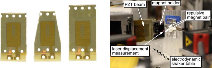
Figure 8. (a) Three beams shapes for experiments. (b) Photograph of the experiment platform.
Table 4. Parameters for three beams identified from experiments.
d2 (mm)
L (mm) bL (mm) hs (mm) hc (mm) Monostable case Bistable case e33 (nF m−1) e31 (C m−2) M0 (g)
Beam 1 37.4 32 0.034 0.02 10.8 10.4 30.15 −14.54 16.6
Beam 2 37.4 18 0.04 0.02 10.6 10.3 30.15 −14.54 16.6
Beam 3 45 32 0.034 0.02 11.8 11.6 30.15 −14.54 7.0
beam axis, as shown in figure 8(b). The shaker table is driven by monostable configuration. Figures 9(d) and (e) are the
a controller (Vibration Research Controller VR9500) and corresponding responses for a bistable configuration of each
amplifier (Crown XLS 2500) with an accelerometer (PCB Pie- beam. Analytical predictions are shown as the thick curves
zotronics 333B40) to provide control signal feedback to ensure whereas the experimental results are presented using thin
the base acceleration amplitude remains 5 m s−2 at all fre- curves in the same respective line style. Because the strain at
quencies examined. Two laser displacement sensors (Micro- the clamped ends of the beams cannot be measured without
Epsilon ILD-1420) measure the absolute displacement of the influencing the laminated beam mechanical properties, the
beam tip and the shaker table. A bridge rectifier (1N4148 strain responses shown in figures 9(c) and (f) are calculated
diodes) with a smoothing capacitor Cr and resistive load R are from finite element analysis (FEA) using ABAQUS. In the
connected to the piezoelectric beam to quantify the converted FEA, a solid model of the exact beam composition is used,
electric energy. where all parameters employed are provided in tables 2 and 4.
Rigid elements are included to model the aluminum magnet
6. Experiment validation holder, and a mass element is used to model the beam tip
mass. After establishing the finite element model, the dis-
The experiments examine both monostable and bistable placement amplitudes shown in figures 9(a) and (d) are
configurations of beams 1, 2, and 3. Figures 9(a) and (b) applied as boundary conditions for the FEA to compute a
respectively show the displacement amplitude of the beam tip static load analysis that provides values of the clamped end
and rectified output voltage of the three beams for a strain, using the strain at the middle of the clamp.
13Smart Mater. Struct. 28 (2019) 075040 W Cai and R L Harne
Figure 9. Frequency responses for three beams. (a) Displacement amplitude at the beam tip, (b) rectified output voltage, and (c) strain at the
fixed end for monostable configurations. (d)–(f) Corresponding responses for bistable configuration.
Figure 10. Comparison of cost function values between experiment and analysis for three beam designs. (a) Frequency range. (b) Total RMS
of the rectified output voltage. (c) Total RMS of the strain at the fixed end.
From the displacement responses shown in figures 9(a) and electromechanical behaviors of the piezoelectric laminated
(d), the large displacement amplitudes at the bifurcations are in energy harvester.
good agreement between the analysis and experimentation. The results of figure 10 establish the efficacy of the
Since the stiffness of the beam is increased due to the rigid cross- optimization created through this research. The results of
section assumption in Euler–Bernoulli beam theory, the analy- monostable cases of all three beams suggest a higher output
tical strain predictions in figures 9(c) and (f) are relatively greater voltage with a lower strain level and a wider frequency range
than the FEA results using the experimental data of displacement (red or blue bars) when compared to the bistable configurations
amplitude. This in turn increases the predicted analytical output of the energy harvesters (green or cyan bars). This emphasizes
voltage in figures 9(b) and (e) compared to the experimental the global superiority of monostable platforms over bistable
levels. Electrical component losses and higher order harmonics system configurations to achieve broadly robust energy har-
are also neglected in analysis, which may also contribute to vesting performance and agrees with results obtained
the overprediction of rectified voltage. The grey shaded areas throughout section 4. In addition, the tapered beam 2 exhibits
in figures 9(d)–(f) correspond to multi-harmonic or chaotic quantitatively less strain at the clamped end than the rectan-
dynamic behaviors that are not predicted by analysis due gular beam 1 of the same length, figure 10(c), while the beam 2
to steady-state assumptions in the solution formulation. is within 1 V RMS of the rectified output voltage of beam 1,
Despite these discrepancies, the overall quantitative agreement figure 10(b). This result agrees with the findings of
between the experimental and analytical results in figure 9 section 4.2.2. Furthermore, when the tip mass decreases to 7 g
exemplifies that the model formulation accurately replicates the for beam 3, the frequency range may still be broad by
14Smart Mater. Struct. 28 (2019) 075040 W Cai and R L Harne
introducing sufficient nonlinearity as shown in figure 10(a). 2014 Int. Symp. on Low Power Electronics and Design (La
Yet, the output voltage and strain for beam 3 in figures 10(b) Jolla) pp 375–80
and (c) are decreased comparing with the results of the other [4] Gorlatova M, Sarik J, Grebla G, Cong M, Kymissis I and
Zussman G 2014 Movers and shakers: kinetic energy
two beams, which supports the influences uncovered in harvesting for the Internet of things ACM SIGMETRICS
section 4.2.3. Thus, considering the design constraints exam- Perform. Eval. Rev. 42 407–19
ined here, piezoelectric laminated cantilevers with tapered [5] Cho J, Anderson M, Richards R, Bahr D and Richards C 2005
shapes, monostable nonlinearity, and moderate lengths deliver Optimization of electromechanical coupling for a thin-film
the most performance robust DC power delivery. PZT membrane: I. Modeling J. Micromech. Microeng.
15 1797
[6] Wang Q and Wu N 2012 Optimal design of a piezoelectric
coupled beam for power harvesting Smart Mater. Struct. 21
7. Conclusions 085013
[7] Lü C, Zhang Y, Zhang H, Zhang Z, Shen M and Chen Y 2019
This research provides the first illumination of the coupled Generalized optimization method for energy conversion and
storage efficiency of nanoscale flexible piezoelectric energy
influences of nonlinearity and beam shape design on the harvesters Energy Convers. Manage. 182 34–40
resulting mechanical robustness and versatile electrical power [8] Qin L, Jia J, Choi M and Uchino K 2019 Improvement of
generation of a nonlinear energy harvesting system. Here, an electromechanical coupling coefficient in shear-mode of
analytical model is established and verified through numerical piezoelectric ceramics Ceram. Int. 45 1496–502
simulations and experimental examinations for key influences [9] Baker J, Roundy S and Wright P 2005 Alternative geometries
for increasing power density in vibration energy scavenging
of nonlinearity, beam shape, and tip mass select result in robust for wireless sensor networks 3rd Int. Energy Conversion
system designs. Multi-objective optimization guides attention to Engineering Conf. (San Francisco) pp 2005–5617
strategic combinations of design parameters based on the spe- [10] Hosseini R and Hamedi M 2015 Improvements in energy
cific optimization variables and relative weights given to the harvesting capabilities by using different shapes of
objective functions. Trapezoidal beam shapes are found to piezoelectric bimorphs J. Micromech. Microeng. 25 125008
[11] Roundy S et al 2005 Improving power output for vibration-
promote large output voltage without yielding high strain at the based energy scavengers IEEE Pervasive Comput. 1 28–36
clamped end, which promotes practical longevity of the system. [12] Montazer B and Sarma U 2018 Design and optimization of
Bistable implementations of the nonlinear energy harvesters are quadrilateral shaped PVDF cantilever for efficient
found to be undesirable for sake of large residual strain at the conversion of energy from ambient vibration IEEE Sens. J.
clamped end, even though they may deliver wide frequency 18 3977–88
[13] Tabatabaei S M K, Behbahani S and Rajaeipour P 2016 Multi-
range of operation and high output voltages. Therefore, both the objective shape design optimization of piezoelectric energy
optimization results using the new analysis and experiment harvester using artificial immune system Microsyst. Technol.
validations indicate that a trapezoidal beam in a monostable 22 2435–46
configuration is globally preferred. [14] Matova S P, Renaud M, Jambunathan M, Goedbloed M and
Van Schaijk R 2013 Effect of length/width ratio of tapered
beams on the performance of piezoelectric energy harvesters
Smart Mater. Struct. 22 075015
Acknowledgments [15] Dietl J M and Garcia E 2010 Beam shape optimization for
power harvesting J. Intell. Mater. Syst. Struct. 21 633–46
This research is supported by the National Science Founda- [16] Raju S S, Umapathy M and Uma G 2018 High-output
tion under Award No. 1661572. The authors are grateful to piezoelectric energy harvester using tapered beam with
cavity J. Intell. Mater. Syst. Struct. 29 800–15
hardware support from Midé Technology. [17] Xu J W, Liu Y B, Shao W W and Feng Z 2012 Optimization of
a right-angle piezoelectric cantilever using auxiliary beams
with different stiffness levels for vibration energy harvesting
ORCID iDs Smart Mater. Struct. 21 065017
[18] Yoon H S, Washington G and Danak A 2005 Modeling,
optimization, and design of efficient initially curved
Wen Cai https://orcid.org/0000-0002-7274-9884 piezoceramic unimorphs for energy harvesting applications
Ryan L Harne https://orcid.org/0000-0003-3124-9258 J. Intell. Mater. Syst. Struct. 16 877–88
[19] Chandrasekharan N and Thompson L L 2016 Increased power
to weight ratio of piezoelectric energy harvesters through
References integration of cellular honeycomb structures Smart Mater.
Struct. 25 045019
[20] Harne R L and Wang K W 2017 Harnessing Bistable
[1] Magno M, Spadaro L, Singh J and Benini L 2016 Kinetic Structural Dynamics: for Vibration Control, Energy
energy harvesting: toward autonomous wearable sensing for Harvesting and Sensing (Chichester: Wiley)
internet of things 2016 Int. Symp. on Power Electronics, [21] Cottone F, Vocca H and Gammaitoni L 2009 Nonlinear energy
Electrical Drives, Automation and Motion (Anacapri) harvesting Phys. Rev. Lett. 102 080601
pp 248–54 [22] Harne R L and Wang K W 2013 A review of the recent
[2] Evans D 2011 The internet of things: how the next evolution of research on vibration energy harvesting via bistable systems
the internet is changing everything CISCO White Pap. 1 Smart Mater. Struct. 22 023001
1–11 [23] Erturk A, Hoffmann J and Inman D J 2009 A
[3] Jayakumar H, Lee K, Lee W S, Raha A, Kim Y and piezomagnetoelastic structure for broadband vibration
Raghunathan V 2014 Powering the internet of things Proc. energy harvesting Appl. Phys. Lett. 94 254102
15You can also read