Lawrence Berkeley National Laboratory - Recent Work

Lawrence Berkeley National Laboratory
Recent Work

Title
Implausible projections overestimate near-term Bitcoin CO2 emissions

Permalink
https://escholarship.org/uc/item/8vf573nb

Authors
Masanet, E
Shehabi, A
Lei, N
et al.

Publication Date
2019-09-01

DOI
10.1038/s41558-019-0535-4

Peer reviewed

 eScholarship.org Powered by the California Digital Library
 University of California

LBNL-2001235

Implausible projections overestimate near-
term Bitcoin CO2 emissions
Authors:
Eric Masanet1,2, Arman Shehabi3, Nuoa Lei1, Harald Vranken4, Jonathan Koomey5
and Jens Malmodin6
1
 Department of Mechanical Engineering, Northwestern University
2
 Department of Chemical and Biological Engineering, Northwestern University
3
 Energy Analysis & Environmental Impacts Division, Lawrence Berkeley National Laboratory
4
 Faculty of Management, Science & Technology, Open University of the Netherlands & Radbound University
5
 Special Advisor to the chief Scientist of Rocky Mountain Institute
6
 Ericsson

Energy Analysis and Environmental Impacts Division
Lawrence Berkeley National Laboratory

September/2019

 This material includes work conducted by Lawrence Berkeley National Laboratory with support from the
 Department of Energy Advanced Manufacturing Office. Lawrence Berkeley National Laboratory is supported
 by the Office of Science of the United States Department of Energy and operated under Contract Grant No.
 DE-AC02-05CH11231.

DISCLAIMER

This document was prepared as an account of work sponsored by the United States Government. While this
document is believed to contain correct information, neither the United States Government nor any agency thereof,
nor The Regents of the University of California, nor any of their employees, makes any warranty, express or implied,
or assumes any legal responsibility for the accuracy, completeness, or usefulness of any information, apparatus,
product, or process disclosed, or represents that its use would not infringe privately owned rights. Reference herein
to any specific commercial product, process, or service by its trade name, trademark, manufacturer, or otherwise,
does not necessarily constitute or imply its endorsement, recommendation, or favoring by the United States
Government or any agency thereof, or The Regents of the University of California. The views and opinions of authors
expressed herein do not necessarily state or reflect those of the United States Government or any agency thereof,
or The Regents of the University of California.

Ernest Orlando Lawrence Berkeley National Laboratory is an equal opportunity employer.

 COPYRIGHT NOTICE

This manuscript has been authored by an author at Lawrence Berkeley National Laboratory under Contract No.
DE-AC02-05CH11231 with the U.S. Department of Energy. The U.S. Government retains, and the publisher, by
accepting the article for publication, acknowledges, that the U.S. Government retains a non-exclusive, paid-up,
irrevocable, worldwide license to publish or reproduce the published form of this manuscript, or allow others to
do so, for U.S. Government purposes.

Implausible projections overestimate near-term Bitcoin CO2 emissions
Eric Masanet1,2*, Arman Shehabi3, Nuoa Lei1, Harald Vranken4, Jonathan Koomey5, and Jens Malmodin6
 1
 Department of Mechanical Engineering, Northwestern University
 2
 Department of Chemical and Biological Engineering, Northwestern University
 3
 Energy Analysis & Environmental Impacts Division, Lawrence Berkeley National Laboratory
 4
 Faculty of Management, Science & Technology, Open University of the Netherlands & Radboud
 University
 5
 Special Advisor to the Chief Scientist of Rocky Mountain Institute
 6
 Ericsson

 * email: eric.masanet@northwestern.edu

Author contributions

All authors contributed equally to the conception and design of this critique, and to the preparation and
review of the manuscript. Masanet, Shehabi, Lei, and Vranken led the analytical components of this
critique.

Competing interests

The authors declare no competing financial or non-financial interests.

Data availability

The authors declare that all data supporting the findings of this critique are available within the article,
its Supplementary Information file and at https://github.com/emasanet/Bitcoin-analysis.

Bitcoin mining is becoming an increasingly energy-intensive process1,2,3 whose future implications for
energy use and CO2 emissions remain poorly understood. This is in part because—like many IT
systems—its computational efficiencies and service demands have been evolving rapidly. Therefore,
scenario analyses that explore these implications can fill pressing knowledge gaps, but they must be
approached with care. History has shown that poorly constructed scenarios of future IT energy use—
often due to overly-simplistic extrapolations of early rapid growth trends—can do more harm than good
by spreading misinformation and driving ill-informed decisions.4,5,6 Indeed, the utility of an energy
demand scenario is directly proportional to its credibility, which is typically demonstrated through
careful attention to technology characteristics and evolution, analytical rigor and transparency, and
designing scenarios that align with plausible future outcomes.

Regrettably, the Bitcoin CO2 emissions scenarios presented in the recent Mora et al. article7 lack such
credibility and should not be taken seriously by the research and policy communities. We arrived at this
conclusion by replicating in detail Mora et al.’s methods, which revealed numerous flaws in the design
and execution of their analysis as documented in the Supplementary Information. We describe the five
most significant issues below.

First, the use of transactions as the driver of future Bitcoin emissions is questionable, given the tenuous
correlation between transactions and mining energy use. It is well established that energy use is driven
by the computational difficulty of blocks mined1-3, whereas the number of transactions per block has no
effect on block mining difficulty. Indeed, the authors themselves calculate 2017 Bitcoin energy use and
emissions based on block difficulty, not number of transactions (Supplementary Eq. 1). Without
explanation or justification, the authors switch to transactions as the driver for projecting emissions in
all future years, undermining the consistency of their calculations and the integrity of their projections.

Second, all three Bitcoin adoption scenarios designed by Mora et al. represent sudden and highly
improbable departures from historical trends in Bitcoin transactions, whose annual growth ranged from
1.3x-2.3x over the preceding five years.8 Specifically, Mora et al. assume that Bitcoin transactions—
which totaled 104 million in 2017, representing a mere 0.03% of global cashless transactions—would
abruptly leap to 78 billion by 2019 in the fast scenario (a 750x increase in only 2 years), to 11 billion by
2020 in the median scenario (a 108x increase), and to 8 billion by 2023 in the slow scenario (a 76x
increase). All three adoption scenarios follow steep logarithmic growth trajectories thereafter, which
are conspicuously inconsistent with historical trends (Supplementary Fig 4), and which mathematically
can only lead to large near-term emissions increases. The authors base their scenarios on adoption rates

of 40 “broadly used” technologies whose social utilities vary widely and bear little resemblance to that
of Bitcoin. The authors never explain why such comparisons are valid, nor do they justify the plausibility
of the very abrupt changes in Bitcoin transaction levels and growth trajectories associated with their
resulting scenarios. Hence, these scenarios should not be taken seriously.

Third, Mora et al. applied outdated values for mining rig efficiencies and electric power carbon
intensities, which inflated their estimated 2017 Bitcoin energy use and CO2 emissions values
considerably. When estimating the direct electricity use of Bitcoin mining, the authors erroneously
included many old and inefficient rigs in their selection pool that were no longer economically viable in
2017 (Supplementary Fig 5), betraying a lack of understanding of current mining equipment and
economics. Furthermore, Mora et al provided equal weighting when selecting a rig from their pool as
the sole rig type to mine a block, thus over-representing slower inefficient rigs and creating scenarios
that require physically impossible rig counts. When we excluded unprofitable rigs in our replicated
analysis, Mora et al.’s model produced an estimate of 28 TWh in 2017 (Supplementary Fig 6), which is
one fourth of their original estimate of 114 TWh. Furthermore, they applied 2014 carbon intensities (g
CO2/kWh) to calculate 2017 emissions, ignoring non-negligible grid decarbonization improvements in
the intervening years (Supplementary Fig 7),9 even though sufficient data existed at the time of their
study for reasonable estimates of 2017 carbon intensities.10,11 Applying more reasonable 2017
electricity use and carbon intensity values in their model produced an estimate of 15.7 MtCO2e, far
lower than their original estimate of 69 MtCO2e.

Fourth, by analytical design, Mora et al. applied 2017 per-transaction energy use and CO2 emissions
values in all future years, multiplied by annual transactions (Supplementary Eq 2). This decision
effectively held both mining rig efficiency and grid carbon intensities constant for the next 100 years
(Supplementary Fig 7). This dubious choice ignores the dynamic natures of mining rig and power grid
technologies and violates the widely-followed practice of accounting for technological change in
forward-looking energy technology scenarios. In acknowledging their static grid intensity assumption,
they point to at least one reference containing credible grid intensity outlooks10 but failed to utilize
them. Estimating the future energy efficiency of mining is certainly difficult, but the authors never
explain why they simply ignored this important scenario consideration, nor do they justify how assuming
static mining efficiency for 100 years—when mining rigs have evolved monthly1— can lead to any useful
insights.

Fifth, in constructing their slow, median, and fast adoption scenarios, Mora et al. committed key errors
when analyzing adoption rates within their 40-product comparison pool.12 Namely, when replicating
their analysis, we discovered that, for many comparison products, they designated the first available
data point as the first year of product usage. For example, the authors designate the first year of usage
for electric power as 1908, at which point U.S. household adoption had climbed to 10% (Mora et al. Fig.
1b). Yet Thomas Edison began offering electric power to (far fewer) U.S. households in Manhattan in
1882, over two decades earlier.13 By omitting the initial low-adoption years of US market availability for
numerous technologies, their scenarios were biased toward inaccurately steep near-term adoption
trajectories in all three cases. When we replicated their analysis using more reasonable estimates of the
first year of technology usage, their own methods produced slower adoption curves, particularly in the
median and slow growth scenarios (Supplementary Fig 8).

To assess how these last three analytical flaws affected Mora et al.’s projections, we replicated their
original scenario analysis (Fig 1a), and then applied reasonable corrections in stepwise fashion. We first
applied the 2017 per-transaction Bitcoin carbon intensity we obtained by excluding unprofitable rigs (Fig
1b). We then utilized weighted-average grid intensities based on mining locations assumed by the
authors, including grid intensity evolution based on IEA outlooks that reflect current and announced
national power policies in mining locations (Supplementary Fig 7) (Fig 1c). Finally, we applied our
calculated adoption curves in all three scenarios (Fig 1d).

The results show that, had the authors avoided the key errors we described above, their own study
design would have yielded much different, and far less alarming, projections of future Bitcoin carbon
emissions. That said, we find the study design itself sufficiently flawed—e.g., use of transactions as
driver, comparisons to 40 unrelated technologies, ignoring rig evolution—that such corrections alone
are not enough to salvage the authors’ approach. On these bases, we argue that the Mora et al.
scenarios are fundamentally flawed and should not be taken seriously by researchers, policymakers, or
the public.

Given the highly dynamic and unpredictable nature of Bitcoin markets and mining demand—e.g., Bitcoin
transactions and exchange values dropped steeply in 2018—developing credible scenarios of
cryptocurrency emissions remains an important challenge for the research community. While Mora et
al. likely had the right motivations, to be useful, such scenarios must be approached with more rigor and
greater analytical care.

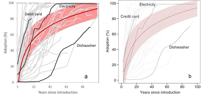
Figure 1: Comparison of Bitcoin CO2 emissions projected by the Mora et al. model: (a) our replicated
analysis showing close agreement with the authors’ results; and the model’s projections after first (b)
removing unprofitable rigs in the base year (median scenario only), then (c) accounting for evolution
of the electric power grid in mining locations (median scenario only), and finally (d) correcting errors
in their stated adoption scenario approach.

References

1
 Vranken, H. Sustainability of bitcoin and blockchains. Current Opinion in Environmental Sustainability
28, 1-9, doi:https://doi.org/10.1016/j.cosust.2017.04.011 (2017).

2
 Krause, M. J. & Tolaymat, T. Quantification of energy and carbon costs for mining cryptocurrencies.
Nature Sustainability 1, 711-718, doi:10.1038/s41893-018-0152-7 (2018).

3
 Bevand, M. Op Ed: Bitcoin Miners Consume A Reasonable Amount of Energy — And It's All Worth It,
 (2017).

4
 Koomey, Jonathan G, Chris Calwell, John A Laitner, Jane Thornton, Richard E Brown, Joseph H Eto,
Carrie A Webber, and Cathy Cullicott. "Sorry, wrong number: The use and misuse of numerical facts in
analysis and media reporting of energy issues." Ed. Socolow, Robert H, Dennis Anderson, and John
Harte. Annual Review of Energy and the Environment 2002 27 (2002) 119-158. LBNL-50499.
5
 Koomey, Jonathan, Huimin Chong, Woonsien Loh, Bruce Nordman, and Michele Blazek. 2004.
"Network electricity use associated with wireless personal digital assistants." The ASCE Journal of
Infrastructure Systems (also LBNL-54105). vol. 10, no. 3. September. pp. 131-137.
[http://ascelibrary.org/doi/abs/10.1061/(ASCE)1076-0342(2004)10%3A3(130)]
6
 Koomey, J. Turning Numbers into Knowledge: Mastering the Art of Problem Solving. (Analytics Press,
2017).

7
 Camilo Mora, Randi L. Rollins, Katie Taladay, Michael B. Kantar, Mason K. Chock, Mio Shimada & Erik C.
Franklin. Bitcoin emissions alone could push global warming above 2°C. Nature Climate Changevolume
8, pages931–933 (2018)
8
 Bitcoinity. Number of transactions - Bitcoinity.org. (2019).
http://data.bitcoinity.org/bitcoin/tx_count/5y?t=l

9
 International Energy Agency. Power - Tracking Clean Energy Progress. (IEA, 2019).
https://www.iea.org/tcep/power/

10
 International Energy Agency. Energy Technology Perspectives 2017. (IEA, 2017).

11
 International Energy Agency. World Energy Outlook 2017. (IEA, 2017).

12
 Our World in Data. Technology adoption by households in the United States. (2019).
https://ourworldindata.org/grapher/technology-adoption-by-households-in-the-united-
states?time=1903..2016

13
 Ania Monaco. Edison's Pearl Street Station Recognized With Milestone: IEEE honors the world's first
central power station. 27 July 2011. (2011). http://theinstitute.ieee.org/tech-history/technology-
history/edisons-pearl-street-station-recognized-with-milestone810

Supplementary Information
Implausible projections overestimate near-term Bitcoin CO2 emissions
Eric Masanet1,2*, Arman Shehabi3, Nuoa Lei1, Harald Vranken4, Jonathan Koomey5, and Jens Malmodin6
 1
 Department of Mechanical Engineering, Northwestern University
 2
 Department of Chemical and Biological Engineering, Northwestern University
 3
 Energy Analysis & Environmental Impacts Division, Lawrence Berkeley National Laboratory
 4
 Faculty of Management, Science & Technology, Open University of the Netherlands & Radboud
 University
 5
 Special Advisor to the Chief Scientist of Rocky Mountain Institute
 6
 Ericsson

 * email: eric.masanet@northwestern.edu

In this document we show that the analysis by Mora et al., which predicts that Bitcoin mining alone can
increase global warming by more than 2 C in 11 to 22 years, is fundamentally flawed and should not be
taken seriously by researchers, policymakers, or the general public.

Hereafter we refer to Mora et al. as “the authors.” We first document our replication of the authors’
original methods and results in Sections I, II, and III, elaborating on several methodological problems we
encountered during the process. Next, in Sections IV-VIII, we discuss in depth five major flaws related to
the authors’ study design and execution. As part of these discussions, we apply our replicated model to
demonstrate that, had the authors avoided some key analytical errors, their own model would have
produced significantly lower carbon emissions trajectories that invalidate their original alarmist
predictions.

 I. Replication of 2017 CO2 emissions estimate

We first replicated the authors’ 2017 Bitcoin CO2 emissions estimate, based on the R script they
provided as their model. We generalize their calculation approach as follows (using our own notation):
 
 2017 = ∑ =1 3.6∗10
 
 6 (1)

The variable C2017 is Bitcoin’s global carbon emissions quantity in 2017, expressed in units of grams of
CO2 equivalents (g CO2e). Ei is the energy efficiency of the mining rig assigned to solve block i, expressed
in units of joules of direct electricity use per hash (J/H). The authors assign rigs randomly (i.e., with equal
probability) to each block from a list they provide in their Supplementary Information (SI) Table 1. Hi is
the expected number of hashes required to solve block i, which is calculated by multiplying its difficulty
by 232. Gi is the regional CO2 intensity of grid electricity generation (g CO2e/kWh), which the authors
assign depending on which pool solved block I as documented in their SI Table 2. The denominator

 1

converts direct electricity use from joules into kWh (1 kWh = 3.6*106 joules). The results are summed
over n = 55,864 blocks, the total number solved in 2017.

Our replication of the authors’ code generated an expected 2017 global Bitcoin CO2 emissions value
(C2017) of 69 Mt CO2e (18.8 Mt C), which is identical to the authors’ result, and an expected 2017 global
Bitcoin direct electricity use value of 114 TWh. The latter value was not reported by the authors.

 II. Replication of future CO2 emissions projections

Next we attempted to replicate the authors’ future projections of Bitcoin CO2 emissions. The authors did
not provide code or explicit formulae for replicating their projections. Therefore, we had to rely on the
authors’ qualitative methodological descriptions and their results graphs to generalize their projection
approach mathematically as follows (using our own notation):

 = 2017 ̂2017 (2)

The variable Cj is Bitcoin’s global CO2 emissions quantity in future year j (g CO2e). T2017 is the total
number of global cashless transactions in 2017 (314.2 billion), which the authors assume will remain
constant for all future years j. The variable fj is the authors’ assumed fraction of global cashless
transactions attributable to Bitcoin in year j. Ĉ2017 is Bitcoin’s average per-transaction carbon emissions
intensity (g CO2e/transaction) associated with solving all blocks in 2017.

We note that the authors calculate Cj each year by randomly selecting combinations of blocks that had
already been solved in their estimation of 2017 Bitcoin CO2 emissions (as described in Section I) until
total Bitcoin transactions in year j are fulfilled. This procedure is repeated 1,000 times. This approach
effectively delivers an expected per-transaction CO2 intensity in each year j that is very similar to the
simple quotient of 2017 expected carbon emissions (69 Mt CO2e) and 2017 total Bitcoin transactions
(103.7 million). This quotient has a value of Ĉ2017 = 665 kg CO2e/trans (181 kg C/trans).

Therefore, we use this constant Ĉ2017 value for analytical efficiency in our results replication, given that
the authors use transactions as their future emissions driver (i.e., activity variable) in Eq. 2. In doing so,
we arrive at very similar CO2 emission projections to those of the authors, as discussed below.

The authors construct three different scenarios for fj, which they provide over a 100-year projection
period, based on their adoption rate analysis of 40 different “broadly adopted” technologies. Our
replication of the authors’ Bitcoin CO2 emissions projections, which were generated using Eqs. (1) and
(2) and the authors’ values for fj, are shown in Supplementary Fig. 1.

Before comparing our replicated results to those of the authors, three caveats are required:

 1. The authors’ lack of transparency prevents precise comparisons. The authors did not provide
 their numerical projection results; instead, they only provided one projection results figure with
 coarse axis scales (their Fig. 1c). This lack of transparency makes exact replication impossible.
 Therefore, we checked the general accuracy of our replication by comparing our results to their
 Figure 1c and to the number of years stated by the authors until cumulative Bitcoin CO2
 emissions would exceed 231.4 Gt C (the authors’ lower 2 C warming threshold).

 2. The authors’ base year, and its associated cumulative CO2 emissions, are unclear. Without
 explanation or explicit acknowledgement, the authors appear to have chosen 2020 as the base

 2

year for projections in their Fig. 1c, even though they had earlier estimated 2017 Bitcoin CO2
 emissions. Furthermore, and again without explanation, the authors appear to have assumed a
 cumulative global anthropogenic CO2 emissions value of around 585 Gt C in 2020 (which we
 estimated via direct measurement of Fig. 1c), to which they cumulatively add projected Bitcoin
 CO2 emissions over time in each scenario. Yet, in their paper, the authors also state that
 cumulative global anthropogenic carbon emissions had already reached 584.4 Gt C in 2014, six
 years earlier. This is a glaring analytical inconsistency that we could not reconcile when
 replicating the authors’ projections.

 3. The authors’ Bitcoin adoption values are opaquely labeled and incongruous. We encountered
 several difficulties interpreting the authors’ data for Bitcoin adoption (fj), which they provided in
 a downloadable file for three different scenarios: median, lower25, and upper75. These three
 scenarios are represented in the paper as typical, slow, and fast adoption pathways,
 respectively. The authors label the year of each adoption value (fj) ordinally, starting with a
 value of 2, while their emissions projection results are labeled by calendar year starting in 2020.
 They do not explain which ordinal year corresponds to which calendar year in their results, nor
 do they provide an ordinal year 1. Furthermore, the authors provide several negative values of
 Bitcoin adoption (fj)—specifically, for ordinal year 2 in the median scenario and for ordinal years
 2-5 in the lower25 scenario—which are physical impossibilities and incongruous with current
 (albeit small) Bitcoin adoption levels. They do not explain these negative adoption values, which
 are also clearly visible in their Fig 1b, which appears to start in ordinal year 2. In light of these
 documentation deficiencies, we attempted to establish correspondence between their Figs 1b
 and 1c (via Eqs 1 and 2) and concluded that the authors most likely assigned ordinal year 3 to
 calendar year 2020 in their analysis and simply ignored years with negative Bitcoin adoption
 values in each scenario, even though Bitcoin currently has a positive (albeit small) market
 penetration and will continue emitting CO2 until 2020 in any scenario. The authors’ failure to
 provide numerical results and explanations of ordinal years and negative values make it
 impossible to verify our conclusions about the authors’ intentions in these figures. However,
 these conclusions do enable us to replicate the authors’ results quite accurately.

With these caveats in mind, our replicated results in Supplementary Fig. 1 show similar carbon emissions
trajectories for all three scenarios compared to the authors’ Fig 1c. Our results also replicate the
authors’ calculations indicating that cumulative Bitcoin CO2 emissions cross the 231.4 Gt C threshold in
2028, 2033, and 2039 in the Upper75, median, and Lower25 scenarios, respectively. However, the
aforementioned methodological issues already raise serious questions about the credibility of the
authors’ analysis.

 3

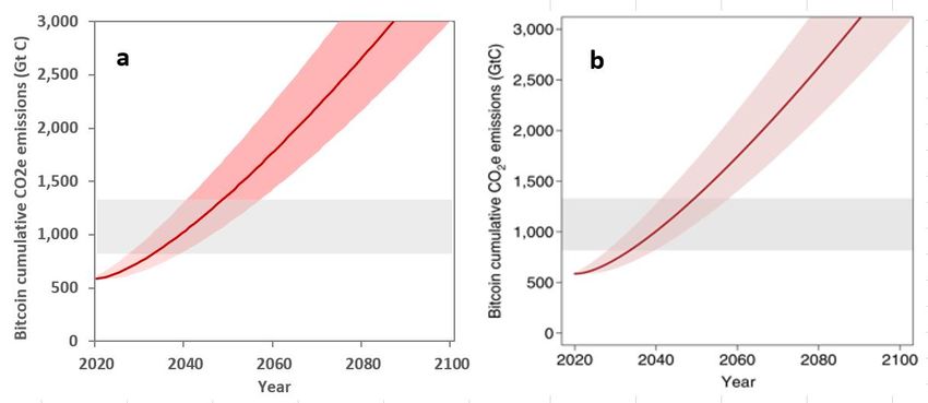
Supplementary Figure 1. (a) Our replicated Bitcoin CO2 emissions projections using the authors’ data
and model; (b) the authors’ Bitcoin CO2 emissions projections, as shown in their Figure 1c.

 III. Replication of Bitcoin adoption scenarios

To better understand the basis for the authors’ steep growth trajectories in all three scenarios they
considered, we also replicated their derivation of Bitcoin adoption values in each scenario based on
their stated comparison to 40 “broadly adopted” technologies. To do so, we obtained the same source
data used by the authors1,2 and replicated their comparative analysis, first by normalizing all adoption
data in the same manner as the authors, then by constructing regression curves for the median, 25th
percentile, and 75th percentile of the technology adoption ranges each year. Our replicated median,
lower25, and upper75 adoption curves are shown in Supplementary Fig. 2, which are in close agreement
with those of the authors in their Fig 1b (repeated below for convenience).

Our replication also revealed a likely error in the authors’ representation of data contained in their Fig.
1b. Namely, the rapidly rising trendline labeled “credit card” appears to be based on adoption data for
debit cards in the original source2, not credit cards.

This error is notable, in that many readers of the Mora et al. paper may look to credit cards as the most
appealing comparison product among the 40 in the authors’ pool—given that early credit cards
represented a disruptive new transaction technology—and form opinions about Bitcoin’s future
adoption potential on this basis. However, credit card usage in the United States followed a more
gradual adoption path than that shown in the authors’ Fig. 1b. Specifically, the first universal U.S. credit
card (Diner’s Club) was introduced in 19503 and by 1970 (20 years later) the fraction of U.S. families
holding credit cards had risen to 50%4, whereas the authors’ (mislabeled) adoption curve implies that
credit cards grew much faster, penetrating around 80% of U.S. households in a similar time period.

 4

Supplementary Figure 2. (a) Our replication of the authors’ Bitcoin adoption scenarios; (b) the
authors’ original Bitcoin adoption scenarios as shown in their Figure 1b.

Next, we discuss two major study design flaws that became apparent to us during the process of
replicating Mora et al.’s methods and results.

 IV. The use of transactions as an energy demand driver is questionable

As summarized in Eq. 2, the authors project Bitcoin’s future CO2 emissions in each scenario using
transactions as the emissions driver—i.e., the activity variable— in all future years. We consider this
approach as a fundamental study design flaw, since it is well known that the electricity consumed, and
hence the CO2 emitted, by Bitcoin mining does not depend on the number of transactions but, rather,
on the difficulty and number of blocks mined. 5,6,7

The pace at which blocks are mined is kept constant at around 6 blocks per hour. The difficulty
parameter in the mining algorithm is adjusted every 14 days to maintain this pace. An increasing
number of transactions will therefore not cause an increase in the number of blocks. Instead, this will
cause that individual blocks will include more transactions. The effort to mine a block is however
independent of the number of transactions in the block.

Indeed, the authors themselves calculate 2017 Bitcoin energy use and emissions based on block
difficulty, not number of transactions (Eq. 1). Without explanation or justification, the authors switch to
transactions as the driver for projecting emissions in all future years, undermining the consistency of
their calculations and the integrity of their projections.

To illustrate this flaw, let’s assume that all 314.2 billion cashless transactions in 2017 would be Bitcoin
transactions. Then in the authors’ approach this takes about 159 million blocks (considering that one
block contained on average about 1,974 transactions in 2017).8 This implies mining at a pace of 18,170
blocks per hour—three orders of magnitude greater than the established fixed pace of 6 blocks per
hour—which betrays a lack of understanding of how real-world mining works. In contrast, in the above
example, transactions would be increased on average to 5,977,930 per block, keeping the pace nearly

 5

constant at 6 blocks mined per hour. Hence, blocks will become much larger, which will cause scalability
issues, mainly in communication latency, but it would not necessarily increase mining effort.

 V. The authors’ Bitcoin adoption scenarios are implausible

As evident in Eq. (2), the authors’ future Bitcoin CO2 emissions estimates are sensitive to their design of
adoption scenarios (fi). The authors’ typical, slow, and fast adoption scenarios are plotted in
Supplementary Fig 1b, which paints a seemingly unavoidable future of sudden and rapid Bitcoin
adoption. Mathematically, the authors’ use of steep logarithmic growth curves in all scenarios can only
result (see Eq. 2) in large near-term increases in Bitcoin’s carbon emissions, even in the slowest adoption
scenario.

The authors implicitly justify steep future growth by pointing to rapid historical (2009-2017) growth in
global Bitcoin transactions (the authors’ Supplementary Figure 1), which they model using a power
function. However, 2018 data (most of which were available prior to publication of the authors’ study)
expose the well-documented danger of simply extrapolating past trends into the future: global Bitcoin
transactions fell by 22% in 20189. Therefore, in 2018, as shown in Supplementary Fig. 3, the authors’
power model already overestimates global Bitcoin transactions by a factor of 2. This discrepancy
underscores why readers should be wary of any future energy/carbon emission projections based on
simple extrapolation of early rapid growth trends, especially for information technology (IT) systems,
whose efficiencies and service demands can evolve quickly. 10,11,12

Supplementary Figure 3. Annual global Bitcoin transactions (2009-2018) with the authors’ historical
(2009-2017) power model extended to 2018.

 6

Upon initial observation, the steep upward slope of the authors’ historical power model (Supplementary
Fig. 3) might seem visually coherent with the steep initial upward slopes of the authors’ future adoption
scenarios (authors’ Fig 1b). However, when these data series are plotted together on the same scale—
i.e., billions of transactions—major inconsistencies emerge. As shown in Supplementary Fig. 4, the
authors’ own historical power model follows a much flatter future trajectory in the near-term compared
to the Bitcoin transactions assumed by the authors in their scenarios, all three of which abruptly switch
to significantly steeper trajectories at their outsets.

Supplementary Figure 4. Comparison of historical (2009-2017) Bitcoin transactions and the future
Bitcoin transactions associated with the authors’ power model and their three adoption scenarios.
Note: Due to negative initial values and missing data for 2018 (see Section II), the authors’ three
scenarios have different start years and are represented here with different styles than in previous
graphs for clarity.

Moreover, in the first year of each of the authors’ scenarios, implausibly massive jumps in Bitcoin
transactions would be required to bridge the gaps compared to present-day totals. In 2017, global
Bitcoin transactions totaled 104 million, or a mere 0.03% of global cashless transactions.13 In the
authors’ scenarios, however, the following must happen:

  by 2019 (i.e., only 2 years later), Bitcoin adoption must jump to:
 o 78 billion transactions in the fast scenario, which represents a:
  750x increase compared to 2017, and a
  280x increase compared to their power model extrapolated to 2019
  by 2020 (3 years later), Bitcoin adoption must jump to:
 o 11 billion transactions in the median scenario, which represents a:

 7

 108x increase compared to 2017, and a
  29x increase compared to their power model extrapolated to 2020
  By 2023 (5 years later), Bitcoin adoption must jump to:
 o 8 billion transactions in the slow scenario, which represents a:
  76x increase compared to 2017
  9x increase compared to their power model extrapolated to 2023

The authors do not address the above numerical disconnects that exist between present-day Bitcoin
transactions, those implied by their power model, and those required in the first years of each future
scenario. Nor do the authors justify the plausibility of the very abrupt changes in adoption trajectories
and transaction levels associated with their scenarios. Implicitly, the authors require the reader to
“suspend disbelief” in accepting scenarios that are numerically inconsistent and historically implausible,
yet they provide no evidence why one should do so.

We find these implausible scenarios to be another fundamental study design flaw.

 VI. Use of outdated mining rig efficiency and grid carbon intensity values

When replicating the authors’ 2017 Bitcoin energy use and CO2 emissions estimate (see Section I), we
found that they applied outdated values for mining rig efficiencies and electric power carbon intensities,
which inflated their 2017 energy and emissions results considerably.

When estimating the direct electricity use of Bitcoin mining, the authors erroneously included many old
and inefficient rigs in their selection pool that were no longer economically viable in 2017, betraying a
lack of understanding of current mining equipment and economics. Supplementary Table 1 lists the
pool of mining rigs constructed by the authors, from which they randomly assigned rigs (i.e., with equal
probability) to solve blocks in 2017 via Eq. 1. The authors claim they have included “only hardware that
is economically profitable by modern standards;”13 however, they offer no explicit definition of what
they mean by “economically profitable” or “modern standards.”

Here we demonstrate that the authors included in their pool many old, computationally-slow, and
energy-inefficient rigs that had little chance of being “economically profitable” in 2017. To aid in our
assessment, we first compiled best available estimates of the release date for each of the 62 models in
the authors’ mining rig pool.24-54 Our estimated release dates are shown in Supplementary Table 1,
which indicates that the authors included models released as early as January 2013, or five years prior to
the end of the authors’ reference year (2017).

Next, we compiled historical data on the number of daily blocks solved, their associated difficulty levels,
the Bitcoin award per solved block, the transaction fees collected, and the average Bitcoin market value
for the period 1-Jan-2013 to 30-Nov-2018.8,14

Using these historical data, we then computed the nominal value of daily mined blocks as follows:

 = ( + ) (3)

The variable Vk is the total value of blocks mined in day k (nominal USD $), Nk is the number of blocks
mined that day, Tk is daily average transaction fee (BTC/block), Bk is the daily mining reward (BTC/block),
and Mk is the daily average Bitcoin market value ($/BTC).

 8

1 Supplementary Table 1. The authors’ mining rig pool with our best estimates of rig release dates

 Bitcoin computing Hashrate Energy efficiency Estimated rig release
 hardware (GH/s) (GH/J) date (mm:dd:yy)
 TerraHash Klondike 16 5 0.156 01/01/13
 Avalon Batch 1 66 0.106 01/19/13
 Avalon Batch 2 82 0.117 01/30/13
 Avalon Batch 3 82 0.117 01/30/13
 Bitmine Avalon Clone 85 GH 85 0.131 05/25/13
 Metabank 120 0.706 05/31/13
 TerraHash DX Mini (full) 90 0.141 06/17/13
 BFL 500 GH/s Mini Rig SC 500 0.185 06/18/13
 TerraHash DX Large (full) 180 0.141 06/18/13
 TerraHash Klondike 64 18 0.142 06/18/13
 BFL SC 25Gh/s 25 0.167 06/26/13
 BFL SC 50 Gh/s 50 0.167 06/26/13
 HashFast Baby Jet 400 0.909 09/13/13
 HashFast Sierra 1200 0.909 09/13/13
 KnCMiner Mercury 100 0.400 10/01/13
 BFL Single 'SC' 60 0.250 10/10/13
 KnC Saturn 250 0.833 10/11/13
 BPMC Red Fury USB 2.5 1.000 10/19/13
 KnC Jupiter 500 0.833 10/26/13
 BFL SC 5 Gh/s 5 0.167 11/21/13
 HashBuster Micro 20 0.870 12/08/13
 AntMiner S1 180 0.500 12/30/13
 KnC Neptune 3000 1.429 01/01/14
 Spondooliestech SP30 4500 1.500 01/01/14
 ROCKMINER R3-BOX 450 1.000 01/01/14
 CoinTerra TerraMiner IV 1600 0.762 01/29/14
 HashFast Sierra Evo 3 2000 0.909 03/07/14
 NanoFury NF2 4 0.800 03/23/14
 AntMiner S2 1000 0.909 05/21/14
 BTC Garden AM-V1 310 310 0.957 05/23/14
 GH/s
 ROCKMINER R-BOX 32 0.711 05/28/14
 ROCKMINER Rocket BOX 450 0.938 06/15/14
 Spondooliestech SP10 1400 1.120 08/18/14
 ROCKMINER R-BOX110G 110 0.917 09/09/14
 Black Arrow Prospero X-1 100 1.000 09/23/14
 BFL Monarch 700 GH/s 700 1.429 09/25/14
 AntMiner S4 2000 1.429 09/25/14

 9

Bitcoin computing Hashrate Energy efficiency Estimated rig release
 hardware (GH/s) (GH/J) date (mm:dd:yy)
 AntMiner S3 441 1.297 09/27/14
 Black Arrow Prospero X-3 2000 1.000 10/08/14
 Klondike 5 0.156 10/15/14
 ROCKMINER R4-BOX 470 1.000 10/20/14
 ROCKMINER T1 800G 800 0.800 12/03/14
 AntMiner S5 1160 1.966 12/22/14
 Spondooliestech SP20 1700 1.545 12/22/14
 Spondooliestech SP35 5500 1.507 01/01/15
 Twinfury 5 1.305 02/19/15
 AntMiner S5+ 7720 2.247 08/14/15
 AntMiner S7 4730 3.909 08/30/15
 Avalon6 3500 3.241 02/08/16
 Spondooliestech SP31 4900 1.633 04/01/16
 Avalon 721 6000 6.000 11/01/16
 AntMiner R4 8700 10.296 02/01/17
 Avalon741 7300 6.348 03/01/17
 Ebit E9+ 9000 6.923 09/08/17
 Ebit E9 6300 7.143 09/14/17
 WhatsMiner M3 12500 5.682 11/14/17
 Avalon761 8800 6.667 12/13/17
 Avalon821 11000 9.167 12/20/17
 Ebit E9++ 14000 10.526 01/01/18
 AntMiner S9 14000 10.448 11/01/17
 Antminer T9+ 10500 7.332 01/01/18
 Ebit E10 18000 11.111 02/01/18
2

 10

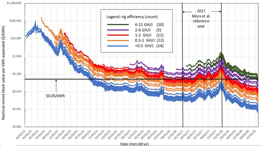
3 Next, for each of the 62 rigs in the authors’ selection pool, we calculated the electricity use that would
 4 be necessary if that rig were assigned to solve the blocks in each day k, following the mathematical
 5 approach in Eq. 1. Finally, we divided the nominal mined block value (Vk) by the electricity use that
 6 would have been required for a given rig to solve those blocks (kWh), and did so for all days in our
 7 analysis period.

 8 Supplementary Fig. 5 plots our computed nominal mined block value per kWh expended ($/kWh) for all
 9 62 rigs. This metric expresses the maximum mining value that could be extracted per kWh expended
10 during mining; when operating costs per kWh expended ($/kWh) exceed this value, mining cannot be
11 profitable. Operating costs include the costs of electricity, equipment depreciation, labor, and other
12 costs incurred during mining. While empirical data on operating costs are scarce, several published
13 estimates suggest that $0.05/kWh is a reasonable current minimum value, with electricity typically
14 comprising the largest share of operating costs.7,15

15 In Supplementary Fig. 5, we color code rigs of different efficiency classes, indicate the numbers of rigs
16 that fall into each class in the authors’ selection pool, and start each rig’s data series on its estimated
17 release date. We also indicate the typical $0.05/kWh threshold on the plot; rigs whose data series fall
18 below this threshold in a given time period would not be considered profitable, because nominal mined
19 block value earned per kWh expended would not exceed operating costs.

20 It can be seen that many of the older, less energy-efficient rigs that were included in the authors’
21 selection pool—while profitable when first introduced several years ago—by 2017 would be profitable
22 only at implausibly low operating cost levels. For example, in 2017, many of the lowest efficiency rigs
23 included by the authors (i.e., the blue-shaded rigs with efficiencies less than 0.3 GH/J) could have only
24 been profitable with operating costs less than $0.01/kWh, which is much lower than even the cheapest
25 documented rates for mining electricity costs alone.15,16,17

26 In other words, many of the rigs included in the authors’ selection pool were not “economically
27 profitable by modern standards” in the authors’ own reference year (2017), and should, therefore, have
28 been excluded from their analysis. In Supplementary Fig. 6, we plot the effects of excluding old, energy-
29 efficient rigs from our replicated analysis at different assumed levels of operating cost. For each
30 monthly period in 2017, we reran our original replication but excluded any rigs from the selection pool
31 that would not have been profitable at various operating cost levels. We summed these monthly results
32 to arrive at total direct Bitcoin electricity use estimates in 2017.

33 It is clear from Supplementary Fig. 6 that inclusion of old, energy-efficient rigs in the authors’ analysis
34 resulted in an inflated 2017 direct electricity use estimate. Even if the authors had excluded rigs that
35 were not profitable at implausibly low operating costs of $0.01/kWh, their 2017 electricity use estimate
36 would have dropped nearly in half, from 114 TWh to 62 TWh, while their 2017 CO2 emissions estimate
37 would have dropped from 69 Mt CO2e to 38 Mt CO2e. At the generally-accepted minimum operating
38 cost level of $0.05/kWh, the authors’ 2017 electricity use and CO2 emissions estimates would have
39 dropped much further, to 28 TWh and 17 MtCO2e, respectively. These latter values are more consistent
40 with other published estimates of Bitcoin’s 2017 direct electricity use and related carbon emissions,
41 which include only the newer, faster, and more energy-efficient rigs that were likely to be profitable in
42 2017.5-7 Indeed, looking at Supplementary Fig. 6 from left to right, one can clearly see how, as rigs get
43 older, they are invariably pushed out of profitability as newer, more efficient rigs emerge.

 11

Supplementary Figure 5. Nominal mined block value per kWh expended for the 62 mining rigs included in the authors’ selection pool

 12

1
 2 Supplementary Figure 6. Mora et al. model estimates of 2017 Bitcoin electricity use and CO2 emissions
 3 when unprofitable rigs were excluded from their selection pool, at different operating cost
 4 assumption levels.

 5 Furthermore, the authors applied 2014 carbon intensities (g CO2/kWh) to their 2017 electricity use
 6 estimates, ignoring non-negligible grid decarbonization improvements in their assumed mining locations
 7 during the intervening years (Supplementary Fig 7). This was done even though sufficient data existed at
 8 the time of their study for reasonable estimates of 2017 carbon intensities.18,19,20 Supplementary Fig. 7
 9 plots the location-weighted average grid CO2 emissions intensity from 2000-2016 (historical), with
10 forward-projections from 2017 to 2060 from the IEA’s central outlook (based on current and announced
11 national policies in assumed mining locations). From this figure, it’s clear that, by using 2014 carbon
12 intensities, the authors arrived at a higher 2017 CO2 emissions value than if they had used available data
13 for 2017 carbon intensities.

14 To assess the effects of the authors’ use of outdated rig efficiencies and grid carbon intensities, we
15 applied our replicated Mora et al. model to estimate 2017 Bitcoin CO2 emissions using more reasonable
16 assumptions. Based on the assumption that $0.05/kWh represents the global average minimum Bitcoin
17 mining operating cost—and excluding rigs that did not yield nominal mining revenues per kWh
18 expended exceeding $0.05/kWh in 2017—the authors’ model yielded an estimate of 28 TWh
19 (Supplementary Fig. 6). We then multiplied this value by a location-weighted carbon intensity that was
20 9% lower than the authors’ 2014 value, to capture the technological progress that occurred between
21 2014 and 2017 (Supplementary Fig. 7). We arrived at a 2017 Bitcoin CO2 emissions estimate of 15.7
22 MtCO2e, which is far lower than the authors’ original estimate of 69 MtCO2e.

 13

23 Therefore, we determined that, had the authors not erroneously included outdated rig efficiencies and
24 grid carbon intensities, their own model would have estimated substantially lower 2017 energy use and
25 CO2 emissions values, invalidating their original results.

26
27 Supplementary Figure 7. Location-weighted average electric power direct carbon intensity using
28 historical (2000-2016) and projected (2017-2060) data available at the time of the authors’ study. Also
29 shown is the level of direct carbon intensity locked into the authors’ estimates by assuming static
30 2014 carbon intensity values. Location-weighted average assumes the following percentages of 2017
31 Bitcoin electricity use by region, according to the locations assigned by the authors to each solved
32 block: China (62.2%), U.S./China average (9.3%), U.S. (3.9%), global average (17%), Georgia, Finland,
33 and Iceland (5.3%), U.S./E.U. average (0.1%), India (2.3%), and Sweden (0.1%).

34

35 VII. Holding both mining rig efficiency and grid carbon intensity constant in all future years

36 As evident in Eq. 2, the authors applied their 2017 per-transaction CO2 emissions values in all future
37 years, multiplying them by annual transactions to obtain future CO2 emissions trajectories for each
38 scenario. This was done by sampling solved blocks from their 2017 analysis until the required
39 transactions in each future year were fulfilled. In other words, they did not vary the mining rig pool
40 options in future years; for example, the pool of rigs they used to solve blocks in 2050 was the same
41 pool of rigs they used to solve blocks in 2017. Moreover, the authors state explicitly that they did not
42 consider any changes over time to the power grids in each assumed mining location. These decisions
43 effectively held both mining rig efficiencies and grid carbon intensities constant for the next 100 years.

 14

44 This dubious choice ignores the dynamic natures of mining rig and power grid technologies and violates
45 the widely-followed practice of accounting for technological change in forward-looking energy
46 technology scenarios.

47 Estimating the future energy efficiency of mining is certainly difficult, but the authors never explain why
48 they simply ignored this important scenario consideration, nor do they justify how assuming static
49 mining efficiencies for 100 years—when, historically, mining rigs have evolved monthly with respect to
50 their hashrates and energy efficiencies— can lead to any useful insights. And, in acknowledging their
51 static grid intensities assumption, they point to at least one available reference containing credible grid
52 intensity outlooks,20 but failed to utilize these data. The fallacy in keeping grid carbon intensities
53 constant at 2014 levels can clearly be seen in Supplementary Fig. 7, which shows a widening gulf over
54 time between the authors’ static assumption (in red) and that of the prevailing outlook (the IEA’s ETP
55 2017 Reference Technology Scenario, in green) for the authors’ assumed mining locations.

56 We consider the authors’ decisions to hold both mining rig efficiencies and grid carbon intensities
57 constant to be fatal flaws of their analysis, and conspicuously out of step with established best practices
58 for IT energy analysis and long-term energy scenario modeling.21 And, because the authors significantly
59 overestimated 2017 Bitcoin energy use and CO2 emissions by using outdated rig and carbon intensity
60 data, it follows that their decision to lock in these 2017 values in all future years led to inflated CO2
61 emissions projections as well.

62 Therefore, we assessed how the authors’ own model would have yielded different results had they: (a)
63 at least excluded unprofitable rigs from their 2017 pool; and (b) used available data sources to account
64 for projected changes in grid carbon intensities in their assumed mining locations. We applied our
65 replicated model to first generate scenarios assuming 2017 CO2 emissions of 15.7 MtCO2e (based on a
66 global average minimum operating cost of $0.05/kWh, as discussed in Section VI), as shown in
67 Supplementary Fig. 9b. To these results, we then applied changes in the location-weighted grid carbon
68 intensity from 2017 to 2060, using available data from the IEA’s central outlook based on current and
69 announced national policies in each mining location (Supplementary Fig. 9c).

70 The results show that, had the authors applied more reasonable values in their analysis—even
71 maintaining the flawed assumption of holding 2017 mining rig efficiencies constant, but at more
72 economically plausible levels—their own model would have delivered much different projections
73 compared to their original results.

74 VIII. Improper execution of the 40-product comparison analysis

75 Lastly, our replication of the authors’ 40 technology comparison (see Section III) revealed errors that
76 biased their results in favor of steep initial growth trajectories. While the scientific community may be
77 justified in questioning the authors’ comparison of Bitcoin to a seemingly arbitrary mix of technologies
78 that vary widely in their social utility, here we focus only on errors committed by the authors executing
79 their own stated methods.

80 In constructing their scenarios, the authors state that “the first year of usage for each technology was
81 set to one, to allow comparison of trends among technologies,” which is the approach we followed in
82 our replicated analysis (Supplementary Fig. 2). For each technology, the authors equated “first year of
83 usage” with “first year since introduction,” as evident in their Fig 1b. However, in our replicated

 15

84 analysis, we discovered that, for many technologies, the authors erroneously assumed that the first
 85 nonzero value available in the source data represented the first year of actual technology use.

 86 For example, the authors designate the first year of usage for the automobile as 1915, at which point US
 87 household adoption was already 10%. However, the modern automobile was invented in the late
 88 1890s, with mass production starting in the United States around 1901.22 Similarly, the authors
 89 designate the first year of usage for electric power as 1908, at which point US household adoption had
 90 also climbed to 10%. Yet Thomas Edison began offering electric power to customers in Manhattan over
 91 two decades earlier, in 1882.23 We found similar discrepancies for other technologies in the authors’
 92 comparison pool, which are documented in Supplementary Table 2.

 93 By erroneously assuming that the first available adoption number in the source data represented the
 94 first year of technology availability, the authors omitted the initial low-adoption years of US market
 95 availability for numerous technologies. Mathematically, these omissions biased the authors’ scenarios
 96 toward inaccurately steep near-term adoption trajectories in all three cases.

 97 To illustrate this point, we repeated the authors’ approach using more realistic values for the first year
 98 of technology usage obtained from the literature,55-83 as summarized in Supplementary Table 2.
 99 Adoption rates in the initial years were estimated using linear interpolation. We also removed three
100 duplicative entries from the authors’ 40 product comparison pool (computers, refrigerators, and
101 washing machines) and NOx controls (the rapid adoption of which was driven by regulatory mandates,
102 not market demand), as noted in the table.

103 Our adjusted median, lower25, and upper75 curves are shown in Supplementary Fig. 8, which were
104 based on the best-fitting regression models for each data series. It can be seen that more realistic
105 estimates for the first year of technology use, and a more coherent comparison pool drawn from the
106 same data sources, would result in a fast scenario (i.e., upper75) with less aggressive logarithmic growth
107 and median and slow (i.e., lower25) scenario curves that are demonstrably less steep in the near term
108 than those constructed by the authors.

109 To assess how the authors’ errors in their own scenario derivations affected their results, we reran our
110 replicated emissions projection once again using the adjusted Bitcoin adoption scenarios in
111 Supplementary Fig. 8. The results are plotted in Supplementary Fig. 9d. By correcting the authors’ own
112 scenario analysis as the last step in the cascade of corrections we discuss, we show that their model
113 would have now projected CO2 emissions trajectories that would not have crossed the 2oC threshold
114 until between 2075 to 2110.

115

 16

116
117 Supplementary Figure 8. The authors’ Bitcoin adoption scenarios based on more realistic first year of
118 usage estimates within the technology comparison pool.

119

120

 17

121
122

123 Supplementary Figure 9: Comparison of Bitcoin CO2 emissions projected by the Mora et al. model: (a)
124 our replicated analysis showing close agreement with the authors’ results; and the model’s
125 projections after first (b) removing unprofitable rigs in the base year, then (c) accounting for evolution
126 of the electric power grid in mining locations, and finally (d) correcting errors in their stated adoption
127 scenario approach.

 18

Supplementary Table 2. Authors’ selected versus more reasonable first year of usage values for
comparative technologies

 Authors’ assigned Actual first year Initial years of
 first year of usage of usage (YSI = availability omitted
 Technology (YSI = 1) 1) by the authors
 Automatic transmission 1951 1939 12
 Automobile 1915 1901 14
 Cable TV 1968 1948 20
 Cellular phone 1994 1984 10
 Central heating 1920 1892 28
 Colour TV 1966 1954 12
 Computer 1992 Duplicate -
 Dishwasher 1922 1922 -
 Disk brakes 1966 1963 3
 Dryer 1950 1938 12
 Ebook reader 2009 1998 11
 Electric Range 1933 1908 25
 Electric power 1908 1882 26
 Electronic ignition 1977 1963 14
 Flush toilet 1860 1860 -
 Freezer 1950 1947 3
 Home air conditioning 1957 1931 26
 Household refrigerator 1931 Duplicate -
 Internet 1993 1991 2
 Landline 1903 1885 18
 Microcomputer 1984 1984 -
 Microwave 1975 1955 20
 Nox pollution controls 1990 1990 -
 Podcasting 2006 2003 3
 Power steering 1951 1951 -
 RTGS adoption 1970 1970 -
 Radial tires 1972 1967 5
 Radio 1925 1921 4
 Refrigerator 1925 1918 7
 Running water 1890 1833 57
 Shipping container port inf. 1964 1955 9
 Smartphone usage 2011 2000 11
 Social media usage 2005 1997 8
 Stove 1900 1900 -
 Tablet 2010 1992 18
 Vacuum 1922 1908 14
 Washer 1920 1907 13
 Washing machine 1930 Duplicate -
 Water Heater 1933 1904 29
 Debit card 1995 1984 11

 19

References

1
 Our World in Data. Technology adoption by households in the United States. (2019).
https://ourworldindata.org/grapher/technology-adoption-by-households-in-the-united-
states?time=1903..2016

2
 Consumer Credit and Payment Statistics (Federal Reserve Bank of Philadelphia);
https://www.philadelphiafed.org/consumer-finance-institute/statistics

3
 Encyclopaedia Brittanica, The Credit Card. https://www.britannica.com/topic/credit-card

4
 U.S. Federal Reserve. Credit Cards: Use and Consumer Attitudes, 1970–2000. (2000).
https://www.federalreserve.gov/Pubs/Bulletin/2000/0900lead.pdf
5
 Vranken, H. Sustainability of bitcoin and blockchains. Current Opinion in Environmental Sustainability
28, 1-9, doi:https://doi.org/10.1016/j.cosust.2017.04.011 (2017).

6
 Krause, M. J. & Tolaymat, T. Quantification of energy and carbon costs for mining cryptocurrencies.
Nature Sustainability 1, 711-718, doi:10.1038/s41893-018-0152-7 (2018).

7
 Bevand, M. Op Ed: Bitcoin Miners Consume A Reasonable Amount of Energy — And It's All Worth It,
 (2017).

8
 Bitcoinity. Data.bitcoinity.org. (2019).

9
 Bitcoinity. Number of transactions - Bitcoinity.org. (2019).
http://data.bitcoinity.org/bitcoin/tx_count/5y?t=l

10
 Koomey, Jonathan G, Chris Calwell, John A Laitner, Jane Thornton, Richard E Brown, Joseph H Eto,
Carrie A Webber, and Cathy Cullicott. "Sorry, wrong number: The use and misuse of numerical facts in
analysis and media reporting of energy issues." Ed. Socolow, Robert H, Dennis Anderson, and John
Harte. Annual Review of Energy and the Environment 2002 27 (2002) 119-158. LBNL-50499.

11
 Koomey, Jonathan, Huimin Chong, Woonsien Loh, Bruce Nordman, and Michele Blazek. 2004.
"Network electricity use associated with wireless personal digital assistants." The ASCE Journal of
Infrastructure Systems (also LBNL-54105). vol. 10, no. 3. September. pp. 131-137.
[http://ascelibrary.org/doi/abs/10.1061/(ASCE)1076-0342(2004)10%3A3(130)]

12
 Koomey, J. Turning Numbers into Knowledge: Mastering the Art of Problem Solving. (Analytics Press,
2017).

13
 Camilo Mora, Randi L. Rollins, Katie Taladay, Michael B. Kantar, Mason K. Chock, Mio Shimada & Erik
C. Franklin. Bitcoin emissions alone could push global warming above 2°C. Nature Climate
Changevolume 8, pages931–933 (2018)

 20