An open access dataset for developing automated detectors of Antarctic baleen whale sounds and performance evaluation of two commonly used ...
←
→
Page content transcription
If your browser does not render page correctly, please read the page content below

www.nature.com/scientificreports
OPEN An open access dataset
for developing automated
detectors of Antarctic baleen
whale sounds and performance
evaluation of two commonly used
detectors
Brian S. Miller1*, The IWC-SORP/SOOS Acoustic Trends Working Group*, Naysa Balcazar2,
Sharon Nieukirk3, Emmanuelle C. Leroy4, Meghan Aulich5, Fannie W. Shabangu6,7,
Robert P. Dziak3, Won Sang Lee8 & Jong Kuk Hong8
Since 2001, hundreds of thousands of hours of underwater acoustic recordings have been made
throughout the Southern Ocean south of 60° S. Detailed analysis of the occurrence of marine mammal
sounds in these circumpolar recordings could provide novel insights into their ecology, but manual
inspection of the entirety of all recordings would be prohibitively time consuming and expensive.
Automated signal processing methods have now developed to the point that they can be applied
to these data in a cost-effective manner. However training and evaluating the efficacy of these
automated signal processing methods still requires a representative annotated library of sounds to
identify the true presence and absence of different sound types. This work presents such a library of
annotated recordings for the purpose of training and evaluating automated detectors of Antarctic blue
and fin whale calls. Creation of the library has focused on the annotation of a representative sample of
recordings to ensure that automated algorithms can be developed and tested across a broad range of
instruments, locations, environmental conditions, and years. To demonstrate the utility of the library,
we characterise the performance of two automated detection algorithms that have been commonly
used to detect stereotyped calls of blue and fin whales. The availability of this library will facilitate
development of improved detectors for the acoustic presence of Southern Ocean blue and fin whales.
It can also be expanded upon to facilitate standardization of subsequent analysis of spatiotemporal
trends in call-density of these circumpolar species.
Underwater passive acoustic monitoring (PAM) for marine mammals is a fast-growing field due to increased
availability of, and flexibility in deploying, underwater recording d
evices1–3. PAM has especially high potential
to provide information about marine mammals in remote or difficult to access areas, such as Antarctic waters.
Since 2001, hundreds of thousands of hours of long-term acoustic recordings that span many years have been
collected throughout the Southern Ocean. Many of these recordings were made for the purposes of learning about
two endangered species that are especially detectable by PAM: Antarctic blue whales (Balaenoptera musculus
intermedia) and fin whales (B. physalus)4.
1
Australian Antarctic Division, 203 Channel Highway, Kingston Tasmania, Australia. 2Unaffiiliated, Brisbane,
QLD, Australia. 3Pacific Marine Environmental Laboratory, NOAA, Newport, OR, USA. 4Unaffiliated, Bretagne,
France. 5Centre for Marine Science and Technology, Curtin University, Bentley, WA, Australia. 6Department of
Environment, Forestry and Fisheries, Fisheries Management Branch, Cape Town, South Africa. 7Mammal Research
Institute Whale Unit, University of Pretoria, Hatfield, Private Bag X20, Pretoria 0028, South Africa. 8Korea Polar
Research Institute, Incheon 21990, South Korea. *A list of authors and their affiliations appears at the end of the
paper. *email: brian.miller@aad.gov.au
Scientific Reports | (2021) 11:806 | https://doi.org/10.1038/s41598-020-78995-8 1
Vol.:(0123456789)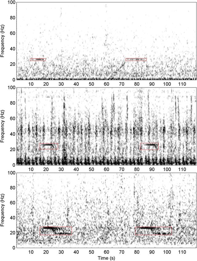
www.nature.com/scientificreports/
Monitoring blue and fin whales in the Southern Ocean. Historically, blue whales were heavily
exploited throughout the Southern Ocean. Approximately 360,000 blue whales were caught across the South-
ern Hemisphere in the mid-twentieth century, depleting the population to less than 1% of their pre-whaling
population5. The most recent abundance estimate of Antarctic blue whales suggest that the population contained
between 1140 and 4440 individuals and may be slowly increasing at a rate between 1.6 and 14.8% per year (95%
CI; mean of 8.2%), however this estimate was for the Antarctic summer of 1997/98, and thus is now dated by
more than 20 years6. Over 725,000 fin whales were caught during the twentieth century7, yet circumpolar abun-
dance of Southern Ocean fin whales has never been estimated since extant data sources are not sufficient to do
so with fidelity8.
Given the endangered status of both blue and fin whales globally, the critically endangered status of Antarc-
tic blue whales9, and the fact that both are long-lived species that are believed to reproduce every 2–3 years10,
long-term monitoring is imperative to examine population trends and the effectiveness of current conservation
measures (e.g. the moratorium on commercial whaling; https://iwc.int/commercial). PAM from fixed sensors
is an ideal method for obtaining cost-effective broad spatial and long-term temporal coverage of blue and fin
whale occurrences throughout a vast Southern Ocean region that is challenging to access. Blue and fin whales
each produce distinct calls that can be repeated as songs, or produced as individual notes, which are unique to
their respective species. In the case of Antarctic blue whales some sounds are unique to their population11–13.
The repeated, loud, low-frequency, and long-travelling calls from these endangered species provide an extremely
efficient means of identifying the presence of whales in the remote Antarctic waters of the Southern Ocean.
The Antarctic Blue and Fin Whale Acoustic Trends Project started in 2009 as one of the original projects of the
International Whaling Commission’s Southern Ocean Research Partnership (IWC-SORP; https://iwc.int/sorp),
and in 2017 expanded further to become a capability working group of the Southern Ocean Observing System
(SOOS; www.soos.aq). The overarching goal of this project is to use acoustics to examine trends in Antarctic blue
and fin whale population growth, abundance, distribution, seasonal movements and behaviour.
Through IWC-SORP, the Acoustic Trends Project working group has built upon the pioneering work done
in the first decade of the twenty-first century, and has fostered an increasing number of passive acoustic studies
focusing on the calls of Antarctic blue whales and to a lesser extent fin whales across broad time and spatial
scales, as well as acoustic data processing and analysis methodology. The data from these studies have been
collected both from ships during Antarctic voyages and from long-term moored recording d evices4,14–31. The
project working group presently (as of March 2020) has access to more than 300,000 h of passive acoustic data
that have been collected throughout the Southern Ocean over the past 20 years.
Automated detection of whale sounds. The volume of existing and incoming acoustic data far exceeds
the capacity of human expert analysts to manually inspect it, and as a result automated algorithms have been
relied upon to determine the presence of sounds from marine mammals in the recordings. Ecological results
from long-term analyses have been reported in the form of presence (e.g. months, days, or hours of recordings
with call presence), or as estimates of call numbers per time-period (e.g. see studies listed in Table 1). How-
ever, the results are not easily comparable because different studies had different data collection protocols and
employed different analytical techniques, neither of which have been standardised. Furthermore, robust meas-
ures of bias and variability, which can be dataset-specific, are not always reported alongside results (Table 1).
A variety of automatic detection algorithms have been used to detect the calls of blue whales and fin whales.
Algorithms to detect stereotyped calls of these species include matched fi lters32–34, energy d
etectors35, subspace
projection detectors (blue whales only26,36). However, the most widely used algorithm has been spectrogram
correlation37, and this has been implemented in a variety of software p ackages38–40 and has been used widely on a
variety of different datasets16–20,30,41–44. Spectrogram correlation is similar to matched filtering except that it acts on
the spectrogram, rather than purely in the time or frequency domains; instead of cross-correlating a time series
or spectrum, it correlates an image template or kernel pixel-by-pixel with the spectrographic data of interest.
Factors that affect the detector performance. Three main factors can impact the performance of
an automated detection algorithm: acoustic properties of the recording site, variability in signals that are being
detected, and variability in the characteristics of the recording system. The acoustic recordings from the South-
ern Ocean span a wide geographic and temporal range and encompass a variety of environments, thus char-
acteristics of the recording site (e.g. propagation loss and noise levels) are expected to be both site- and time-
specific43,46.
In addition to site-specific features, the properties of blue and fin whale sounds can change over time and
space. Sounds from most blue whale populations have changed slowly and in a predictable manner since they
were first described in the 1 970s14,47–49. On top of the well documented decreases in tonal frequency of sounds
from year-to-year, there are predictable intra-annual changes that have also been o bserved14,48,50. There is some
evidence that the properties of fin whale sounds vary geographically in the A ntarctic15,18, and have been found
to vary temporally in other o ceans33,51,52. While these changes may seem small and/or occur over long time
periods, they must nevertheless be accounted for when using automated detection algorithms to detect trends
in long-term and widely dispersed d atasets53.
Lastly, the acoustic recordings around the Antarctic have been made with a variety of instruments. These
include: Scripps Acoustic Recording Packages (ARP); Multi-Electronique Autonomous Underwater Recorder for
Acoustic Listening (AURAL); Australian Antarctic Division Moored Acoustic Recorders (AAD-MAR), Develogic
Sono.Vaults; and Pacific Marine Environmental Laboratory—Autonomous Underwater Hydrophones (PMEL-
AUH). Different instruments may have different capabilities, including depth rating, system frequency response,
and duty cycle requirements, and these further affect the performance of an automated detector54. For example,
Scientific Reports | (2021) 11:806 | https://doi.org/10.1038/s41598-020-78995-8 2
Vol:.(1234567890)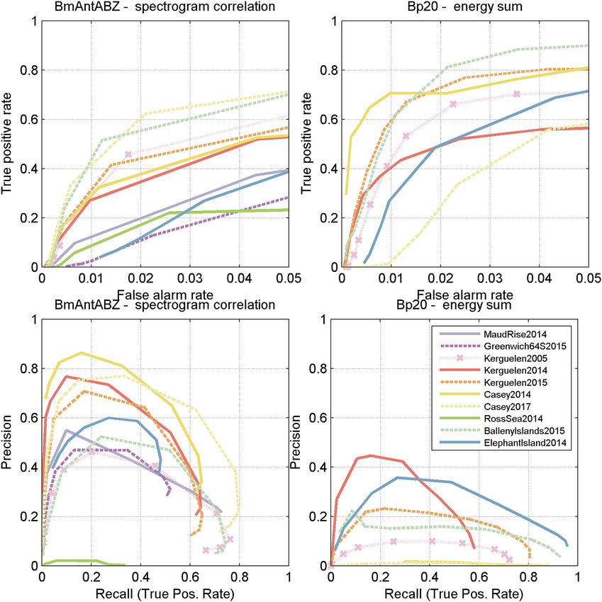
www.nature.com/scientificreports/
Detection method Characterisation/
Study (software used) Noise pre-processing True positive rate False positive rate False positive removal validation summary
Threshold was iteratively
Spectrogram correlation adjusted until false positive
17
Širović et al. 2004 (Ishmael) Not reported Not reported < 1% No rate was < 1%. Calls on days
Energy sum (Ishmael) with fewer than 50 detec-
tions were inspected
Visual inspection of all
Spectrogram correlation
Širović et al. 200918 Not reported Not reported Not reported All detections to remove false
(Ishmael)
positives
Months with fewer than
50 detections: visual
inspection of detections to
Spectrogram correlation
Samaran et al. 201330 Not reported Not reported 6%a Some remove all false positives.
(XBAT)
Otherwise 10% of ran-
domly selected detections
inspected
Visual inspection of all
Tripovich et al. 201520 Energy detection (Ishmael) Not reported Not reported 14.6% All detections to remove false
positives
False detection rates and
thresholds determined via
Spectrogram correlation detection function quan-
Thomisch et al. 201619 Not reported Not reported Nominally < 1% No
(custom developed) tiles from 100
randomly selected
detectionsb
Detections deemed false if
Subspace projection the frequency at maximum
Leroy et al. 201626 Noise-adaptive threshold Not reportedc Nominally < 3% Some
detection36 amplitude was different
than that of unit-A
Comparison against expert
human observer who anno-
tated 1 randomly selected
Balcazar et al. 201745 Energy sum (Ishmael) Not reported 93.3–97.3% 14.6–98.9% All day each month for each
site. Visual inspection of all
detections to remove false
positives
20% subset of days with no
automated detections visu-
Spectrogram correlation ally inspected to determine
Buchan et al. 201742 Not reported 99.998%d Not reported All
(Ishmael) false negative rate. Visual
inspection of all detections
to remove false positives
Visual inspection of entire
Spectrogram correlation dataset (1518 h) to assess
Shabangu et al. 201716 Not reported 42–83% Not reported All
(XBAT) remove false positives and
include missed detections
Table 1. Previous analyses of long-term datasets that have used automated algorithms to detect calls and
report spatial distribution and/or temporal occupancy of Antarctic blue whales. a False positive rate reported
only for months when there were more than 500 calls detected. b False positive detections were from a different
detector operating in an adjacent frequency band with a similar, frequency-adjusted, spectrogram correlation
kernel. c True positive rates for this detector for high, medium, and low signal to noise ratio (SNR) calls and a
variety interfering noises reported by Socheleau et al. 2015, but the prevalence of these conditions within the
full dataset is not indicated. d False negative rate reported as a percentage of total uncorrected detections for a
20% subset of days without automated detections.
the duty cycle of an instrument, for example, is known to affect the accuracy of predicting the presence of Ant-
arctic blue whales in addition to the call rate55. Additionally, the depth of the recorder is expected to change the
detection range and noise levels observed at a recorder4.
Here we create and document an open access set of recordings collected around the Antarctic and manual
annotations of blue and fin whale call occurrences in a subset of those recordings. This dataset takes the form of
an “annotated library” of Antarctic underwater sound recordings. We demonstrate how the library can be used
to evaluate the performance of automated detectors over the variety of recording scenarios contained within
the library. We also suggest methods to help standardise the reporting of results with a view towards facilitating
long-term comparisons of PAM studies of baleen whales around Antarctica.
Methods
Towards a representative circumpolar dataset. Our annotated library contains data from four geo-
graphic regions: the Atlantic, Pacific, and Indian sectors of the Southern Ocean and the Western Antarctic Pen-
insula (WAP; Fig. 1). In each region, we identified sites that had at least a full year of data from 2014 or 2015,
and ideally had two consecutive years. When two consecutive years were not available, another year from the
same site was included or two different sites were selected. The Indian sector site also included data from 2005
to increase the temporal span of the library, as well as a second location with data from 2014 and 2017. The data
Scientific Reports | (2021) 11:806 | https://doi.org/10.1038/s41598-020-78995-8 3
Vol.:(0123456789)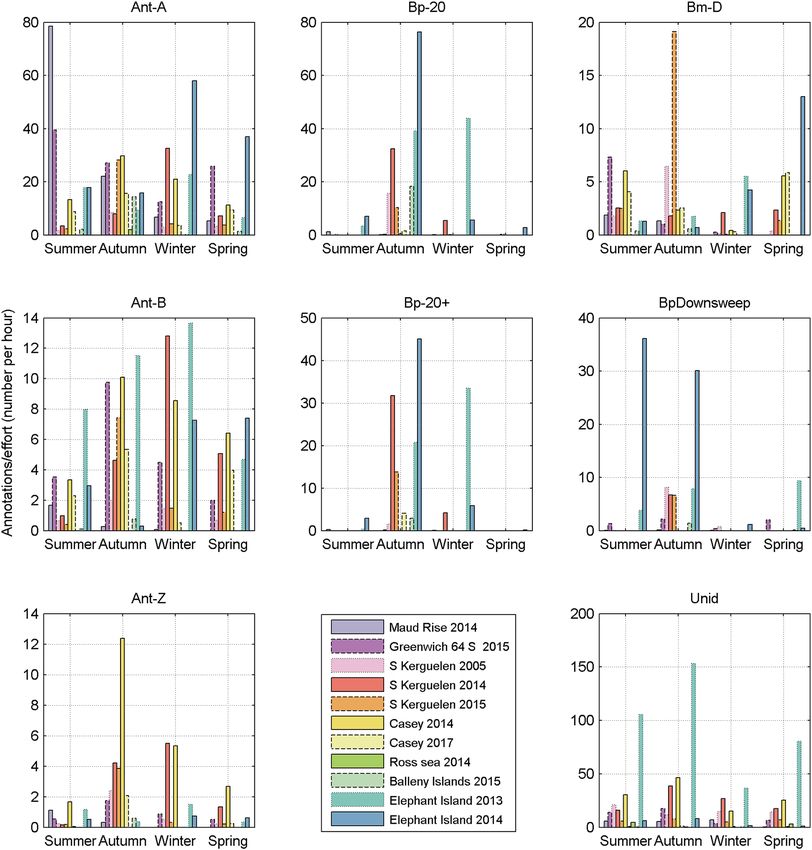
www.nature.com/scientificreports/
Figure 1. Map of Antarctic underwater recording sites illustrating sites used in this study (red circles) and
known locations of long-term recordings from 2001 to 2017 (open circles). Map created using M_Map version
1.4k56 and ETOPO 1 bathymetry (https://www.eoas.ubc.ca/~rich/map.html). Light, medium, and dark blue lines
show 1000, 2000, and 3000 m depth contours respectively.
Unique calendar Unique calendar
Dataset name (site- hours with days with Audio duration
year) Latitude Longitude Analyst Instrument Start Stop annotations annotations annotated (h)
Maud Rise 2014 65° 0.00′ S 2° 30.00′ E BSM AURAL 2014-01-12 2014-09-17 201 201 83.3
Greenwich 64S 2015 64° 00.32′ S 0° 00.22′ E NB Sono.Vault 2015-01-02 2015-12-31 190 190 31.7
S Kerguelen Plateau
62° 35.44′ S 81° 15.64′E NB ARP 2005-01-31 2006-01-31 200 200 200
2005
S Kerguelen Plateau
62° 22.81′ S 81° 47.81′ E NB AAD-MAR 2014-02-22 2015-02-20 200 200 200
2014
S Kerguelen Plateau
“ “ NB AAD-MAR 2015-02-10 2016-01-27 200 200 200
2015
Casey 2014 63° 47.73′ S 111° 47.23′ E NB AAD-MAR 2013-12-25 2014-12-12 194 194 194
Casey 2017 “ “ MA AAD-MAR 2016-12-15 2017-11-07 185 185 185
Ross Sea 2014 75° 01.19′ S 164° 35.51′ E SN PMEL-AUH 2014-02-08 2014-12-14 176 176 176
Balleny Islands 2015 65° 21.34′ S 167° 54.69′ E SN PMEL-AUH 2015-01-15 2016-01-10 205 205 204
Elephant Island 2013 61° 00.88′ S 55° 58.53′ W NB AURAL 2013-01-12 2013-12-02 2247a 93a 187a
Elephant Island 2014 “ “ ECL AURAL 2014-01-01 2014-12-31 2592 108 216
Table 2. Description of annotated datasets including the site-year, location, initials of the analyst who made
the annotations, type of instrument, start and stop date of the annotations, and number of hours (independent
dates and times) annotated, as well as the total duration of the recordings annotated. a Not evenly distributed
throughout the year.
in this library were recorded using a variety of instruments: ARP, AURAL, AAD-MAR, Sono.Vault; and PMEL-
AUH (Table 2).
Subsampling from each dataset. Moorings in the Antarctic are typically recovered and serviced at the
most once a year due to their remote locations, potentially long periods of ice cover, and reduced/negligible
access during Antarctic winter. Thus we define a site-year as a recording from a single instrument and site that
is approximately a year in duration. A subset of approximately 200 h of data was selected from each site-year
for annotation. This number of hours was chosen a priori and was constrained by budgetary limits, but it was
believed to be a reasonable trade-off among analyst time, maintaining adequate sample sizes within each site-
year, and annotating a sufficient number of different site-years.
For each site-year a systematic random subsampling scheme was used to generate a representative set of
acoustic recordings from the larger dataset. The systematic random subsampling scheme consisted of:
Scientific Reports | (2021) 11:806 | https://doi.org/10.1038/s41598-020-78995-8 4
Vol:.(1234567890)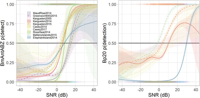
www.nature.com/scientificreports/

                                 Figure 2.  Number of hours annotated for each month for each site-year.

                                 1. splitting the dataset into “chunks” of time. The optimal length of a time chunk will be species and study
                                    specific. For the annotated library time was split into mostly hour-long chunks with some exceptions.
                                 2. calculating the spacing between chunks, ts to ensure that the desired sample size of time chunks is created and
                                    that there was broad representation of hours in the day across all chunks. For the annotated library, spacing
                                    was calculated such that there were at least 150, and usually nearer to 200, annotated periods between the
                                    first and last available chunks.
                                 3. Picking a random number between 1 and ts, the spacing, to determine the starting chunk (this was the ran-
                                    dom element of the subsampling scheme).

                                     The aim of the subsampling scheme was to capture a representative sample of the signals recorded for a given
                                 site-year, i.e., to select periods of time with calls that spanned a range of signal-to-noise ratios (SNR) and periods
                                 of time without calls, as well as other sounds that might contribute to false positives (though rare events may have
                                 been missed). Having a temporally representative subsample of sounds was deemed necessary to understand
                                 how a detector would perform when used across the entire dataset.
                                     For each site, 10–18 h of data were annotated per month with the exceptions of the Ross Sea in 2014 which
                                 had no data for January, and Maud Rise 2014 which recorded only from Jan-Sep (Fig. 2). Over the whole year the
                                 subsampling scheme ensured a relatively even distribution of hours across a 24 h cycle, with each site containing
                                 between 5 and 10 h inspected for any given hour in the cycle.
                                     However, four sites had been annotated previously, and thus used slightly different subsampling schemes.
                                 Additionally, three of these sites had recording duty cycles shorter than an hour. Elephant Island 2013 and 2014
                                 had a duty cycle of 5 min/h. Maud Rise 2014 had a duty cycle of 25 min/hour. For Elephant Island 2014 9 days
                                 per month were selected (randomly, but with roughly even spacing between them), and all 5 min segments were
                                 analysed for selected days (total duration of all audio segments 216 h). For Maud Rise 2014 200 independent
                                 evenly spaced hours were selected and each 25 min segment was analysed (total duration of all audio segments
                                 83.3 h). For Elephant Island 2013 all 5 min segments for every day were analysed from 12 Jan 2013 to 8 Apr
                                 2013. For the remaining months (May–Dec 2013) all segments from one day each month were analysed. Lastly,
                                 Greenwich 64 S 2014 had 10 min long sub-samples that were annotated. These were spread over 190 unique
                                 hours throughout the year (31.6 h audio duration).

                                 Manual annotations. For manual detection and annotation of calls, recordings were visualised in Raven
                                 Pro 1.557. Spectrogram details included a 120 s timespan, frequency limits between 0 and 125 Hz, Fast Fourier
                                 Transform (FFT) of approximately 1 s in duration; frequency resolution of approximately 1.4 Hz, and 85% time
                                 overlap between successive FFTs. Lower and upper limits of the spectrogram power (spectrogram floor and ceil-
                                 ing) were adjusted for each 1-h segment. The lower limit of spectrogram power was adjusted by the analyst until
                                 approximately 25% of the spectrogram was at or below the floor value (i.e. a visual estimate of 25th percentile
                                 spectral noise level). The ceiling of the spectrogram was then adjusted so that the difference between ceiling
                                 and floor was between 30 and 50 dB relative to full-scale. The ceiling of the spectrogram could then be adjusted
                                 further to provide additional contrast in the event of long loud broadband sounds such as ice or prolonged
                                 occurrence of baleen whale choruses.
                                     Within each subsample the analyst marked the time–frequency bounds of all occurrences of blue and fin
                                 whale sounds. Each analyst had extensive expertise in the identification of blue and fin whale sounds, particu-
                                 larly those from the Southern Hemisphere including the Antarctic. The analyst assigned one of eight different
                                 classifications to annotations: Bm-Ant-A, Bm-Ant-B, Bm-Ant-Z, Bm-D, Bp-20, Bp-20Plus, Bp-Downsweep, and

Scientific Reports |   (2021) 11:806 |                https://doi.org/10.1038/s41598-020-78995-8                                                     5

                                                                                                                                                Vol.:(0123456789)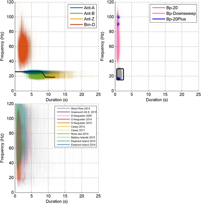
www.nature.com/scientificreports/
Label Call Type References Description
11,27 A constant frequency tone between 28 and 25 Hz (depending on the
Bm-Ant-A Antarctic blue whale unit A
year) without other units
11,27 Antarctic blue whale unit A tone followed by partial or full inter-tone
Bm-Ant-B Antarctic blue whale unit AB
downsweep (unit B)
11,17 Antarctic blue whale ’z-call’ with upper tonal unit A and lower tonal
Bm-Ant-Z Antarctic blue whale z-call; (AKA 3 unit vocalisation)
unit C present (and downswept unit B either present or absent)
Any downswept frequency modulated calls from blue whales. Typically,
11
Bm-D Blue whale FM (AKA D-calls) but not always, longer in duration and lower in frequency than FM
calls from fin and minke whales
12
Bp-20 Hz Fin whale 20 Hz pulse 20 Hz fin whale pulse without substantial energy at higher frequencies
Fin whale 20 Hz pulse with energy at higher frequencies (e.g. 89 or 15,18,24 Fin whale 20 Hz pulse including secondary energy at higher frequen-
Bp-20Plus
99 Hz components) cies (e.g. upper frequency peak near 80–100 Hz)
Frequency modulated, usually downswept calls believed to be pro-
Fin whale FM calls (AKA ‘high frequency’ downsweep; AKA 40 Hz 24,58,59
Bp-Downsweep duced by fin whales. Usually, but not always shorter in duration and
pulse)
slightly higher in frequency than FM calls produced by blue whales
Any transient biological sound that could not be confidently identified
as any of the above classifications. This included sounds that could
potentially be biological, but were substantially different than the above
Unidentified Unidentifiable sounds Not applicable
classifications. It also included FM downsweeps where the analyst
was not certain whether they were blue whale D calls or fin whale
downsweeps
Table 3. Classification and labelling system for blue and fin whale sounds in the SORP library of annotated
recordings.
Unidentified. Detailed descriptions of each of these classifications (including citations) are provided in Table 3,
Figs. 3, and 4. The first two letters of the classification correspond to genus and species, so sounds starting with
Bm were produced by blue whales and Bp by fin whales. The remainder of the classification corresponds to
particular call types for that species (or sub-species in the case of Antarctic blue whales).
In addition to marking the time–frequency boundaries of all potential detections, the analyst also noted
qualitative information about background noise and other sources of sound that were present in each chunk that
was inspected, including the presence and intensity of a “chorus” of elevated background noise in the 20–30 Hz
band over which Antarctic blue whale z calls and fin whale 20 Hz pulses contain most of their energy18,19.
For each site and classification, the 5th and 95th percentile frequency limits and durations of annotations were
measured and plotted to visually identify gross differences among sites as a rough form of “quality control” across
sites and analysts. These percentiles also directly informed respective parameters for automated detectors (Fig. 5).
Signal-to-noise ratio, as described by Lurton (2010)60, was then measured for each manual annotation. In
brief, the root mean square (RMS) signal and noise power, Zs+n, was measured for the full duration of each detec-
tion over the frequency band of interest: 17–29 Hz for Bm-Ant-A, Bm-Ant-B, Bm-Ant-Z; 20–30 Hz for Bp-20 Hz,
Bp-20Plus. Since some analysts marked time–frequency boundaries more tightly than others, a buffer of 1 s before
and after the observation was then created to ensure that no residual signal was included in the measurement of
noise. The noise measurement period was the same duration as the annotation, but split evenly before and after
the buffer (i.e. the noise period was d/2 s before and d/2 s after the
buffer, where d is the duration of the manual
annotation). RMS noise power, Z n and variance of noise power, n2 was measured for t noise over the same band
of interest. Finally, the SNR in dB was calculated as:
(Zs+n − Zn )2
SNR = 20 log10 (1)
�n2
Automated detectors. In order to demonstrate the utility of the annotated library and compare the site-
specific performance of automated detection algorithms, we characterised the performance of two automated
detectors commonly used for detecting sounds of Antarctic blue and fin whales for each of the sites in the
annotated library: an energy sum detector, and a spectrogram correlation detector. Energy sum detectors rely
only on knowledge of the duration and frequency band of the call, so in general can be more flexible if calls are
variable within the band of detection. The spectrogram correlation detectors relies on a priori knowledge of the
shape of the call in the time–frequency domain, and thus perform better when calls are highly stereotyped with
relatively little variation in shape from one call to the next. These two types of detectors were chosen because to
demonstrate that the library was suitable for different types of detectors, and not because we believed they were
optimal for their respective tasks.
For fin whale 20 Hz pulses (both Bp-20 Hz and Bp-20Plus classifications) we applied an energy sum detector38
which targeted the 20 Hz pulse of fin whales by summing the energy for each spectrogram slice in the band
from 15 to 30 Hz. Thus, the detection score was the sum of the squared value of all spectrogram frequency bins
(after noise normalisation) at that time step. In addition to the threshold for summed energy, a minimum and
maximum time over threshold of 0.5 and 2.5 s as well as a minimum time between detections of 0.5 s were used
as criteria for detection of individual fin whale 20 Hz pulses.
Scientific Reports | (2021) 11:806 | https://doi.org/10.1038/s41598-020-78995-8 6
Vol:.(1234567890)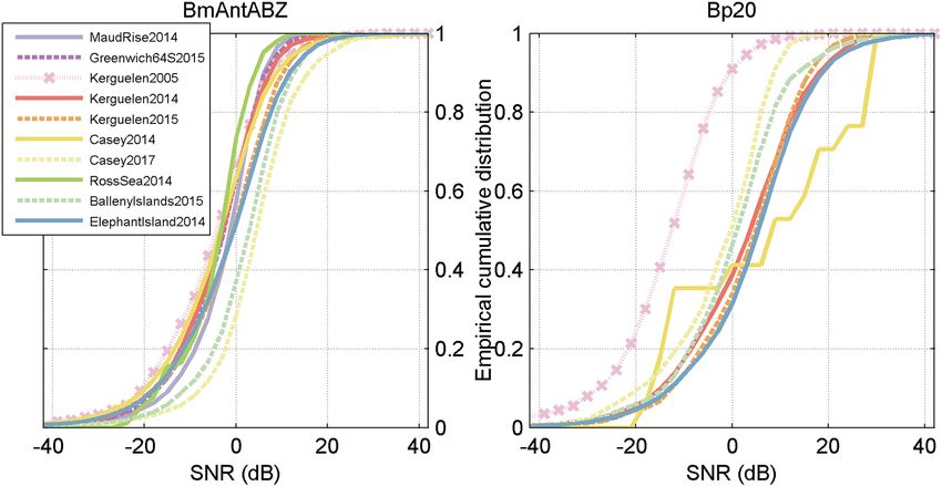
www.nature.com/scientificreports/

                                 Figure 3.  Spectrograms showing examples of Bm-Ant-A (top); Bm-Ant-B (middle); and Bm-Ant-Z (bottom).
                                 All spectrograms used a sample rate of 250 Hz, 256 point FFT with 85% overlap. Bm-Ant-A example is from
                                 site-year Balleny Islands 2015 and starts at 25-Feb 07:24:52. Bm-Ant-B example is from site-year Elephant Island
                                 2014 starting at 20-Jan 19:00:45. Bm-Ant-Z example is from site-year S Kerguelen Plateau 2014 and starts at
                                 01-Mar 12:25:10. Red boxes are indicative of time–frequency boundaries of manual annotations.

Scientific Reports |   (2021) 11:806 |               https://doi.org/10.1038/s41598-020-78995-8                                                 7

                                                                                                                                          Vol.:(0123456789)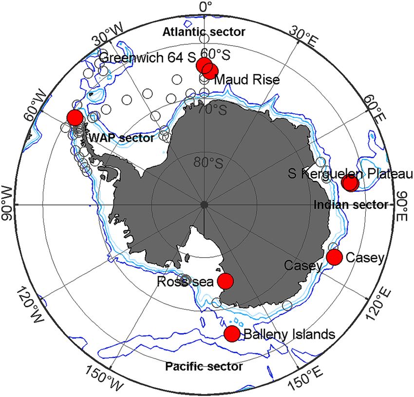
www.nature.com/scientificreports/

                                           Figure 4.  Spectrograms showing Bm-D (top); Bp-Downsweep (middle) and Bp-20 Hz (bottom panel blue box)
                                           along with two forms of Bp-20Plus (bottom panel red and green boxes). All spectrograms in this figure used
                                           a sample rate of 250 Hz, 256 point FFT with 85% overlap. A chorus of blue and fin sounds is visible in the top
                                           and middle panels from 20–30 Hz. Bm-D spectrogram is from S Kerguelen Plateau and starts at 2015-04-16
                                           19:18:00. Bp-Downsweep spectrogram is from S Kerguelen and starts at 2005-04-24 00:05:00. Bp-20 Hz and
                                           Bp-20Plus spectrogram is from Balleny Islands and starts at 2015-03-22 00:50:10.

          Scientific Reports |   (2021) 11:806 |               https://doi.org/10.1038/s41598-020-78995-8                                               8

Vol:.(1234567890)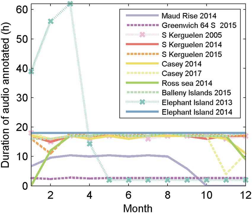
www.nature.com/scientificreports/
Figure 5. Duration (t90%) and frequency bounds (f5% and f95%) of a subset of individual annotations plotted as
99.9% transparent lines. Top left: blue whale sounds for all site-years. Top right: fin whale sounds for all site-
years, excluding ElephantIsland2014 (see “Discussion” for explanation of this exclusion). Black line and black
box show the kernel of the spectrogram correlation detector and time–frequency bounds for the spectrogram
energy-sum detector respectively. For clarity, fin whale 20 Hz with higher frequency components (Bp-20Plus)
are shown as point clouds at the minimum and maximum frequencies rather than vertical lines. Bottom left:
unidentified sounds with colours representing each site.
For Antarctic blue whale song (i.e. classifications of Bm-Ant-A, Bm-Ant-B, and Bm-Ant-Z), we applied a
spectrogram correlation d etector37 which targeted Bm-Ant-Z calls, but was also effective at detecting Bm-Ant-A
and Bm-Ant-B since these call types are essentially each a subset of the full Z-call. The detection score for the
spectrogram cross-correlation detector was the magnitude of the 2D cross-correlation between the correlation
kernel and the spectrogram at each time step. Thus the values for threshold are in a somewhat arbitrary units
of ‘recognition score’ which is the result of cross-correlation between normalised spectrogram and correlation
kernel. In addition to a detection score threshold, a minimum time over threshold and minimum time between
calls were also u sed37.
Detectors were run on the annotated library’s subsets of recordings for each site using Pamguard Version
2.01.0339. Each detector was applied to the subsample of data for each site using a range of thresholds (deter-
mined empirically) in order to create a receiver-operator characteristic (ROC) and precision-recall (PR) curve
for each s ite61,62.
Feature extraction and detector design. The spectrogram correlation and energy sum detectors were parameter-
ised by the time and frequency properties of calls, namely the duration and frequency of each unit of each call.
Scientific Reports | (2021) 11:806 | https://doi.org/10.1038/s41598-020-78995-8 9
Vol.:(0123456789)www.nature.com/scientificreports/
Lower frequency bound (Hz) 15
Upper frequency bound (Hz) 30
Thresholds 0.5, 1, 2, 3, 4, 5, 8, 16, 32, 64
Minimum time over threshold (s) 0.5
Maximum time over threshold (s) 2.5
Minimum time before next detection (s) 1
FFT time resolution (s) 1.024
FFT frequency resolution (Hz) 0.98
Noise normalisation type Average subtraction
Average subtraction: Update constant 0.01
Table 4. Parameters for the energy detector for Bp-20 Hz, Plus.
Unit A duration (s) 8.0
Unit B duration (s) 2
Unit C duration (s) 2
Unit A frequency (Hz) fa (see Eq. 2)
Unit B high frequency fa (see Eq. 2)
Unit B low frequency (Hz) 19.5
Unit C high frequency (Hz) 19.0
Unit C low frequency (Hz) 18.5
Thresholds 20, 40, 80, 160, 320, 640, 1280, 2560, 5120, 10,240
Minimum time over threshold (s) 3
Minimum time before next detection (s) 13
FFT time resolution (s) 1.024
FFT frequency resolution (Hz) 0.98
Noise normalisation type Average subtraction
Average subtraction: update constant 0.001
Table 5. Parameters for the spectrogram correlation detector for Bm-Ant-A,B,Z.
The specific time–frequency properties that we used for each detector were chosen based on published descrip-
tions of calls. The detector parameters were validated by simple comparison with measurements from manual
annotations, specifically the 5th and 95th percentiles of the energy distribution for each annotation (Fig. 5).
The mean duration of all manual annotations for that classification, d , was used to determine the time
boundaries for each automated detection. A “refractory period” of length d was applied after each detection to
prevent new detections from overlapping existing detections. The refractory period prevented multipath arrivals
(e.g. reverberation from the seabed and surface that can arrive before or after the detection) from being detected
by the automated detector. However, the refractory period had the downside of preventing legitimate detection
of calls from different animals that arrived within d seconds of each-other. This was believed to be a prudent
trade-off because multipath arrivals appeared to be far more common than overlapping calls from two differ-
ent animals. Furthermore, by preventing automated detections from overlapping, the total number of possible
automated detections (and true negative/false positive rates) could be calculated from the total duration of the
recording,d , refractory period, and total duration of all the manual annotations.
Noise normalisation was applied to the spectrogram prior to automated detection. The noise normalisation
algorithm was Pamguard’s ‘Average Subtraction’ algorithm, and this involved subtracting a decaying average for
each spectrogram frequency bin at each time step. Specific parameters for the fin whale 20 Hz pulse detector are
described in Table 4 and Antarctic blue whale song in Table 5.
To parameterise the blue whale detector the equation
0.135
fa = 27.6659 − t (2)
365
was used to determine the frequency (in Hz) of unit A of Antarctic blue whale calls. In this equation, derived
from14, fa is the frequency of unit A, and t is the number of days since 12 March 2002. For each site-year t was
set to be the 1 st of June for detector parameters that required estimation of fa.
Scientific Reports | (2021) 11:806 | https://doi.org/10.1038/s41598-020-78995-8 10
Vol:.(1234567890)www.nature.com/scientificreports/
Site-year Ant-A Ant-B Ant-Z Bm-D Bp-20 Bp-20 + BpDownsweep Unidentified
Maud Rise 2014 90.5 (2188) 10.5 (37) 9.5 (28) 5.5 (70) 3.0 (23) 1.0 (5) 2.0 (6) 42.0 (465)
Greenwhich 64
80.5 (827) 47.4 (157) 12.6 (29) 10.5 (66) 1.1 (2) 0.5 (1) 4.7 (46) 57.9 (325)
S 2015
S Kerguelen 2005 59.0 (812) 43.0 (237) 25.0 (166) 25.5 (435) 7.5 (788) 3.0 (78) 17.0 (444) 97.5 (3061)
S Kerguelen 2014 71.0 (2557) 60.5 (1177) 44.0 (563) 33.0 (435) 11.5 (1920) 11.0 (1826) 5.0 (344) 88.0 (4961)
S Kerguelen 2015 60.5 (1970) 49.5 (542) 24.5 (236) 28.5 (1180) 9.0 (552) 6.0 (718) 5.5 (344) 74.0 (1244)
Casey 2014 91.2 (3681) 77.3 (1398) 65.5 (1091) 41.2 (679) 2.1 (17) 0.0 (0) 0.0 (0) 96.9 (5648)
Casey 2017 69.5 (1741) 44.4 (558) 8.6 (119) 38.5 (553) 1.1 (78) 1.1 (214) 0.0 (0) 34.8 (130)
Ross Sea 2014 0.6 (104) 0.0 (0) 0.0 (0) 0.0 (0) 0.0 (0) 0.0 (0) 0.0 (0) 8.5 (255)
Balleny Islands
30.2 (923) 5.9 (44) 2.9 (31) 3.4 (47) 9.3 (951) 1.0 (148) 3.9 (78) 1.5 (18)
2015
Elephant Island
37.4 (2625) 32.0 (1786) 4.7 (152) 7.2 (299) 16.0 (3662) 9.0 (1859) 4.8 (1042) 75.6 (22,927)
2013
Elephant Island
60.5 (6935) 15.5 (967) 2.5 (100) 10.0 (1034) 18.0 (4940) 11.3 (2912) 22.3 (3660) 10.6 (890)
2014
Total 24,363 6903 2515 4798 12,933 7761 5964 39,924
Table 6. Distribution and number of annotations at each site by classification type. Each cell in the table
contains the percentage of hours (with the total number of manual annotations in brackets).
Evaluation of detector performance. Detections from the automated detectors were matched to the human
analyst by comparing the start and end times of all pairs of manual and automated detections. Detections were
considered a match if there was any time overlap between manual and automated observations. This criterion
created the potential for duplicate matches between multiple automated and manual annotations. Duplicates
were identified and labelled, but were neither counted as true positives nor false positives when calculating ROC
and precision-recall curves.
For each threshold automated detections were tabulated to create a confusion matrix of true positives, false
positives, their respective rates, precision, and recall. ROC curves and precision recall curves for each site and
detector were then created from each set of true and false positives (Fig. 7).
To investigate the relationship between the number of automated detections and SNR, a generalised additive
model (GAM)63 was fitted using results from the automated detection process. For each manually detected call,
SNR and whether or not the call was automatically detected was recorded. Specifically, each manual annotation
was assigned a value of 1 when any automated detections matched, and a value of 0 when no automated detec-
tions matched. The matches were modelled as the response of logistic regression with SNR as a predictor using
a GAM with a binomial family error distribution, a logit link function. The GAM was fitted separately for each
site using the default number of knots within the package ‘mgcv’63 in R version 3.6.164.
Results
Distribution of annotations throughout the library. The annotated library consisted of 1880.25 h
(audio duration) of annotated data across 11 site-years and 7 sites. In total, there were 105,161 annotations across
all sites, though the numbers of annotations were neither evenly distributed by site nor classification (Table 6).
Bm-Ant-A was the most numerous annotation with 24,363 manual detections in total, while Bm-Ant-Z was the
least numerous annotation with 2,515 manual detections in total. Ross Sea 2014 had the fewest annotations over
all site-years with only 359 annotations (104 of Bm-Ant-A, and the remainder unidentified). Elephant Island
2014 had the most annotations of all site-years with 21,438 in total including unidentified sounds.
The percentage of hours with each type of annotation was also variable across sites (Table 6). Bm-Ant-A had
the highest percentage across all sites ranging from 0.6 to 91.2% of hours, while Bp-20Plus had the lowest propor-
tions across all sites with no Bp20Plus detections at Casey 2014 or Ross Sea 2014. Antarctic blue whale classifica-
tions were generally present in higher percentage of hours than fin whale sounds across most site-years (Table 6).
Description of classification features. Within each classification the 5th and 95th percentiles of the
frequency bounds and durations were similar across sites, but with a few notable exceptions. Annotations of
Bp-20 Hz, Bp-20Plus, and Bp-Downsweep from Elephant Island 2014, appeared to have longer durations than
these classifications from other sites. However, visual comparison of these annotations suggest that this differ-
ence appeared to arise from the way the analyst marked annotations (i.e. more generous time-boundaries than
other analysts) rather than true difference in the duration of the sound. This suggests that our use of the 90th
percentile energy duration did not provide a measure of duration that was fully robust against analyst variability.
Thus, different features or measures of duration may be more robust or appropriate for developing automated
detectors and/or classifiers.
The stereotyped calls of Antarctic blue whales (Bm-Ant-A, Bm-Ant-B, and Bm-Ant-Z) and those of fin
whales (Bp20Hz, Bp20Plus) are well described in the scientific literature, and are very distinctive from one
another, and this was reflected in the plots of their 90% duration and 5th–95th percentile frequency bounds.
In contrast, the properties of Bm-D and Bp-Downsweep, have not been as well defined in the literature and
Scientific Reports | (2021) 11:806 | https://doi.org/10.1038/s41598-020-78995-8 11
Vol.:(0123456789)www.nature.com/scientificreports/
have forms that appear very similar to each other. Thus these classes have higher potential for confusion and a
higher likelihood of being marked as unidentified. As a result, the time–frequency bounds of unidentified calls
combined two categories: (1) calls that clearly did not fit into any of the defined classifications, and (2) calls that
were intermediate between Bm-D and Bp-Downsweep. However, by restricting annotations to only signals that
can be definitively attributed to one species or the other, they do appear to be distinguishable using duration
and frequency (Fig. 5). This is an instance where having multiple experienced analysts annotate the same data
set might converge on clear guidelines for distinguishing between the two call types. While decisions to only
annotate or detect signals that are clearly attributable to a known species are necessary and justifiable, further
research on acoustic behaviour would be required to determine whether this has downstream implications for
making accurate population abundance estimates.
In contrast to the duration measurements, the upper frequency limit of the Bp-20Plus call type did show
true differences across sites revealing geographic separation similar to that which has been described in previ-
ous studies15,18. Gedamke (2009)15 found that fin whales detected on recorders in the Indian Ocean (including
sites south of 60°S had higher-frequency components near 100 Hz, while fin whales detected in the Tasman Sea
(Pacific Ocean including sites south of 60° S) had higher frequency components at 82 and 94 Hz. Širović et al.
(2009)18 found that fin whale sounds recorded off the WAP and Scotia Sea had higher frequency components
around 90 Hz, while recordings off East Antarctica had higher frequency components near 100 Hz. In our study,
the Indian and Atlantic sectors had higher frequency components around 100 Hz, while the WAP and Pacific
sectors were around 90 Hz. Recordings investigated by Gedamke (2009)15 and Širović et al. (2009)18 were made
from 2003 to 2007, whereas all but one of our recordings were made in 2013–2017. Thus, there appears to be
decadal-scale stability in the broad geographic distribution and form of these sounds.
Temporal distribution of annotations within a site‑year. In general there were more annotations
from Feb through May (late summer through autumn) than in other months, though there were a number of
exceptions to this general trend (Fig. 6). Bm-Ant-A had maximum number of annotations from June–August
at Elephant Island 2014 and Kerguelen 2014. Bm-Ant-Z also peaked in July at Kerguelen 2014. At Casey 2014
Bm-D had a maximum in December, while at Elephant Island 2014 Bm-D had maximum monthly annotations
in October. At Elephant Island 2014 Bp-Downsweep had a maximum in January.
While there is a temptation to speculate on the drivers of these temporal trends, such analyses are beyond
the scope of this work, which was the creation of a dataset suitable for characterising automated detectors.
Rather, the purpose of plotting monthly number of annotations by site is simply to describe the contents of the
Annotated Library and to identify months or seasons that do and do not have sufficient number of detections
to allow characterisation of a detector. In that regard, there is a notable lack of fin whale annotations (Bp-20 Hz,
Bp-20Plus, and Bp-Downsweep) from July-December.
An example of using the annotated data to examine the performance of automated detec-
tors. ROC, precision‑recall, and SNR. ROC and PR curves indicated that detector performance was fair-to-
poor for these datasets. ROC and PR curves varied by site for both blue and fin whale detectors with some sites
much worse than others (Fig. 7). For example, the true positive rate for the blue whale detector ranged from 8
to 55% at a false alarm rate of 1% (~ 2.8 false positives per hour). The true positive rate for the fin whale detector
ranged from 1 to 76% at a false alarm rate of 1% (~ 14.4 false positives per hour).
In addition to variability in detector performance, the distribution of SNR also varied across sites with the
combined Bp20 and Bp20 plus distributions showing more variability than the combined Bm-Ant-A, Bm-Ant-B,
and Bm-Ant-Z distributions (Fig. 8). The modelled probability of detection at 1% false positive rate was similar
across sites at high-SNR, but was more variable across sites at low SNR (e.g. < 0 dB) (Fig. 9).
Discussion
We created an annotated library of blue and fin whale sounds that spans four circumpolar Antarctic recording
regions, five different years (2005, 2013, 2014, 2015, 2017), and five different types of instrument. The acoustic
data in our library come from a variety of different data collection campaigns conducted by laboratories from
five nations.
The distribution of calls in our library varied considerably across sites, years, and species. Antarctic blue
whale sounds, particularly Bm-Ant-A, were the most numerous, and are well represented at all sites, and over
most times throughout the year. Fin whale sounds had a much more seasonal representation in the annotated
library with annotations in late summer and throughout autumn months, and few throughout the rest of the year.
Fin whale Bp-20Plus sounds also revealed some degree of biogeographic separation with calls in the Atlantic
and Indian sectors having higher upper-frequency components than those in the Pacific and WAP sectors. The
annotations in the library form a representative ground-truth dataset that can be used to extract the features of
each call type, and also to train and characterise the performance of automated detectors.
Detector performance. To test the utility of the library, we characterised the performance of a spectro-
gram correlation detector for blue whale calls and an energy sum detector for fin whale calls. The performance
of the automated detectors varied by site-year. Neither detector performed particularly well, and some sites and
years showed much worse performance than others (Fig. 7). Differences in detector performance broadly fol-
lowed differences in SNR across sites such that sites with lower SNR had worse performance than those with
higher SNR (Fig. 8). Across sites, the automated detectors showed greater variability at low SNR than at high
SNR (Fig. 9).
Scientific Reports | (2021) 11:806 | https://doi.org/10.1038/s41598-020-78995-8 12
Vol:.(1234567890)www.nature.com/scientificreports/
Figure 6. Rate of annotations per season for each site and sound type. Rate is calculated as the total number
of annotations in that season divided by the total effort (in hours) for that season. Antarctic blue whale tonal-
sounds are in the left column. Fin whale 20 Hz pulses are in the middle column. Blue D, fin downsweeps, and
unidentified calls are in the third column. Vertical scale may differ for each panel.
Characterising the performance of an automated detector and estimating the probability of automatic detec-
tion as a function of SNR using a representative subset of data, as we have done here, can be important steps
towards meaningful comparisons of animal sounds across sites and over time43,46. In addition to performance
of the detector, differences in call density (a useful metric for such comparisons) can arise from site-specific fac-
tors such as differences in instrumentation (including depth)54, analyst v ariability53,65, ambient and local noise
sources36,66, propagation46,67, and animal b ehaviour43. These factors are not mutually exclusive, and can interact
in a complex manner. Addressing and accounting for how each of these factors affects the call density is beyond
the scope of this manuscript, but is a requirement if one wants to make comparisons of acoustic detections that
meaningfully address biological questions of distribution and temporal trends. The library and methods we
present here for assessing the performance of the detectors are a step away from estimating call-density, which
in turn is a step away from estimating animal d ensity68.
None of the passive acoustic studies of Antarctic blue or fin whales to date (listed in Table 1) have completely
reported on the performance of their detector over a representative subsample of their data. The methods we have
presented here for characterising the performance of a detector on a representative subsample of data constitute
a bare minimum of reporting for future studies that utilise automated detectors to study Antarctic blue and fin
whale calls. Specifically, reporting should include all parameters for the automated detector including any noise
Scientific Reports | (2021) 11:806 | https://doi.org/10.1038/s41598-020-78995-8 13
Vol.:(0123456789)www.nature.com/scientificreports/
Figure 7. ROC curves (top), and precision-recall curves (bottom) for Bm-Ant-A; Bm-Ant-B; Bm-Ant-Z
spectrogram correlation detector (left) and Bp-20 energy detector (right). Sites with fewer than 30 detections of
Bp20 (Maud Rise 2014, Greenwich64S 2015, Casey 2014, Ross sea 2014) are not shown.
pre-processing steps; distribution and SNR of ground-truth detections throughout the dataset; and true and false
positive rates and/or precision and recall of the detector for a representative sample of the data.
We hope the open-access annotated library we have presented here can provide a base dataset upon which
to develop improved detectors i.e. with higher true positive rates and lower false positive rates. Here we have
extracted duration and frequency measurements from annotations, but the library can readily be used to extract
more complex features such as pitch-tracks69 or other time–frequency features70 to train machine learning
algorithms37,71,72, deep neural networks73, or other any other advanced detectors that may provide better perfor-
mance than the spectrogram correlation detector. Better detectors would not only reduce a source of uncertainty
in estimating call-density, but would also reduce the amount of analyst effort required to verify true positives
and account for false positives.
Future development of this dataset will aim to expand the annotated library to serve as a test-bed for subse-
quent analyses that address the issues of noise, detection range, and analyst variability to produce standardised
outputs that are appropriate for circumpolar comparisons of call-density. This additional development would
entail (1) collating pressure calibration details for noise analysis at each site-year, (2) estimating detection range
throughout each site-year and (3) having multiple analysts annotate the same subsets of data for the purposes
of quantifying analyst bias and variability.
Scientific Reports | (2021) 11:806 | https://doi.org/10.1038/s41598-020-78995-8 14
Vol:.(1234567890)www.nature.com/scientificreports/
Figure 8. Empirical cumulative distribution of signal-to-noise ratio (SNR) of manually annotated blue whale
song (left) and manually annotated fin whale pulses (right) for each site. Blue whale distributions include calls
classified as Bm-Ant-A, Bm-Ant-B, or Bm-Ant-Z. Fin whale distributions includes calls classified as Bp-20 Hz
or Bp-20Plus.
Figure 9. Probability of automated detection of annotated call as a function of SNR. Specifically, these are the
marginal effects for SNR from the binomial GAM from Eq. (3). Left: blue whale annotations (any of Bm-Ant-A,
Bm-Ant-B, Bm-Ant-Z) for the spectrogram correlation detector using the theshold nearest to false positive rate
of 0.01. Right: Bp-20 annotations (either Bp-20 Hz or Bp-20Plus) for the energy sum detector with the threshold
nearest to false positive rate of 0.01. Shading shows 95% confidence intervals for each site, and rug plots show
the distribution of data as.
Conclusions
We created an annotated library of blue and fin whale sounds that spans four circumpolar Antarctic recording
regions, five different years (2005, 2013, 2014, 2015, 2017), and five different types of instrument. The annotations
in the library form a representative ground-truth dataset and we demonstrate how to train, test, and characterise
the performance of two common automated detectors using the library. The annotated library we present here
can serve as a benchmark upon which detectors can be developed, compared, and improved upon. It may also
serve as a base dataset to develop additional analytical techniques to enable robust comparisons of acoustic
detections of blue and fin whale across diverse circumpolar sites and over long spans of time.
We encourage further contributions of data and annotations to help expand the library, and in the future hope
to include annotations of sounds from additional Antarctic species, as well as data from other recording locations
Scientific Reports | (2021) 11:806 | https://doi.org/10.1038/s41598-020-78995-8 15
Vol.:(0123456789)www.nature.com/scientificreports/
throughout the southern hemisphere. The IWC-SORP/SOOS Acoustic Trends Annotated Library is freely avail-
able from http://data.aad.gov.au/metadata/records/AcousticTrends_BlueFinLibrary74. The larger datasets from
which the Annotated Library was derived are available under the data sharing provisions of the Antarctic Treaty
(1959), and these can be requested by contacting the authors and/or institutions that hold these data.
Code availability
Code available in the IWC-SORP/SOOS Annotated Library (https: //data.aad.gov.au/metada ta/record
s/fulldi spla
y/AcousticTrends_BlueFinLibrary).
Data availability
Data used in this study are publicly available under a Creative Commons 4.0 Attribution licence. They can
be accessed via the Australian Antarctic Data Centre at http://data.aad.gov.au/metadata/records/AcousticTr
ends_BlueFinLibrary.
Received: 15 April 2020; Accepted: 2 December 2020
References
1. Mellinger, D. K., Stafford, K. M., Moore, S. E., Dziak, R. P. & Matsumoto, H. An overview of fixed passive acoustic observation
methods for cetaceans. Oceanography 20, 36–45 (2007).
2. Van Parijs, S. et al. Management and research applications of real-time and archival passive acoustic sensors over varying temporal
and spatial scales. Mar. Ecol. Prog. Ser. 395, 21–36 (2009).
3. Sousa-Lima, R. S., Norris, T. F., Oswald, J. N. & Fernandes, D. P. A review and inventory of fixed autonomous recorders for passive
acoustic monitoring of marine mammals. Aquat. Mamm. 39, (2013).
4. Van Opzeeland, I. et al. Towards collective circum-Antarctic passive acoustic monitoring: The Southern Ocean Hydrophone
Network (SOHN). Polarforschung 83, 47–61 (2013).
5. Branch, T. A., Matsuoka, K. & Miyashita, T. Evidence for increases in Antarctic blue whales based on Bayesian modelling. Mar.
Mammal Sci. 20, 726–754 (2004).
6. Branch, T. A. Abundance of Antarctic blue whales south of 60 S from three complete circumpolar sets of surveys. J. Cetacean Res.
Manag. 9, 253–262 (2007).
7. Rocha, R. C. Jr., Clapham, P. J. & Ivashchenko, Y. Emptying the oceans: A summary of industrial whaling catches in the 20th
century. Mar. Fish. Rev. 76, 37–48 (2015).
8. Branch, T. A. & Butterworth, D. S. Estimates of abundance south of 60° S for cetacean species sighted frequently on the 1978/79
to 1997/98 IWC/IDCR-SOWER sighting surveys. J. Cetacean Res. Manag. 3, 251–270 (2001).
9. Cooke, J. G. Balaenoptera musculus ssp. intermedia. IUCN Red List Threat. Species e.T41713A50226962 (2018). https://doi.
org/10.2305/IUCN.UK.2018-2.RLTS.T41713A50226962.en.
10. Sears, R., Ramp, C., Douglas, A. & Calambokidis, J. Reproductive parameters of eastern North Pacific blue whales Balaenoptera
musculus. Endanger. Species Res. 22, 23–31 (2013).
11. Rankin, S., Ljungblad, D. K., Clark, C. W. & Kato, H. Vocalisations of Antarctic blue whales, Balaenoptera musculus intermedia,
recorded during the 2001/2002 and 2002/2003 IWC/SOWER circumpolar cruises, Area V Antarctica. J. Cetacean Res. Manag. 7,
13–20 (2005).
12. Watkins, W. A., Tyack, P., Moore, K. E. & Bird, J. E. The 20-Hz signals of finback whales (Balaenoptera physalus). J. Acoust. Soc.
Am. 82, 1901–1912 (1987).
13. McDonald, M. A., Mesnick, S. L. & Hildebrand, J. A. Biogeographic characterisation of blue whale song worldwide: using song to
identify populations. J. Cetacean Res. Manag. 8, 55–65 (2006).
14. Gavrilov, A. N., McCauley, R. D. & Gedamke, J. Steady inter and intra-annual decrease in the vocalization frequency of Antarctic
blue whales. J. Acoust. Soc. Am. 131, 4476–4480 (2012).
15. Gedamke, J. Geographic variation in Southern Ocean fin whale song. Submitt. to Sci. Comm. Int. Whal. Comm. SC/61/SH16, 1–8
(2009).
16. Shabangu, F. W., Yemane, D., Stafford, K. M., Ensor, P. & Findlay, K. P. Modelling the effects of environmental conditions on the
acoustic occurrence and behaviour of Antarctic blue whales. PLoS ONE 12, e0172705 (2017).
17. Širović, A. et al. Seasonality of blue and fin whale calls and the influence of sea ice in the Western Antarctic Peninsula. Deep Sea
Res. Part II Top. Stud. Oceanogr. 51, 2327–2344 (2004).
18. Širović, A., Hildebrand, J. A., Wiggins, S. M. & Thiele, D. Blue and fin whale acoustic presence around Antarctica during 2003 and
2004. Mar. Mammal Sci. 25, 125–136 (2009).
19. Thomisch, K. et al. Spatio-temporal patterns in acoustic presence and distribution of Antarctic blue whales Balaenoptera musculus
intermedia in the Weddell Sea. Endanger. Species Res. 30, 239–253 (2016).
20. Tripovich, J. S. et al. Temporal segregation of the Australian and Antarctic blue whale call types (Balaenoptera musculus spp.). J.
Mammal. 1–8 (2015). https://doi.org/10.1093/jmammal/gyv065.
21. Dréo, R., Bouffaut, L., Leroy, E., Barruol, G. & Samaran, F. Baleen whale distribution and seasonal occurrence revealed by an ocean
bottom seismometer network in the Western Indian Ocean. Deep. Res. Part II Top. Stud. Oceanogr. 161, 132–144 (2019).
22. Bouffaut, L., Madhusudhana, S., Labat, V., Boudraa, A.-O. & Klinck, H. A performance comparison of tonal detectors for low-
frequency vocalizations of Antarctic blue whales. J. Acoust. Soc. Am. 147, 260–266 (2020).
23. Bouffaut, L., Dréo, R., Labat, V., Boudraa, A.-O. & Barruol, G. Passive stochastic matched filter for Antarctic blue whale call detec-
tion. J. Acoust. Soc. Am. 144, 955–965 (2018).
24. Gedamke, J. & Robinson, S. M. Acoustic survey for marine mammal occurrence and distribution off East Antarctica (30–80°E)
in January-February 2006. Deep Sea Res. Part II Top. Stud. Oceanogr. 57, 968–981 (2010).
25. Gedamke, J., Gales, N., Hildebrand, J. A. & Wiggins, S. Seasonal occurrence of low frequency whale vocalisations across eastern
Antarctic and southern Australian waters, February 2004 to February 2007. Rep. SC/59/SH5 Submitt. to Sci. Comm. Int. Whal.
Comm. Anchorage, Alaska SC/59, 1–11 (2007).
26. Leroy, E. C., Samaran, F., Bonnel, J. & Royer, J. Seasonal and diel vocalization patterns of Antarctic blue whale (Balaenoptera
musculus intermedia) in the Southern Indian Ocean: a multi-year and multi-site study. PLoS ONE 11, e0163587 (2016).
27. Miller, B. S. et al. Validating the reliability of passive acoustic localisation: a novel method for encountering rare and remote
Antarctic blue whales. Endanger. Species Res. 26, 257–269 (2015).
28. Miller, B. S. et al. Software for real-time localization of baleen whale calls using directional sonobuoys: A case study on Antarctic
blue whales. J. Acoust. Soc. Am. 139, EL83–EL89 (2016).
Scientific Reports | (2021) 11:806 | https://doi.org/10.1038/s41598-020-78995-8 16
Vol:.(1234567890)You can also read