Income Changes Do Not Influence Political Participation: Evidence from Comparative Panel Data - Sebastian Jungkunz Paul Marx
←
→
Page content transcription
If your browser does not render page correctly, please read the page content below
Sebastian Jungkunz
Paul Marx
Income Changes Do
Not Influence Political
Participation: Evidence from
Comparative Panel Data

                        uni-due.de/soziooekonomie/wp

        ifso working paper                         2021
                                                    2019 no.11
                                                          no.5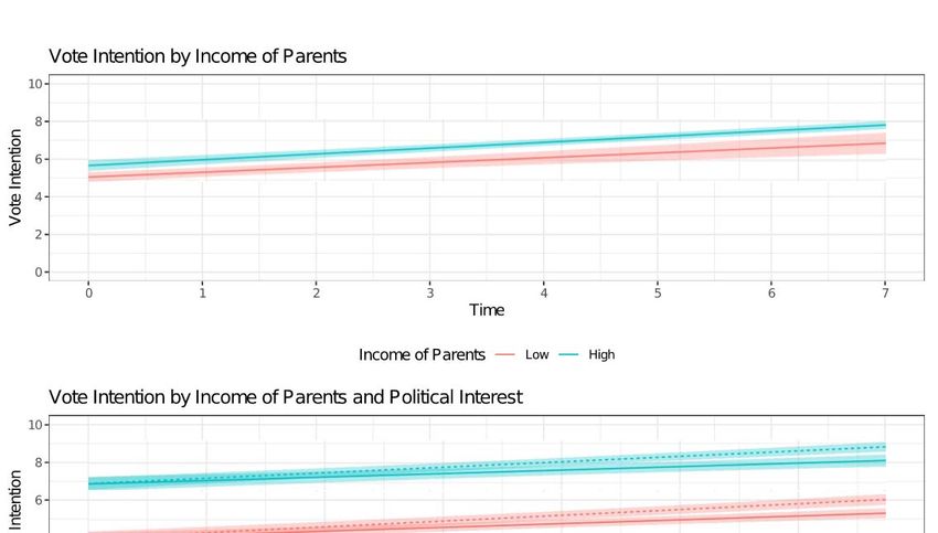
Income changes do not influence political participation.
                    Evidence from comparative panel data

                                    Sebastian Jungkunza
          University of Duisburg-Essen, University of Bamberg, Zeppelin University

                                         Paul Marx
             University of Duisburg-Essen, University of Southern Denmark, IZA

Abstract
The income gradient in political participation is a widely accepted stylized fact. This article
asks how income effects on political involvement unfold over time. Using nine panel datasets
from six countries, it analyzes whether income changes have short-term effects on political
involvement, whether effects vary across the life-cycle, and whether parental income has an
independent influence. Irrespective of indicator, specification, and method (hybrid models,
inclusion of lags and leads, error-correction models), we find neither significant short-term
effects of income changes nor life-cycle variation in these effects. However, parental income
does seem to affect political socialization. Descriptive evidence and latent-growth-curve
modeling based on household panels show that participatory inequality by parental income is
already large before voting age. Poorer voters do not catch up with their richer peers in their
twenties. This implies an urgent need for research on (political) inequality in youth and
childhood.

Keywords
Participation, political inequality, panel data, socialization, income

Funding information
This research is part of the project “The influence of socio-economic problems on political
integration” (PI: Paul Marx) funded by the North Rhine-Westphalian Ministry of Culture and
Science.

a
 Corresponding author
University of Duisburg-Essen
Institute for Socio-Economics
Lotharstr. 65
DE-47057 Duisburg
sebastian.jungkunz@uni-due.de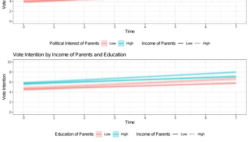
Introduction
The income gradient in political participation is an important research topic and a pressing
societal concern. A large literature has reported lower political involvement among voters
with low income or other socio-economic problems (Aytaç et al. 2020; Erikson 2015; Dalton
2017; Gallego 2015; Lawless & Fox 2001; Marx & Nguyen 2018; Pacheco & Plutzer 2008;
Solt 2008; Schlozman et al. 2012).
Although the underlying theoretical models differ, studies often assume that low income
triggers social and psychological mechanisms that situationally inhibit political involvement
(e.g., Rosenstone 1982).1 However, recent scholarship has started addressing the related
questions of whether income effects on political involvement are causal and how these effects
unfold over time (Margalit 2019; Prior 2019). Based on the observation that political
participation often becomes habitual with age and therefore resilient to external influences
(Plutzer 2002), an emerging literature places economic hardship in the life-cycle (Akee et al.
2020; Emmenegger et al. 2017; Ojeda 2018; Prior 2019). A key implication is that cross-
sectional income gaps tend to be confounded with previous experiences and, hence, do not
reflect a direct causal effect. That said, the underlying theoretical arguments differ in
important ways and the associated empirical evidence remains patchy. Moreover,
experimental research outside political science has documented impressive short-term effects
of economic scarcity on mental capacities (Haushofer & Fehr 2014; Mani et al. 2013;
Schilbach et al. 2016; Vohs 2013) that are also crucial for political involvement (Denny &
Doyle 2008; Fowler & Kam 2006; Holbein & Hillygus 2020; Ojeda & Pacheco 2019).
Although this research has not yet been linked explicitly to political participation, it suggests
that income changes could indeed have immediate effects on participation.
In sum, the question of whether short-term changes in income (or socio-economic position in
general) are able to trigger short-term reactions in political involvement is theoretically
ambiguous and still awaits comprehensive empirical assessment. A problem in the existing
literature is that the few longitudinal studies typically rely on just one dataset (and rarely more
than three). Given the idiosyncratic features of some panel datasets and contexts, this provides
a weak basis for knowledge accumulation. We therefore analyze income changes in nine
panel datasets from six countries (Germany, Netherlands, Spain, Switzerland, UK, USA).
While all advanced capitalist democracies, these countries do provide reasonable variation in
socio-economic patterns and political institutions. Consistent findings in this group, hence, are
likely to be generalizable to Western democracies. We also wish to highlight this study’s
achievements in identifying a comparatively large number of panel datasets with political
information as an independent contribution to political behavior research.
Our analysis of individual income trajectories, by far the most comprehensive of its kind,
produces an important insight that is applicable across all contexts. Irrespective of method and
operationalization, income changes have hardly any predictive power for short-term changes
in the propensity to participate in politics. This holds for reported voting or voting intentions

1
  We use “political involvement” as an overarching concept capturing individuals’ propensity to cognitively,
emotionally, or behaviorally engage with politics. This helps us to summarize results and literature based on
diverse indicators, such political interest, efficacy, or participation. When we discuss specific results, we do so
with reference to the precise indicator.

                                                                                                                 1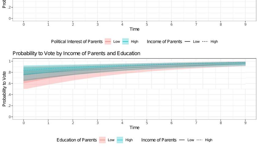
as well as for attitudinal measures of political involvement. It is also robust to different ways
of measuring income changes.
How can we make sense of this nonfinding? As mentioned above, some studies have
explained the socio-economic gradient in participation with political habits that already
emerge during socialization. Most prominently, Schlozman et al. (2012: 177) suggested that
parental influences contribute to pronounced participatory inequality “at the starting line” of
voting age. Hence, cross-sectional income gaps might reflect an early influence of parental
income on political socialization that crystalizes into stable patterns of involvement or apathy.
While a full treatment of this conjecture is beyond the scope of this article, we provide a first
assessment based on two analyses. First, by merging parents and children in household panels
in four countries, we descriptively show that “inequality at the starting line” is a generalizable
phenomenon. Moreover, we observe that children from poorer families typically do not catch
up in their twenties. Second, a latent-growth-curve analysis in the United Kingdom adds
nuance to this picture. The multivariate analysis confirms that parental socio-economic status
influences the starting level and development of political participation. However, parental
education and political interest appear to be more relevant in determining socialization
patterns. This shows the need to unpack parental socio-economic background into different
components.
In sum, our analyses yield key insights into unequal political participation. While short-term
income dynamics do not influence political involvement, youth and childhood experiences are
a key source of inequality. We hence point to the urgent need for future research on socio-
economic problems during these life stages.

Theoretical arguments: Income, voting, and the political life-cycle
By now, there should be little doubt that income correlates with political participation and that
the poor in particular tend to abstain from voting. Yet, research has not conclusively answered
whether we can think of this link as causal and how causality may operate (Akee et al. 2020).
These questions are inseparable from the question of how income effects unfold over time.
Three possibilities appear likely.2
First, income might be seen as a summary indicator of background factors unfavorable to
political participation (Pacheco & Plutzer 2008). Income could relate to differences in, inter
alia, health, housing conditions, education, class background, quality of social relationships,
experiences of discrimination, ethnicity, personality, values, civic skills, or cognitive ability.
In most cases, the effects of such background factors are likely to be cumulative and to
contribute to a rather stable disposition to abstain or participate. To the extent that the income-
participation link is “spurious” and really caused by these background factors, year-to-year
fluctuations in income should have no short-term impact on political participation.

2
  We restrict the discussion to theoretical explanations relating to voters’ individual situation. There is an
additional literature linking participatory inequality to political elites and communication (Leighley & Nagler
2013; Marx & Nguyen 2018; Piven & Cloward 1988; Solt 2008). While the temporality of these mechanisms is
far from obvious, they provide an alternative possibility to theorize dynamic links between income and
participation.

                                                                                                             2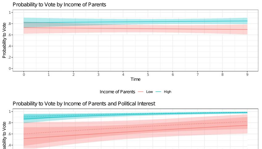
Second, income could be directly causally related to participation. This would be the case if
socio-economic problems create cognitive “opportunity costs” for engagement with politics,
as argued by Rosenstone (1982) or Brody & Sniderman (1977). Going even further, several
studies from psychology and behavioral economics have demonstrated that situational
economic scarcity immediately impairs mental capacities through stress, cognitive load, and
ego depletion (Haushofer & Fehr 2014; Mani et al. 2013; Schilbach et al. 2016; Vohs 2013).
Short-term changes in income then could be decisive for how much time and attention
potential voters allocate to politics, how easy they find it to process and recall political
information, and how efficacious they feel (Marx & Nguyen 2018). If such effects are strong
enough, they might situationally influence for example whether habitual political involvement
is translated into actual voting (Holbein & Hillygus 2020).
Third, income might only have a direct causal effect at certain stages of the life-course.
According to the “impressionable years” hypothesis, political behaviors and orientations are
comparatively malleable until early adulthood and become increasingly resilient afterwards
(Dinas 2013; Stoker & Jennings 2008). Accordingly, economic shocks could have more
immediate effects at young ages but lose explanatory power during habituation (Emmenegger
et al. 2017; Hassell & Settle 2017). Another possibility, linked to an even earlier life-cycle
stage, is that socio-economic factors operate through parental transmission during youth and
childhood (Akee et al. 2020; Schlozman et al. 2012: 177-198). Although studies rarely make
explicit links to income effects (an important exception is Ojeda 2018), several do confirm
that political inequality is a) already large at voting age and b) strongly influenced by parental
characteristics (Cesarini et al. 2014; Jennings et al. 2009; Plutzer 2002; Prior 2019). To the
extent that adults’ current income and participatory inclination are jointly influenced by early
(and, hence, typically unobserved) socio-economic experiences, income gaps in political
behavior would be inflated in cross-sectional data.

State of existing research on the temporality of income effects
We are not the first to study the temporal dimension of the link between socio-economic
hardship and political involvement. A number of recent studies have explicitly addressed the
issue. Emmenegger et al. (2017) argued and showed with difference-in-difference matching
based on German panel data a) that unemployment only depresses political interest during the
impressionable years of early adulthood and b) that the negative effect of youth
unemployment on interest and turnout lasts well into prime age. This confirms the suspicion
that people’s resilience to economic shocks grows over the life cycle and that present socio-
economic variables can be biased by earlier experiences. However, Emmenegger et al. (2017)
did not consider parental background as a preceding influence.
Ojeda (2018) goes in a similar direction, but his theory differs in crucial ways. He argued that
family income during childhood influences turnout inequality at young age. The relevance of
family background is crowded out by the effect of personal (current) income as people get
older. This implies that current income should have direct and more or less immediate effects,
at least from prime age onwards—which is the opposite of what Emmenegger and colleagues
argued. Unfortunately, the empirical results are impossible to compare because Ojeda largely
relied on age-income interactions in cross-sectional data and because the dependent variables

                                                                                                3
and countries differed. Moreover, Ojeda’s random-effects estimators cannot be used to isolate
short-term variability, because they do not decompose within- and between-variation.
Nonetheless, a key insight of Ojeda’s study (which we follow in the second part of the paper)
is that socio-economic family background should be modeled explicitly, in particular
regarding young citizens.
Closely related to our work, but with a narrower focus on political interest, is Prior’s (2019)
comprehensive study. He used fixed-effects and first-difference models with distributed lags
based on British, German, and Swiss panel data to show that income changes have no
systematic influence on political interest (chapter 12). This is true for year-to-year fluctuations
and two-year long-run effects. Although he separately demonstrated that children are strongly
influenced by parents’ political interest (chapter 11) and education (chapter 8), he did not
explicitly address the influence of parental income on young voters’ political involvement.
According to Ojeda’s (2018) reasoning, he hence missed one potential channel through which
income might matter. Crucially, we also do not know whether Prior’s results hold for other
dependent variables than political interest.
Lahtinen et al. (2019) used Finnish register data and a sibling design to isolate effects of
family characteristics on voting turnout. While they found strong effects of socio-economic
background and of parents’ voting in an earlier election, socio-economic background largely
seemed to matter in the form of parental education and occupation. Parental income had a
significant but small effect. This suggests that the effects of parental income should not be
taken at face value (as in Ojeda 2018) when other parental characteristics are not controlled
for. Support for this conclusion comes from the natural experiment of comparing adopted and
biological children in Cesarini et al. (2014), which suggests that parental-income effects are
partly attributable to prebirth factors. However, another natural experiment recently
confirmed that positive income shocks for children from low-income families can have lasting
positive effects on voting if they occur early in the life course (Akee et al. 2020).
Research questions
In sum, income effects on political participation are a broadly studied topic. The literature has
only recently sought to causally understand this link by studying its temporal ordering. To
date, the literature is far from conclusive. Studies on the topic have often considered
individual cases and do not always build on each other; they thus provide little knowledge
accumulation. Consequently, we lack clear theoretical and empirical knowledge on whether
income gaps are causal and how they unfold over time. Many studies have indicated life-cycle
variation, but we know little about a) how much short-term variability remains after the
“impressionable years,” b) how strong the influence of parental socio-economic status is, and
c) which aspect of parental socio-economic status might matter. In our view, these knowledge
gaps lead to three pressing research questions (RQ):
RQ1: Do income changes trigger short-term effects on political involvement?
RQ2: Do income effects on political involvement vary across the life cycle?
RQ3: How strong is the influence of parental income on the starting level and development of
political involvement?
4In some cases, it would be possible to formulate concrete hypotheses. For example, an
opportunity-cost hypothesis would predict negative short-term effects of personal income
drops. An impressionable-years hypothesis would predict that these effects are restricted to
early adulthood, while a two-income-gaps hypothesis (based on Ojeda 2018) would restrict
them to prime age and later years. The latter would overlap with a starting-line hypothesis in
predicting early participatory inequality by parental income. As these examples illustrate,
existing research allows a large number of nuanced but partly contradictory hypotheses. It
also leaves some aspects under-theorized such as the influence of parental income on the
development of political involvement. Against this background, we believe that the
formulation of open research questions is more appropriate at this stage.
Research strategy
Addressing the research questions requires individual panel data. In an ideal situation, we
would base our analysis on panels that a) are large enough to have a sufficient number of
respondents in different income and age groups; b) sample households so that parental
influences can be modelled explicitly; c) stem from different countries to allow for
generalizable statements. Panels that fulfill criteria a) and b) and consistently include political
dependent variables over time are rare. By screening several international studies, we
identified nine panels from six countries that fulfilled our criteria to different degrees (Table
1). Unfortunately, we had to exclude a number of high-quality datasets that did not
sufficiently cover politics (for instance, the “Household, Income and Labour Dynamics in
Australia Survey”). That said, we have used a substantially larger number of datasets than
comparable studies. We see this as an independent contribution beyond our concrete research
findings. With data from Germany, Netherlands, Spain, Switzerland, UK, and the United
States we can study income effects in diverse contexts. The included countries differ, for
instance, in their party systems, welfare-state generosity, and levels of income inequality and
unemployment. If the relationship between income and political involvement is similar across
these contexts, it can be assumed to be a general feature of advanced capitalist democracies.
As already stressed, we know little about the precise temporal logic through which income
effects on political involvement unfold. This is a theoretical lacuna, but it matters for
methodological choices, because modeling strategies entail different assumptions about
underlying dynamics. In any case, answering RQ1 requires us to decompose within-person
changes over time and inter-individual changes. If political involvement is largely explained
by cross-sectional income differences and unresponsive to income changes, we would have to
conclude that any link is likely driven by spurious correlations (which would arise if personal
income and involvement are influenced by family background, for instance). Effects due to
changes within respondents can usually be isolated with fixed-effects (FE) estimation. We
prefer hybrid models (Bell & Jones 2015), because they allow an explicit comparison of
within- and between-estimators. The model has the form
(1)
5where the political involvement of individual i in period t (POLit) is a function of income
(changes). β1 indicates the effect of (time-variant) income (INCit) after a de-meaning
transformation. This within-effect is identical to an FE model (Bell and Jones 2015) and
hence does not suffer from heterogeneity bias. β3 is the between-effect of the (time-constant)
intra-personal mean income ( ), which might be inflated by such bias. While the within-
effect shows how changes of income within a person’s lifetime are related to political
participation, the between-effect shows whether those who have always earned more are also
those who were always more politically involved. β2 and β5 are the effects of additional time-
variant and time-invariant predictors xit and zi.
A key advantage of hybrid models is that they are relatively undemanding in terms of data
structure. Because they only require information about political involvement and income over
few waves, we could include all datasets in Table 1. An important downside pertains to the
modelling of the underlying dynamics, which is restrictive and not necessarily realistic. The
model in Equation 1 assumes that income changes between t1 and t2 fully exert their effect at
t2. Yet, this might not be the case if changes in political involvement predate income changes
or follow them with a delay. For instance, income changes may be anticipated or influence
political habits slowly. To account for these possibilities, we ran additional FE models
including lag and lead variables, which would pick up any preceding or delayed effect:
(2)
The model, which includes individual FE αi, and time-varying control variables zit captures
the effect of income changes up to three years after (β2, β3, β4) and a year before (β5) they
occur. The more lags and leads of income are included, the more informative the model.
However, the number is limited by the need to observe enough panelists with a sufficient
number of subsequent waves. We pragmatically chose a specification with three-year lags of
INCit and a one-year lead (assuming that income changes are rarely anticipated far into the
future). This reduced the number of datasets we could include in the analysis (Table 1). Note
that the model in Equation 2 can be estimated with income as a continuous variable and in the
form of a binary “shock” variable (the operationalization is discussed below). The latter is
useful to assess how relatively large income drops (as opposed to gradual changes) influence
political involvement as discrete events. It also avoids the assumption that positive and
negative changes have uniform effects.
An alternative way to model dynamic links between income and political involvement is
provided by error correction models (ECMs), which are particularly useful for capturing
effects distributed over several periods (De Boef & Keele 2008; Prior 2019). We included
these models as robustness checks. Taken together, the three analytical strategies should be
sufficiently flexible to capture various temporal dynamics through which income changes
might influence political involvement.
6Data
Based on the above-criteria, we used data from the British Household Panel Study and its
follow-up Understanding Society (BHPS and UKHLS), the German Longitudinal Election
Study (GLES) and Socio-Economic Panel (GSOEP), the Dutch Longitudinal Internet Studies
for the Social Sciences (LISS), the Spanish Political Attitudes Panel (POLAT), and the Swiss
Household Panel (SHP), as well as the Panel Study of Income Dynamics (PSID), the National
Longitudinal Survey of Youth (NLSY97), and the General Social Survey Panels (GSS) for the
United States. However, not all datasets provide sufficient information for all models. All
surveys allowed us to estimate the hybrid models in Equation 1. Models with lags and leads
(Equation 2) and error correction models are more demanding in terms of data structure,
because they require researchers to observe individuals across more consecutive waves. We
therefore restricted the estimation of these models to the BHPS/UKHLS, LISS, POLAT, SHP,
and SOEP. These datasets measure political involvement in (almost) every wave and cover
relatively long time periods.
We measured political involvement flexibly with a wide range of variables, depending on
availability in the datasets. This included (intended) voting as well as political interest,
political efficacy, knowledge, and news consumption. In addition, we used party identification
when available (Table 1). Our focus was on voting (intention) for numerous reasons. It is the
central form of participation in democracies, it plays a dominant role in existing research, and
it is the variable most consistently included across datasets. We included attitudinal indicators
of involvement, because they might be more responsive than political behavior, thus allowing
us to detect more subtle changes. Moreover, as political variables are typically limited anyway
in large panels, it would not have made sense to disregard this information.
As explanatory variables, we used both objective and subjective income measures. The
objective situation was measured as deciles of household income. Deciles are easy to interpret
and facilitate comparisons across time and countries. As a needs adjustment, we used a simple
equivalence scale and divided income by the square root of the number household members.
In Equation 2 we additionally modelled income shocks as dummy variables that take the
value of 1 if a person experiences an income reduction between t-1 and t0 of at least two
deciles. Furthermore, we used individuals’ subjective assessments of their personal financial
or economic situation to check whether the role of socio-economic problems was based on the
person’s financial situation per se or their evaluation of it. Due to space concerns we present
these models in the Supplementary Information. Finally, we controlled for age, education, and
labor force status in all models, and for sex and migration status in the hybrid models. We
only controlled additionally for race in the US data. With the exception of age and objective
income, all quasi-metric variables were recoded to a scale from 0 to 10 in order to make
results comparable across models. Age in years has been centered at 18 years of age. For
binary dependent variables, we show the results of linear probability models. Results from
logistic models indicate similar findings and can be found in the Supplementary Information
(Table A-2 to Table A-10).
7Table 1: Variables for Political Involvement and Modelling Strategies by Dataset
BHPS GLES LISS POLAT SHP SOEP GSS NLSY97 PSID
Dependent variables
Vote at next election X26a* X3* X11* X20* X3* X4* X7*
Intention to vote X4 X3 X3 X 6
X2
Political Interest X22 X3 X11* X6 X20 X34 X4b* X4
Internal Efficacy X3 X3 X11 X6
Political Knowledge X3
Media Use for Political Purpose X3 X6
Importance of Elections & Campaigns X3
(Strength of) Party Identification X6 X35
4
Duty to Vote X X6
Benefits of Voting X4
Participation in Polls X14
11 6
Participation Index X X
Modelling strategy X
Hybrid model X X X X X X X X X
Lags-and-leads model X X X X
Error correction model X X X X
Latent-growth curve model X X
Note: Superscripted numbers refer to the number of waves the respective variable was surveyed.
*
Dummy variable.
a
Combined measure of voting at the next election and support of a political party.
b
Interest in international affairs and in military policy.
Findings
Subjective and objective income
As a plausibility probe, we began by regressing subjective on objective income using the
models presented in Equations 1 and 2. This preliminary analysis allowed us to assess the
extent to which these models are able to capture the intuitive link between income changes
and changes in income satisfaction. Put briefly, the results (presented in Supplementary
Information Table A-1) show significant effects in the expected direction in most cases.
Hence, it appears that our operationalizations and specifications are suitable, in principle, to
study the effects of income changes.
Within- and between-effects of income on political involvement
The first step of our main analysis was to investigate the effect of income on indicators of
political involvement within and between individuals. Figure 1 graphically displays models
based on Equation 1 in which income is operationalized in deciles of equivalized household
income.
Although there is some variation across countries and variables, the decomposition yields a
clear picture. The income gradient is driven by differences between individuals, while there
are little to no effects for within-person change.
8Figure 1: Within- and between effects of income on political participation
Switzerland (SHP) Netherlands (LISS)
Vote
Vote
Intention to vote
Political Interest Political Interest
Internal Efficacy
No. polls part.
Pol. part. index
-0.1 0 0.1 0.2 -0.1 0 0.1 0.2
Germany (GLES) Germany (SOEP)
Vote
Political Interest Vote
Intention to vote
Has Party ID Political Interest
Party ID strength
Internal Efficacy Intention to vote
Imp.: Elections
Imp.: Elec. Campaign Has party ID
Pol. media use
Pol. Know.: Verbal Party ID strength
Pol. Know: Visual
-0.1 0 0.1 0.2 -0.1 0 0.1 0.2
Spain (POLAT) UK (BHPS & UKHLS)
Intention to Vote
Vote
Political Interest
Internal Efficacy Political Interest
Has party ID
Internal Efficacy
Party ID strength
Intention to vote
Duty to vote
Pol. media use Duty to vote
Pol. part. index
Vote: pers. benefits
Pol. part. onl.
-0.1 0 0.1 0.2 -0.1 0 0.1 0.2
United States
PSID: Vote
NLSY97: Vote
NLSY97: Political Interest within
between
GSS: Interest intl. affairs
GSS: Interest mil. policy
-0.1 0 0.1 0.2
Note: Results for “Vote” (all data sets), “Political Interest” (LISS), “Has party ID” (GLES, SOEP, POLAT), and
all variables in the GSS are performed using linear probability models. For readability, we rescaled their
coefficients so that they indicate the effect of going from the lowest to the highest income decile. All other
coefficients show the effect of a one-income-decile change on dependent variables scaled 1 to 10.
To begin with voting participation, all seven coefficients indicate significant and substantial
between-effects. For better readability, we rescaled the coefficients for voting (and all other
binary variables) so that they indicate changes from the lowest to the highest decile.
Respondents from the highest income decile are between eight (LISS) and 23 percentage
9points (SOEP) more likely to vote than respondents from the lowest income decile. At the
same time, a within-person change from the lowest to highest income decile has either no
effect or a very small one (e.g., a 1.2 percentage point increase in the SHP). The same pattern
holds for intention to vote in the BHPS/UKHLS and the LISS. In both German datasets,
however, there are significant but small within-effects on voting intention of 0.04 (GLES) and
0.06 (SOEP) point changes for a one-decile change (recall that all continuous dependent
variables are rescaled to a range from zero to ten). Again, these within-effects are smaller than
the corresponding between-effects. The only dataset showing no significant between-effect is
the Spanish POLAT.
Political interest likewise shows substantial between-effects, ranging from a 0.08 (GLES) to
0.16 (SHP) point change for a one-decile income change. There are similar effects in the GSS,
where respondents were asked about their interest in international and military affairs.
Respondents in the highest income decile are about 23 percentage points more likely to be at
least moderately interested in international affairs than those from the lowest income decile.
Yet again, there is virtually no effect for income changes over time. Only in the case of the
SOEP do we find a small and negative significant effect (-0.02).
This pattern continues for attitudinal indicators of political involvement, like internal efficacy,
having a party identification and party identification strength. We also included a number of
less common indicators, like the number of polls someone usually participated in during the
previous year (SHP), an index of nonelectoral political participation (LISS), the subjective
importance of elections and election campaigns (GLES), the subjective duty to vote, and the
personal benefits of voting (BHPS/UKHLS). In all cases, we find broadly the same patterns
described above. The same is true for indices of political media use (GLES and POLAT) and
political knowledge (GLES).
Lags and leads of income changes
In a next step, we relaxed the (possibly unrealistic) assumption that the effect of income
change unfolds fully in the following wave. To this end, we calculated FE models presented
in Equation 2 that include three lags and one lead of income shocks (i.e., a decrease of income
by two or more deciles compared to the previous period). The results in Figure 2 show that
even if we account for anticipation and gradually unfolding effects, there is no evidence that
would challenge our findings from the previous hybrid models. The experience of an income
shock has a substantially negligible effect in the BHPS and UKHLS data; it merely decreases
the probability to vote by one percentage point in the same period (t0) and by even less in t+1
(0.7 percentage points). There is no anticipation effect in the sense that citizens’ voting
probability decreases when they expect a substantial drop in income. We also find no effect
across all periods in the LISS and SHP.
10Figure 2: FE-Models including lagged and leaded predictors
UK (BHPS & UKHLS) Germany (SOEP)
0.3 0.3
0.2 0.2
0.1 0.1
0 0
-0.1 -0.1
-0.2 -0.2
-1 0 1 2 3 -1 0 1 2 3
Time Time
Vote Political Interest Political Interest Has Party ID Party ID Strength
Netherlands (LISS) Switzerland (SHP)
0.3 0.3
0.2 0.2
0.1 0.1
0 0
-0.1 -0.1
-0.2 -0.2
-1 0 1 2 3 -1 0 1 2 3
Time Time
Vote Political Interest Internal Efficacy Vote Political Interest No. of Polls Participated
Note: The figure shows the effects of an income-drop of at least two deciles compared to the previous period.
Results for the binary variables “Vote” (all data sets), “Political Interest” (LISS) and “Has party ID” (SOEP) are
based on linear probability models.
This pattern largely holds for political interest. While there are a few significant effects, they
do not add up to any consistent pattern across countries. In the UK, there is a drop of 0.05
units in t0 followed by another 0.04 units in t+3. In the SOEP, by contrast, we find a 0.04 drop
in political interest in t-1. Nevertheless, there are no changes in political interest when or after
such a shock occurs. Analyses of the LISS data show that individuals experienced a slight
increase of 2.8 percentage points in the probability of being fairly or very interested in politics
in t-1. Finally, analyses of the Swiss data show only a minor effect in t+1 (-0.05).
We find similar patterns with mostly null effects for a wide range of other indicators of
political involvement. An income shock does not impact internal efficacy (LISS) in a
meaningful way. It likewise has no effect on the probability of having a party identification
and its strength (SOEP) or on expressions of support for a political party, e.g., by donating
money or performing voluntary work (LISS). Overall, there is no evidence that income shocks
have a substantial impact on political involvement. The few effects that we found are
inconsistent and small given that the continuous dependent variables are measured on scales
from zero to ten.
11Robustness checks
As robustness checks, we ran the models based on Equation 1 and 2 using income deciles
without needs adjustment (not shown) and income satisfaction as explanatory variables.3 The
results are substantially similar in magnitude and the patterns are again quite inconsistent (see
Supplementary Information Figure A-1). For all binary dependent variables we ran logit
models, which indicated roughly the same patterns as described here (not shown). We also
tested an additional operationalization of shocks by including a dummy variable for job loss
since the last wave (because of case numbers, this is only possible in the BHPS/UKHLS and
the SOEP).4 In the SOEP, job loss is linked to consistent but small changes in political interest
in t0 (-0.09), t+1 (-0.06) and t+2 (-0.11), but has no effect on having a party identification or
party identification strength (Table A-11). We find no such effects in the British data.
Finally, we ran error correction models, which are first-difference models including a lagged
dependent variable. Such models provide an additional way of investigating the dynamic
relationship between political involvement and socio-economic problems. Yet, we again find
only small effects, if any (see Supplementary Information Table A-12 to Table A-14).
Individual heterogeneity by age, income, and political involvement
Could our non-findings be explained by diverging patterns across sub-groups? As formulated
in RQ2, income shocks might differ by age group. While Emmenegger et al. (2017) suggest
that their importance should decrease with age, Ojeda’s (2018) argument implies that they
should increase. To assess the interaction of age and income, we included the product of both
variables in our hybrid models following the de-meaning transformation for time-varying
variables specified in Equation 1. While this is a standard procedure, the de-meaned age-
income product does not yield a pure within-effect (Giesselmann & Schmidt-Catran 2020).
Although the coefficient thus might partly reflect unobserved time-constant heterogeneity
correlated with age, it allows a reasonable assessment of whether income effects differ by age.
In almost all cases the interactions proved to be insignificant or substantially negligible (Table
2). Hence, based on this operationalization, there is no direct evidence that younger and older
individuals differ in their short-term responsiveness of political involvement to income
changes.
In addition, income shocks might be more relevant for respondents with already low income
(Akee et al. 2020; Pacheco & Plutzer 2008; Rosenstone 1982). We analyzed this possibility
by breaking down the “shock” dummy into a multi-category variable. Compared to the
previous period, respondents in this operationalization can either experience an income
increase, stability, or a one-decile drop (irrespective of previous income). In addition, we
added separate outcomes in the form of a two-decile drop (or more) from a) the upper half of
the income distribution, b) decile four and c) decile three. Stronger effects at the bottom of the
income distribution should be captured by categories b) and c). Because of the smaller
categories, we needed a larger sample and therefore restricted the analysis to the British data,
3
Material not included in official Supplementary Information will be made available via the Harvard dataverse.
4
The number of respondents experiencing job loss varies in each wave between 87 and 176 in the BHPS, 267
and 561 in the UKHLS and 87 and 453 in the SOEP.
12with its large number of waves and respondents. As shown by the simple FE model in Table
A-15 in the Supporting Information, large income drops at the bottom of the distribution have
equally small and insignificant effects on voting and political interest.
Table 2: Overview of Interaction Effects for Age and Income on Vote in Hybrid Models
BHPS GLES LISS NLSY97 PSID SHP SOEP
W: Income -0.007* 0.00 -0.00 0.00 0.00 0.01*** 0.01***
(0.003) (0.01) (0.00) (0.00) (0.00) (0.00) (0.00)
W: Age 0.000 0.00 -0.00** -0.01** 0.01** 0.00*** 0.00***
(0.001) (0.00) (0.00) (0.00) (0.00) (0.00) (0.00)
W: Income*Age 0.000 -0.00 0.00 0.00 0.00 -0.00*** -0.00***
(0.000) (0.00) (0.00) (0.00) (0.00) (0.00) (0.00)
***
B: Income 0.107 0.02*** 0.01*** 0.00 0.01* 0.02*** 0.04***
(0.006) (0.00) (0.00) (0.01) (0.00) (0.00) (0.00)
B: Age 0.032*** 0.00*** 0.00*** -0.01* 0.01* 0.00*** 0.01***
(0.001) (0.00) (0.00) (0.01) (0.01) (0.00) (0.00)
***
B: Income *Age 0.001 -0.00* -0.00* 0.00** 0.00 -0.00*** 0.00***
(0.000) (0.00) (0.00) (0.00) (0.00) (0.00) (0.00)
Note: Income is measured as equivalized household income in deciles from 1 to 10. Age in years is centered at
the age of 18. W indicates within effects, B refers to between effects. Standard errors in parentheses. * p < 0.05,
** p < 0.01, *** p < 0.001.
Finally, the detrimental effects of income shocks might be restricted to respondents with low
initial political involvement, who lack the stabilizing force of habituation (Hassell & Settle
2017). To address this possibility, we followed the same procedure as for the age-income
interaction, but this time multiplying income with political interest lagged by two periods. We
used this model to predict voting in a hybrid model, again, only in the British data. Lagging
political interest by two waves should ensure that we condition on pre-shock involvement.
Again, the interaction effect turned out to be insignificant (Table A-16 in the Supporting
Information).
To sum up the empirical evidence so far, we clearly find that income changes do not influence
political involvement. The answer to RQ1, hence, is a resounding no. Based on an interaction
term of age and income change, we also have to answer RQ2 in the negative. We find no
evidence that young people are more or less responsive to income changes. The same is true
for low-income earners and respondents with low initial interest in politics.
Does this mean that income is irrelevant for political involvement? We believe this conclusion
would be premature. Between-effects of income are likely inflated due to spurious
correlations. But, as discussed in the theory section, the omitted unobserved factors driving
the spurious correlations could themselves be shaped by income differences. This would be
the case if, for instance, parental income in adolescence influences political socialization,
which crystalizes into stable patterns with age. In other words, our previous analysis might
suffer from an “initial conditions problem” (Denny and Doyle 2009) and the unobserved
13initial conditions might very well be related to (parental) income. To address this issue and
RQ3, we analyze political-involvement trajectories in early adulthood.
Trajectories in political involvement
To give an overall impression for the development of political involvement over the course of
early adulthood, Figure 3 plots descriptively the probability to vote by age and by parental
household income. It is restricted to four datasets that contain parental data. To create large
enough samples of young adults, we pooled available waves and grouped respondents by age.
We then grouped respondents by parental equivalized household income into three categories:
lowest two deciles (bottom 2), fifth and sixth decile (mid 2) and top two deciles (top 2).
In three countries there is a considerable income gap in voting propensity already at the age of
18. In the UK, there is a roughly 15-percentage-point gap in voting propensity for first time
voters depending on whether they come from a low- and medium- (around 60 percent) or
high-income household (around 75 percent). Although there are some fluctuations over time,
citizens from low-income households never catch up. A major gap remains after the first ten
years of vote eligibility.
The initial gap between low- (50 percent) and high-income backgrounds (80 percent) is even
higher in Germany. Although the development is somewhat more positive for medium-
income backgrounds, there is little upward progress for the poor. Coming from a wealthy
background, on the other hand, makes it almost certain that someone will vote ten years later.
In Switzerland, there is a slightly different pattern. The differences at the starting line are
again substantial, with a gap of around 20 percentage points. However, these differences
disappear over time. After ten years, citizens from low-income backgrounds have caught up,
reaching an almost 90-percent probability to vote. These patterns are, however, almost
certainly biased by design artefacts in the SHP that lead to enormous over-reporting of voter
participation.5
Finally, there are substantial differences in the American cohort data, too. The probability to
vote in a presidential election is around 40 percent for individuals from low- or medium-
income backgrounds. For the top deciles, it is 60 percent. This gap widens further over time.
While the curve is nearly flat for citizens from poorer families, it climbs to around 70 percent
for those with high parental income.
5
It is difficult in the SHP coding to distinguish voters from non-voters. Furthermore, interviewers were
specifically instructed to ask non-voters again about who they would potentially vote for. This might contribute
to the overestimation of voting in Switzerland, which usually has a turnout of only between 40 and 50 percent.
14Figure 3: Probability to vote by age and parental income
Note: Pooled cross-sectional data. Parental income is measured as equivalized household income deciles.
Because of the design of the NLSY97 cohort study, there are no or few respondents aged 18-19 and 28-30.
15These figures indicate a strong influence of parental income on the political development of
their offspring. They suggest that political inequality by income is, indeed, already highly
unequal at the “starting line.” This is a potentially powerful explanation for why our previous
analyses failed to yield significant effects: The processes underlying political inequality seem
to occur prior to entering the panels our results are based on. That said, the descriptive results
could obviously result from spurious correlations. Specifically, they can say little about
whether parental income causes unequal participation by first-time voters or whether it is
confounded by other factors, such as parents’ education or political involvement. They do not
account for the fact that individuals from rich and poor families may differ in consequential
ways, most notably regarding education.
To at least partially remedy this problem, we ran latent growth curve models (LGCMs) to see
how income gaps unfolded within individual life courses when applying individual and
parental controls. LGCMs were a suitable method, because they allowed us to separately
estimate the effect of predictors on the intercept (starting level) and slope (growth) of
trajectories. Moreover, they are an established tool in political socialization research (Plutzer
2002; Prior 2019). We focused on respondents who entered the panel at or below the age of
18 and for whom there was parental data available, either on the mother or father. This
allowed us to capture respondents’ conditions prior to their first act of voting. As such a data
structure is quite demanding, the UKHLS is the only panel dataset that fulfills all these
criteria and contains a large enough sample size for our analyses. We also considered the
SHP, which qualified in principle, but coding problems made the results difficult to interpret
(see Note 5 above). We present the SHP results in the Supporting Information. The models
thus include UKHLS waves 1 through 9 and a total number of 13533 respondents.
Technically, we ran all models in Mplus via the MplusAutomation package for R (Hallquist
and Wiley 2018). Using an ML estimator for calculation, we predicted trajectories for our
binary dependent variable (voting).
In the most basic model, we estimated the effect of parental income on respondents’ starting
level of voting propensity and the slope of any increase or decrease over time. In later models,
we controlled additionally for parental political interest and education. Again, we measured
parental income in household income deciles, political interest as the highest level of the
mother’s or father’s political interest on a scale from zero to ten, and education as the highest
educational qualification obtained by either the mother or father. In all models, we controlled
additionally for sex, education, and migration status.
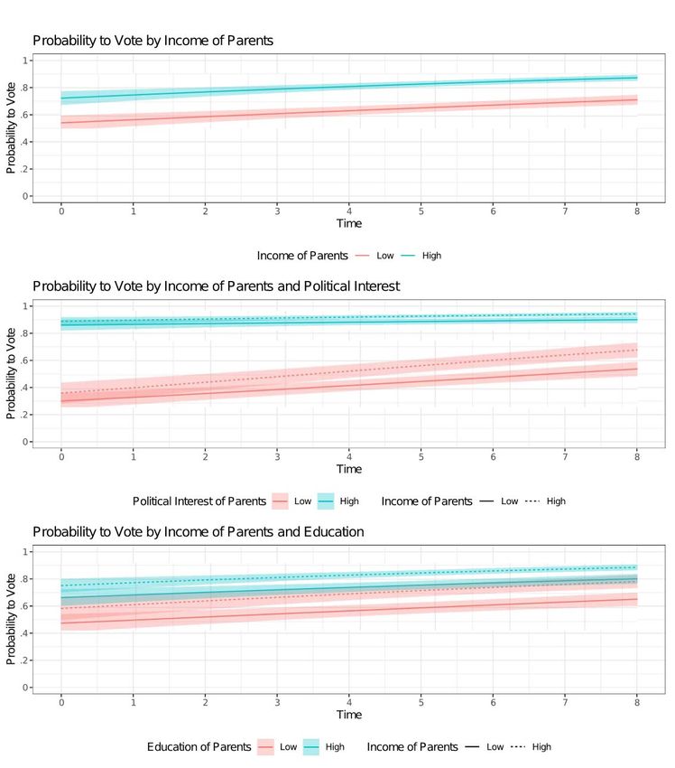
The results are shown as probabilities to vote by age and parental variables. Individual control
variables are held constant at the values for a nonmigrant woman with medium education
(Figure 4). Each panel shows the starting levels of voting propensity at timepoint 0, i.e., the
time when respondents enter the panel between ages 16 and 18. The upper panel shows that
our hypothetical individual from a low/high income family has a 55/73 percent probability to
vote. Hence, there is a gap of almost 20 percentage points depending on whether parents are
in the second or ninth income decile. As indicated by the similar slopes, there is little change
in this gap. After eight years, the difference is still at around 16 percentage points.
Importantly, the effects of parental income might be inflated because of a correlation with the
more directly relevant variables of parental education and political interest. The center panel
16shows that parental political interest plays a much larger role than income. Low parental
interest is linked to a voting probability of only about 35 percent, regardless of whether the
family is poor or rich. If parental political interest is high, the propensity jumps to a whopping
87 percent. However, parental income has an independent influence on the slope at low levels
of parental interest. Hence, high income helps to at least partly compensate for low parental
interest. Still, income is a considerably weaker predictor than interest (which is not entirely
surprising, because it should be further away from participation in the causal chain). Although
the turnout difference between high and low-interest families decreases substantially over
time, it remains at around 35 percentage points (25 percentage points for high income
families). These gaps are substantially higher than the differences between poor and rich
families (13/4 percentage points for families with low/high political interest).
Finally, the bottom panel shows that parental education also has a slightly stronger impact on
voting propensity than parental income. The educational starting gap is roughly 19/16
percentage points for low/high income. At the same time, the difference by income is merely
around 10 percentage points at both levels of parental education. However, another way to
look at the results is that parental income retains a substantial effect on participatory
inequality when education is held constant. Again, this pattern continues over early adulthood.
In all models the differences by parental background are similar for young men (not shown),
although the intercepts are on average higher and the slopes smaller.
We ran additional models for voting intention in the British data (Figure A-3) and voting in
Switzerland (Figure A-4). Overall, the patterns are quite similar to those presented here for
vote intention. Given the above-mentioned overreporting of voting in the SHP, the effects are
less strong. But also here, the parental influence is clearly visible and political interest
emerges as the strongest predictor. Thus, we have to conclude that parental income plays a
significant but comparatively small role in the development of political involvement. Parental
interest in politics is far more important and seems to translate into strong political
participation from an early age.
17Figure 4: Latent growth curve models for probability to vote in the United Kingdom
Note: Plots are based on predictions from latent growth curve models for non-migrant women with medium
education. “Low” and “high” income of parents refers the second and the ninth equivalized household income
deciles. For political interest these values represent either being “not at all interested” (low) or “very interested”
(high) in politics. For parental education “low” indicates having no degree or a degree lower than GCSE and
“high” indicates having achieved A-Levels or higher.
18Conclusions
This article has provided the most comprehensive analysis to date of how income and political
involvement are related in longitudinal data. Our study uses many datasets, specifications, and
operationalizations, which helps us to avoid over-interpreting chance findings and provides a
stronger basis for generalization. Indeed, we found a number of effects for single variables
that might look relevant in isolation. However, our encompassing analysis has mostly
revealed them to be outliers in the broader picture. In sum, we see this article as a step
towards consolidating knowledge on important research questions that so far have received a
rather disparate treatment. While it confirms some previous analyses, it challenges others.
Most clearly, our results confirm Prior’s (2019: 270) verdict that “Income really does not
affect political interest, no matter how we look at it” but generalizes them to a considerably
larger number of countries and, crucially, measures of political involvement. Taken together,
our results and Prior’s (2019) results strongly support the theoretical position that political
involvement is habitual and hardly influenced by short-term income changes. The often-
reported negative correlation between income and voting is most likely spurious.
Regarding RQ2, we could not generalize the argument by Emmenegger et al. (2017) about the
“impressionable years” as a period of heightened responsiveness to socio-economic shocks.
We did not detect a significant interaction between young age and income changes as
predictors of political involvement. A possible reason for the diverging findings is that
Emmenegger et al. (2017) focused on youth unemployment, which might have distinct socio-
emotional repercussions. Our findings are also inconsistent with Ojeda’s (2018) argument that
the importance of personal income increases over the life course. We do acknowledge,
however, that the question of life-course variation deserves treatment in a separate paper in
which finer-grained methods can be explored (such as the difference-in-difference matching
in Emmenegger et al. 2017). It might also be necessary to explicitly model age-specific
experiences, such as economic problems in conjunction with labor-market entry or family
formation.
Importantly, we cannot rule out the possibility that income-related processes within the family
prior to voting age interfere with political socialization. Indeed, our analysis of socialization
trajectories shows that the income gradient in political participation is already large among
first-time voters. Moreover, voters from low-income families do not, on average, catch up. At
least tentatively, we can generalize the important finding by Schlozman et al. (2012) of
inequality at the starting line beyond the US case. That said, we also reaffirm concerns that
their notion of “socio-economic status” is too broad a concept when seeking to understand
income effects (Lahtinen et al. 2019). In fact, differences by parental income are partly
confounded with parental education and politicization (although an independent income effect
remains when controlling for these variables).
Taken together, our findings demonstrate the need for future research to focus on the
influence of socio-economic experiences during childhood and adolescence. Again, our
approach certainly does not exhaust possible and useful research strategies. First and
foremost, an effort comparable to the one in this paper will be necessary to compile panel data
on younger respondents. As shown by Akee et al. (2020), we have to observe respondents as
early as possible to capture all effects of socio-economic variables. As several household
19panels have started to use youth questionnaires and as education panels often include political
variables, this appears increasingly feasible. Moreover, there is a need to develop clearer
theoretical guidelines on the underlying psychological dynamics. For example, socio-
economic problems might hamper political learning in the family because of stressed parents.
But they might also operate through an impact on students’ performance at school and other
indirect mechanisms. Relatedly, researchers will have to develop designs that separate
different aspects of socio-economic family characteristics and possibly study their interaction.
In any case, understanding the socialization processes underlying political inequality should
be a major research goal for political behavior scholars in the coming years.
References
Akee, Randall, William Copeland, John B Holbein, and Emilia Simeonova. 2020. "Human
Capital and Voting Behavior across Generations: Evidence from an Income Intervention."
American Political Science Review 114(2): 609-616.
Aytaç, S Erdem, Eli Gavin Rau, and Susan Stokes. 2020. "Beyond Opportunity Costs:
Campaign Messages, Anger and Turnout among the Unemployed." British Journal of
Political Science 50(4): 1325-1339.
Bell, Andrew, and Kelvyn Jones. 2015. "Explaining fixed effects: Random effects modeling
of time-series cross-sectional and panel data." Political Science Research and Methods 3(1):
133-153.
Brody, Richard A, and Paul M Sniderman. 1977. "From life space to polling place: The
relevance of personal concerns for voting behavior." British Journal of Political Science
7(3): 337-360.
Cesarini, David, Magnus Johannesson, and Sven Oskarsson. 2014. "Pre-birth factors, post-
birth factors, and voting: Evidence from Swedish adoption data." American Political Science
Review 108(1): 71-87.
Dalton, Russell J. 2017. The participation gap: Social status and political inequality. Oxford:
Oxford University Press.
De Boef, Suzanna, and Luke Keele. 2008. "Taking time seriously." American Journal of
Political Science 52(1): 184-200.
Denny, Kevin, and Orla Doyle. 2008. "Political interest, cognitive ability and personality:
Determinants of voter turnout in Britain." British Journal of Political Science 38(2): 291-
310.
Denny, Kevin, and Orla Doyle. 2009. "Does voting history matter? Analysing persistence in
turnout." American Journal of Political Science 53(1): 17-35.
Dinas, Elias. 2013. "Opening “Openness to Change” Political Events and the Increased
Sensitivity of Young Adults." Political Research Quarterly 66(4): 868-882.
Emmenegger, Patrick, Paul Marx, and Dominik Schraff. 2017. "Off to a bad start:
Unemployment and political interest during early adulthood." Journal of Politics 79(1): 315-
328.
Erikson, Robert S. 2015. "Income Inequality and Policy Responsiveness." Annual Review of
Political Science 18: 11-29.
20You can also read