A new look at state-space models for neural data
←
→
Page content transcription
If your browser does not render page correctly, please read the page content below
J Comput Neurosci (2010) 29:107–126
DOI 10.1007/s10827-009-0179-x

A new look at state-space models for neural data
Liam Paninski · Yashar Ahmadian ·
Daniel Gil Ferreira · Shinsuke Koyama ·
Kamiar Rahnama Rad · Michael Vidne ·
Joshua Vogelstein · Wei Wu

Received: 22 December 2008 / Revised: 6 July 2009 / Accepted: 16 July 2009 / Published online: 1 August 2009
© Springer Science + Business Media, LLC 2009

Abstract State space methods have proven indispens-                 setting at all; instead, the key property we are exploiting
able in neural data analysis. However, common meth-                 involves the bandedness of certain matrices. We close
ods for performing inference in state-space models with             by discussing some applications of this more general
non-Gaussian observations rely on certain approxima-                point of view, including Markov chain Monte Carlo
tions which are not always accurate. Here we review                 methods for neural decoding and efficient estimation of
direct optimization methods that avoid these approxi-               spatially-varying firing rates.
mations, but that nonetheless retain the computational
efficiency of the approximate methods. We discuss a                 Keywords Neural coding · State-space models ·
variety of examples, applying these direct optimiza-                Hidden Markov model · Tridiagonal matrix
tion techniques to problems in spike train smoothing,
stimulus decoding, parameter estimation, and inference
of synaptic properties. Along the way, we point out                 1 Introduction; forward-backward methods
connections to some related standard statistical meth-                for inference in state-space models
ods, including spline smoothing and isotonic regression.
Finally, we note that the computational methods re-                 A wide variety of neuroscientific data analysis problems
viewed here do not in fact depend on the state-space                may be attacked fruitfully within the framework of
                                                                    hidden Markov (“state-space”) models. The basic idea
                                                                    is that the underlying system may be described as a
Action Editor: Israel Nelken                                        stochastic dynamical process: a (possibly multidimen-
                                                                    sional) state variable qt evolves through time according
L. Paninski (B) · Y. Ahmadian · D. G. Ferreira ·
K. Rahnama Rad · M. Vidne
                                                                    to some Markovian dynamics p(qt |qt−1 , θ ), as specified
Department of Statistics and Center for Theoretical                 by a few model parameters θ. Now in many situations
Neuroscience, Columbia University,                                  we do not observe the state variable qt directly (this
New York, NY, USA                                                   Markovian variable is “hidden”); instead, our observa-
e-mail: liam@stat.columbia.edu
                                                                    tions yt are a noisy, subsampled version of qt , summa-
URL: http://www.stat.columbia.edu/∼liam
                                                                    rized by an observation distribution p(yt |qt ).
S. Koyama                                                              Methods for performing optimal inference and esti-
Department of Statistics, Carnegie Mellon University,               mation in these hidden Markov models are very well-
Pittsburgh, PA, USA
                                                                    developed in the statistics and engineering literature
J. Vogelstein                                                       (Rabiner 1989; Durbin and Koopman 2001; Doucet
Department of Neuroscience, Johns Hopkins University,               et al. 2001). For example, to compute the conditional
Baltimore, MD, USA                                                  distribution p(qt |Y1:T ) of the state variable qt given
W. Wu
                                                                    all the observed data on the time interval (0, T],
Department of Statistics, Florida State University,                 we need only apply two straightforward recursions: a
Tallahassee, FL, USA                                                forward recursion that computes the conditional dis-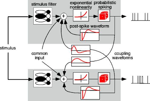
108                                                                                           J Comput Neurosci (2010) 29:107–126

tribution of qt given only the observed data up to                    tions, where estimates must be updated in real time as
time t,                                                               new information is observed. For example, state-space
                                                                     techniques achieve state-of-the-art performance decod-
p(qt |Y1:t ) ∝ p(yt |qt ) p(qt |qt−1 ) p(qt−1 |Y1:t−1 )dqt−1 ,        ing multineuronal spike train data from motor cortex
                                                                      (Wu et al. 2006; Truccolo et al. 2005; Wu et al. 2009)
            for t = 1, 2, . . . , T                            (1)    and parietal cortex (Yu et al. 2006; Kemere et al. 2008),
                                                                      and these methods therefore hold great promise for the
and then a backward recursion that computes the de-
                                                                      design of motor neuroprosthetic devices (Donoghue
sired distribution p(qt |Y1:T ),
                                                                      2002). In this setting, the hidden variable qt corresponds

                              p(qt+1 |Y1:T ) p(qt+1 |qt )             to the desired position of the subject’s hand, or a cursor
p(qt |Y1:T ) = p(qt |Y1:t )                                dqt+1 ,   on a computer screen, at time t; yt is the vector of
                               p(qt+1 |qt ) p(qt |Y1:t )dqt
                                                                      observed spikes at time t, binned at some predeter-
            for t = T −1, T −2, . . . , 1, 0.                  (2)    mined temporal resolution; the conditional probability
                                                                      p(yt |qt ) is given by an “encoding” model that describes
Each of these recursions may be derived easily from                   how the position information qt is represented in the
the Markov structure of the state-space model. In                     spike trains yt ; and p(qt |Y1:t+s ) is the desired fixed-
the classical settings, where the state variable q is dis-            lag decoding distribution, summarizing our knowledge
crete (Rabiner 1989; Gat et al. 1997; Hawkes 2004;                    about the current position qt given all of the observed
Jones et al. 2007; Kemere et al. 2008; Herbst et al. 2008;            spike train data Y from time 1 up to t + s, where s
Escola and Paninski 2009), or the dynamics p(qt |qt−1 )               is a short allowed time lag (on the order of 100 ms
and observations p(yt |qt ) are linear and Gaussian, these            or so in motor prosthetic applications). In this setting,
recursions may be computed exactly and efficiently:                   the conditional expectation E(qt |Y1:t+s ) is typically used
note that a full forward-backward sweep requires com-                 as the optimal (minimum mean-square) estimator for
putation time which scales just linearly in the data                  qt , while the posterior covariance Cov(qt |Y1:t+s ) quan-
length T, and is therefore quite tractable even for                   tifies our uncertainty about the position qt , given the
large T. In the linear-Gaussian case, this forward-                   observed data; both of these quantities are computed
backward recursion is known as the Kalman filter-                     most efficiently using the forward-backward recur-
smoother (Roweis and Ghahramani 1999; Durbin and                      sions (1–2). These forward-backward methods can also
Koopman 2001; Penny et al. 2005; Shumway and Stoffer                  easily incorporate target or endpoint goal information
2006).                                                                in these online decoding tasks (Srinivasan et al. 2006;
    Unfortunately, the integrals in Eqs. (1) and (2) are              Yu et al. 2007; Kulkarni and Paninski 2008; Wu et al.
not analytically tractable in general; in particular, for             2009).
neural applications we are interested in cases where the                  State-space models have also been applied success-
observations yt are point processes (e.g., spike trains, or           fully to track nonstationary neuron tuning properties
behavioral event times), and in this case the recursions              (Brown et al. 2001; Frank et al. 2002; Eden et al. 2004;
must be solved approximately. One straightforward                     Czanner et al. 2008; Rahnama et al. 2009). In this case,
idea is to approximate the conditional distributions                  the hidden state variable qt represents a parameter vec-
appearing in (1) and (2) as Gaussian; since we can com-               tor which determines the neuron’s stimulus-response
pute Gaussian integrals analytically (as in the Kalman                function. Lewi et al. (2009) discusses an application
filter), this simple approximation provides a computa-                of these recursive methods to perform optimal online
tionally tractable, natural extension of the Kalman filter            experimental design — i.e., to choose the stimulus at
to non-Gaussian observations. Many versions of this                   time t which will give us as much information as possi-
recursive Gaussian approximation idea (with varying                   ble about the observed neuron’s response properties,
degrees of accuracy versus computational expediency)                  given all the observed stimulus-response data from
have been introduced in the statistics and neuroscience               time 1 to t.
literature (Fahrmeir and Kaufmann 1991; Fahrmeir and                      A number of offline applications have appeared as
Tutz 1994; Bell 1994; Kitagawa and Gersch 1996; West                  well: state-space methods have been applied to per-
and Harrison 1997; Julier and Uhlmann 1997; Brown                     form optimal decoding of rat position given multiple
et al. 1998; Smith and Brown 2003; Ypma and Heskes                    hippocampal spike trains (Brown et al. 1998; Zhang
2003; Eden et al. 2004; Yu et al. 2006).                              et al. 1998; Eden et al. 2004), and to model behavioral
    These methods have proven extremely useful in a                   learning experiments (Smith and Brown 2003; Smith
wide variety of neural applications. Recursive estima-                et al. 2004, 2005; Suzuki and Brown 2005); in the
tion methods are especially critical in online applica-               latter case, qt represents the subject’s certainty about
J Comput Neurosci (2010) 29:107–126 109
the behavioral task, which is not directly observable model, (Q, Y) forms a jointly Gaussian random vector,
and which changes systematically over the course of and therefore p(Q|Y) is itself Gaussian. Since the mean
the experiment. In addition, we should note that the and mode of a Gaussian distribution coincide, this im-
forward-backward idea is of fundamental importance plies that E(Q|Y) is equal to the maximum a poste-
in the setting of sequential Monte Carlo (“particle- riori (MAP) solution, the maximizer of the posterior
filtering”) methods (Doucet et al. 2001; Brockwell et al. p(Q|Y). If we write out the linear-Gaussian Kalman
2004; Kelly and Lee 2004; Godsill et al. 2004; Shoham model more explicitly,
et al. 2005; Ergun et al. 2007; Vogelstein et al. 2009;
qt = Aqt−1 + t , t ∼ N (0, Cq ); q1 ∼ N (μ1 , C1 )
Huys and Paninski 2009), though we will not focus on
these applications here. yt = Bqt + ηt , ηt ∼ N (0, C y )
However, the forward-backward approach is not al-
(where N (0, C) denotes the Gaussian density with
ways directly applicable. For example, in many cases
mean 0 and covariance C), we can gain some insight
the dynamics p(qt |qt−1 ) or observation density p(yt |qt )
into the the analytical form of this maximizer:
may be non-smooth (e.g., the state variable q may be
constrained to be nonnegative, leading to a discontinu- E(Q|Y) = arg max p(Q|Y)
Q
ity in log p(qt |qt−1 ) at qt = 0). In these cases the forward
distribution p(qt |Y1:t ) may be highly non-Gaussian, and = arg max log p(Q, Y)
Q
the basic forward-backward Gaussian approximation
methods described above may break down.1 In this
T
paper, we will review more general direct optimiza- = arg max log p(q1 ) + log p(qt |qt−1 )
Q
t=2
tion methods for performing inference in state-space
models. We discuss this approach in Section 2 below.
T
This direct optimization approach also leads to more + log p(yt |qt )
t=1
efficient methods for estimating the model parameters
θ (Section 3). Finally, the state-space model turns out 1
= arg max − (q1 −μ1 )T C1−1 (q1 −μ1 )
to be a special case of a richer, more general framework Q 2
involving banded matrix computations, as we discuss at
T
more length in Section 4. + (qt − Aqt−1 )T Cq−1 (qt − Aqt−1 )
t=2
2 A direct optimization approach for computing
T
+ (yt − Bqt )T C−1
y (yt − Bqt ) .
the maximum a posteriori path in state-space models t=1
2.1 A direct optimization interpretation (3)
of the classical Kalman filter The right-hand-side here is a simple quadratic func-
tion of Q (as expected, since p(Q|Y) is Gaussian, i.e.,
We begin by taking another look at the classical log p(Q|Y) is quadratic), and therefore E(Q|Y) may
Kalman filter-smoother (Durbin and Koopman 2001; be computed by solving an unconstrained quadratic
Wu et al. 2006; Shumway and Stoffer 2006). The pri- program in Q; we thus obtain
mary goal of the smoother is to compute the conditional
1 T
expectation E(Q|Y) of the hidden state path Q given Q̂ = arg max log p(Q|Y) = arg max Q HQ + ∇T Q
the observations Y. (Throughout this paper, we will use
Q Q 2
Q and Y to denote the full collection of the hidden = −H −1 ∇,
state variables {qt } and observations {yt }, respectively.)
where we have abbreviated the Hessian and gradient of
Due to the linear-Gaussian structure of the Kalman
log p(Q|Y):
1 Itis worth noting that other more sophisticated methods such ∇ = ∇ Q log p(Q|Y) Q=0
as expectation propagation (Minka 2001; Ypma and Heskes
2003; Yu et al. 2006, 2007; Koyama and Paninski 2009) may be
better-equipped to handle these strongly non-Gaussian observa- H = ∇∇ Q log p(Q|Y) Q=0
.
tion densities p(yt |qt ) (and are, in turn, closely related to the
optimization-based methods that are the focus of this paper);
however, due to space constraints, we will not discuss these The next key point to note is that the Hessian matrix
methods at length here. H is block-tridiagonal, since log p(Q|Y) is a sum of sim-110 J Comput Neurosci (2010) 29:107–126
ple one-point potentials (log p(qt ) and log p(yt |qt )) and of our Gaussian vector Q given Y, Cov(qt |Y) is given
nearest-neighbor two-point potentials (log p(qt , qt−1 )). by the (t, t)-th block of H −1 , and it is well-known that
More explicitly, we may write the diagonal and off-diagonal blocks of the inverse of
a block-tridiagonal matrix can be computed in O(T)
⎛ ⎞
T
D1 R1,2 0 ··· 0 time; again, the full inverse H −1 (which requires O(T 2 )
⎜ ⎟ .. time in the block-tridiagonal case) is not required
⎜ R1,2 D2 R2,3
T
0 ⎟ .
⎜ ⎟ (Rybicki and Hummer 1991; Rybicki and Press 1995;
⎜ . .. ⎟
⎜ 0 R2,3 D3 R3,4 ⎟
H=⎜ ⎟ (4) Asif and Moura 2005).
⎜ . . .. .. ⎟
⎜ .. .. . . 0 ⎟
⎜ ⎟
⎝ D N−1 R N−1,N ⎠
T
2.2 Extending the direct optimization method
0 ··· 0 R N−1,N D N
to non-Gaussian models
where
From here it is straightforward to extend this approach
∂ 2
∂ 2 to directly compute Q̂ M AP in non-Gaussian models of
Di = log p(yi |qi ) + 2 log p(qi |qi−1 ) interest in neuroscience. In this paper we will focus
∂qi2 ∂qi
on the case that log p(qt+1 |qt ) is a concave function of
∂2 Q; in addition, we will assume that the initial density
+ log p(qi+1 |qi ), (5)
∂qi2 log p(q0 ) is concave and also that the observation den-
sity log p(yt |qt ) is concave in qt . Then it is easy to see
and that the log-posterior
∂2 log p(Q|Y) = log p(q0 ) + log p(yt |qt )
Ri,i+1 = log p(qi+1 |qi ) (6)
∂qi ∂qi+1 t
+ log p(qt+1 |qt ) + const.
for 1 < i < N. These quantities may be computed as t
simple functions of the Kalman model parameters; for
example, Ri,i+1 = Cq−1 A. is concave in Q, and therefore computing the MAP
This block-tridiagonal form of H implies that the path Q̂ is a concave problem. Further, if log p(q0 ),
linear equation Q̂ = H −1 ∇ may be solved in O(T) time log p(yt |qt ), and log p(qt+1 |qt ) are all smooth functions
(e.g., by block-Gaussian elimination (Press et al. 1992); of Q, then we may apply standard approaches such as
note that we never need to compute H −1 explicitly). Newton’s algorithm to solve this concave optimization.
Thus this matrix formulation of the Kalman smoother is To apply Newton’s method here, we simply itera-
equivalent both mathematically and in terms of compu- tively solve the linear equation2
tational complexity to the forward-backward method.
In fact, the matrix formulation is often easier to im- Q̂(i+1) = Q̂(i) − H −1 ∇,
plement; for example, if H is sparse and banded, the
standard Matlab backslash command Q̂ = H\∇ calls where we have again abbreviated the Hessian and gra-
the O(T) algorithm automatically—Kalman smoothing dient of the objective function log p(Q|Y):
in just one line of code.
We should also note that a second key application ∇ = ∇ Q log p(Q|Y) Q= Q̂(i)
of the Kalman filter is to compute the posterior state
covariance Cov(qt |Y) and also the nearest-neighbor
second moments E(qt qt+1 T
|Y); the posterior covariance H = ∇∇ Q log p(Q|Y) Q= Q̂(i)
.
is required for computing confidence intervals around
the smoothed estimates E(qt |Y), while the second mo- Clearly, the only difference between the general non-
ments E(qt qt+1T
|Y) are necessary to compute the suf- Gaussian case here and the special Kalman case
ficient statistics in the expectation-maximization (EM)
algorithm for estimating the Kalman model parameters
2 In practice, the simple Newton iteration does not always in-
(see, e.g., Shumway and Stoffer 2006 for details). These
crease the objective log p(Q|Y); we have found the standard
quantities may easily be computed in O(T) time in remedy for this instability (perform a simple backtracking line-
the matrix formulation. For example, since the matrix search along the Newton direction Q̂(i) − δ (i) H −1 ∇ to determine
H represents the inverse posterior covariance matrix a suitable stepsize δ (i) ≤ 1) to be quite effective here.J Comput Neurosci (2010) 29:107–126 111
described above is that the Hessian H and gradient major question now is how accurately this inferred
∇ must be recomputed at each iteration Q̂(i) ; in the functional connectivity actually reflects the true under-
Kalman case, again, log p(Q|Y) is a quadratic function, lying anatomical connectivity in the circuit.
and therefore the Hessian H is constant, and one it- Fewer models, however, have attempted to include
eration of Newton’s method suffices to compute the the effects of the population of neurons which are
optimizer Q̂. not directly observed during the experiment (Nykamp
In practice, this Newton algorithm converges within 2005, 2007; Kulkarni and Paninski 2007). Since we can
a few iterations for all of the applications discussed directly record from only a small fraction of neurons in
here. Thus we may compute the MAP path exactly any physiological preparation, such unmeasured neu-
using this direct method, in time comparable to that rons might have a large collective impact on the dy-
required to obtain the approximate MAP path com- namics and coding properties of the observed neural
puted by the recursive approximate smoothing algo- population, and may bias the inferred functional con-
rithm discussed in Section 1. This close connection nectivity away from the true anatomical connectivity,
between the Kalman filter and the Newton-based com- complicating the interpretation of these multineuronal
putation of the MAP path in more general state-space analyses. For example, while Pillow et al. (2008) found
models is well-known in the statistics and applied math that neighboring parasol retinal ganglion cells (RGCs)
literature (though apparently less so in the neurosci- in the macaque are functionally coupled — indeed,
ence literature). See Fahrmeir and Kaufmann (1991), incorporating this functional connectivity in an opti-
Fahrmeir and Tutz (1994), Bell (1994), Davis and mal Bayesian decoder significantly amplifies the in-
Rodriguez-Yam (2005), Jungbacker and Koopman formation we can extract about the visual stimulus
(2007) for further discussion from a statistical point from the observed spiking activity of large ensembles
of view, and Koyama and Paninski (2009) for ap- of RGCs — Khuc-Trong and Rieke (2008) recently
plications to the integrate-and-fire model for spiking demonstrated, via simultaneous pairwise intracellular
data. In addition, Yu et al. (2007) previously applied recordings, that RGCs receive a significant amount of
a related direct optimization approach in the con- strongly correlated common input, with weak direct
text of neural decoding (though note that the conju- anatomical coupling between RGCs. Thus the strong
gate gradients approach utilized there requires O(T 3 ) functional connectivity observed in this circuit is in fact
time if the banded structure of the Hessian is not largely driven by common input, not direct anatomical
exploited). connectivity.
Therefore it is natural to ask if it is possible to
correctly infer the degree of common input versus
2.3 Example: inferring common input effects direct coupling in partially-observed neuronal circuits,
in multineuronal spike train recordings given only multineuronal spike train data (i.e., we do
not want to rely on multiple simultaneous intracellular
Recent developments in multi-electrode recording recordings, which are orders of magnitude more dif-
technology (Nicolelis et al. 2003; Litke et al. 2004) ficult to obtain than extracellular recordings). To this
and fluorescence microscopy (Cossart et al. 2003; Ohki end, Kulkarni and Paninski (2007) introduced a state-
et al. 2005; Nikolenko et al. 2008) enable the simul- space model in which the firing rates depend not only
taneous measurement of the spiking activity of many on the stimulus history and the spiking history of the
neurons. Analysis of such multineuronal data is one observed neurons but also on common input effects
of the key challenges in computational neuroscience (Fig. 1). In this model, the conditional firing intensity,
today (Brown et al. 2004), and a variety of mod- λi (t), of the i-th observed neuron is:
els for these data have been introduced (Chornoboy ⎛
et al. 1988; Utikal 1997; Martignon et al. 2000; Iyengar
⎝
λi (t) = exp ki · x(t) + hi · yi (t) + lij · y j(t)
2001; Schnitzer and Meister 2003; Paninski et al. 2004;
i= j
Truccolo et al. 2005; Nykamp 2005; Schneidman et al.
⎞
2006; Shlens et al. 2006; Pillow et al. 2008; Shlens
et al. 2009). Most of these models include stimulus- +μi + qi (t)⎠ , (7)
dependence terms and “direct coupling” terms repre-
senting the influence that the activity of an observed
cell might have on the other recorded neurons. These where x is the spatiotemporal visual stimulus, yi is cell
coupling terms are often interpreted in terms of “func- i’s own spike-train history, μi is the cell’s baseline log-
tional connectivity” between the observed neurons; the firing rate, y j are the spike-train histories of other cells112 J Comput Neurosci (2010) 29:107–126
preliminary experiments is indistinguishable from those
described in Pillow et al. (2008), where a model with
strong direct-coupling terms and no common-input ef-
fects was used.
Given the estimated model parameters θ , we used
the direct optimization method to estimate the sub-
threshold common input effects q(t), on a single-trial
basis (Fig. 2). The observation likelihood p(yt |qt ) here
was given by the standard point-process likelihood
(Snyder and Miller 1991):
log p(Y|Q) = yit log λi (t) − λi (t)dt, (8)
it
Fig. 1 Schematic illustration of the common-input model de-
scribed by Eq. (7); adapted from Kulkarni and Paninski (2007)
where yit denotes the number of spikes observed in
time bin t from neuron i; dt denotes the temporal bin-
width. We see in Fig. 2 that the inferred common input
effect is strong relative to the direct coupling effects, in
at time t, ki is the cell’s spatiotemporal stimulus filter,
agreement with the intracellular recordings described
hi is the post-spike temporal filter accounting for past
in Khuc-Trong and Rieke (2008). We are currently
spike dependencies within cell i, and lij are direct cou-
working to quantify these common input effects qi (t)
pling temporal filters, which capture the dependence
inferred from the full observed RGC population, rather
of cell i’s activity on the recent spiking of other cells
than just the pairwise analysis shown here, in order
j. The term qi (t), the hidden common input at time t,
to investigate the relevance of this strong common
is modeled as a Gauss-Markov autoregressive process,
input effect on the coding and correlation properties
with some correlation between different cells i which
of the full network of parasol cells. See also Wu et al.
we must infer from the data. In addition, we enforce a
(2009) for applications of similar common-input state-
nonzero delay in the direct coupling terms, so that the
space models to improve decoding of population neural
effects of a spike in one neuron on other neurons are
activity in motor cortex.
temporally strictly causal.
In statistical language, this common-input model is
a multivariate version of a Cox process, also known
as a doubly-stochastic point process (Cox 1955; Snyder 2.4 Constrained optimization problems
and Miller 1991; Moeller et al. 1998); the state-space may be handled easily via the log-barrier
models applied in Smith and Brown (2003), Truccolo method
et al. (2005), Czanner et al. (2008) are mathematically
very similar. See also Yu et al. (2006) for discussion of So far we have assumed that the MAP path may be
a related model in the context of motor planning and computed via an unconstrained smooth optimization.
intention. In many examples of interest we have to deal with con-
As an example of the direct optimization methods strained optimization problems instead. In particular,
developed in the preceding subsection, we reanalyzed nonnegativity constraints arise frequently on physical
the data from Pillow et al. (2008) with this common grounds; as emphasized in the introduction, forward-
input model (Vidne et al. 2009). We estimated the backward methods based on Gaussian approximations
model parameters θ = (ki , hi , lij, μi ) from the spiking for the forward distribution p(qt |Y0:t ) typically do not
data by maximum marginal likelihood, as described accurately incorporate these constraints. To handle
in Koyama and Paninski (2009) (see also Section 3 these constrained problems while exploiting the fast
below, for a brief summary); the correlation time of Q tridiagonal techniques discussed above, we can employ
was set to ∼ 5 ms, to be consistent with the results of standard interior-point (aka “barrier”) methods (Boyd
Khuc-Trong and Rieke (2008). We found that this and Vandenberghe 2004; Koyama and Paninski 2009).
common-input model explained the observed cross- The idea is to replace the constrained concave problem
correlations quite well (data not shown), and the in-
ferred direct-coupling weights were set to be relatively Q̂ M AP = arg max log p(Q|Y)
small (Fig. 2); in fact, the quality of the fits in our Q:qt ≥0J Comput Neurosci (2010) 29:107–126 113
common input
1
0
–1
–2
direct coupling input
1
0
–1
–2
stimulus input
2
0
–2
refractory input
0
–1
–2
spikes
100 200 300 400 500 600 700 800 900 1000
ms
Fig. 2 Single-trial inference of the relative contribution of com- (The first two panels are plotted on the same scale to facilitate
mon, stimulus, direct coupling, and self inputs in a pair of retinal comparison of the magnitudes of these effects.) Blue trace indi-
ganglion ON cells (Vidne et al. 2009); data from (Pillow et al. cates cell 1; green indicates cell 2. 3rd panel: The stimulus input,
2008). Top panel: Inferred linear common input, Q̂: red trace k · x. 4th panel: Refractory input, hi · yi . Note that this term is
shows a sample from the posterior distribution p(Q|Y), black strong but quite short-lived following each spike. All units are
trace shows the conditional expectation E(Q|Y), and shaded in log-firing rate, as in Eq. (7). Bottom: Observed paired spike
region indicates ±1 posterior standard deviation about E(Q|Y), trains Y on this single trial. Note the large magnitude of the
computed from the diagonal of the inverse log-posterior Hessian estimated common input term q̂(t), relative to the direct coupling
H. 2nd panel: Direct coupling input from the other cell, l j · y j . contribution l j · y j
with a sequence of unconstrained concave problems Newton iteration to obtain Q̂ , for any , and then
sequentially decrease (in an outer loop) to obtain
Q̂ = arg max log p(Q|Y) + log qt ; Q̂. Note that the approximation arg max Q p(Q|Y) ≈
Q E(Q|Y) will typically not hold in this constrained case,
t
since the mean of a truncated Gaussian distribution will
clearly, Q̂ satisfies the nonnegativity constraint, since typically not coincide with the mode (unless the mode
log u → −∞ as u → 0. (We have specialized to the is sufficiently far from the nonnegativity constraint).
nonnegative case for concreteness, but the idea may We give a few applications of this barrier approach
be generalized easily to any convex constraint set; see below. See also Koyama and Paninski (2009) for a
Boyd and Vandenberghe 2004 for details.) Further- detailed discussion of an application to the integrate-
more, it is easy to show that if Q̂ M AP is unique, then and-fire model, and Vogelstein et al. (2008) for appli-
Q̂ converges to Q̂ M AP as → 0. cations to the problem of efficiently deconvolving slow,
Now the key point is that the noisy calcium fluorescence traces to obtain nonnegative
Hessian of the
objective function log p(Q|Y) + t log qt retains the estimates of spiking times. In addition, see Cunningham
block-tridiagonal properties of the original objective et al. (2008) for an application of the log-barrier method
log p(Q|Y), since the barrier term contributes a simple to infer firing rates given point process observations in
diagonal term to H. Therefore we may use the O(T) a closely-related Gaussian process model (Rasmussen114 J Comput Neurosci (2010) 29:107–126
and Williams 2006); these authors considered a slightly impose hard Lipschitz constraints on Q, instead of the
more general class of covariance functions on the latent soft quadratic penalties imposed in the Gaussian state-
stochastic process qt , but the computation time of the space setting: we assume
resulting method scales superlinearly3 with T.
|qt − qs | < K|t − s|
2.4.1 Example: point process smoothing
under Lipschitz or monotonicity for all (s, t), for some finite constant K. (If qt is a
constraints on the intensity function differentiable function of t, this is equivalent to the
assumption that the maximum absolute value of the
A standard problem in neural data analysis is to derivative of Q is bounded by K.) The space of all such
smooth point process observations; that is, to estimate Lipschitz Q is convex, and so optimizing the concave
the underlying firing rate λ(t) given single or multi- loglikelihood function under this convex constraint re-
ple observations of a spike train (Kass et al. 2003). mains tractable. Coleman and Sarma (2007) presented
One simple approach to this problem is to model a powerful method for solving this optimization prob-
the firing rate as λ(t) = f (qt ), where f (.) is a convex, lem (their solution involved a dual formulation of the
log-concave, monotonically increasing nonlinearity problem and an application of specialized fast min-
(Paninski 2004) and qt is an unobserved function of cut optimization methods). In this one-dimensional
time we would like to estimate from data. Of course, temporal smoothing case, we may solve this problem
if qt is an arbitrary function, we need to contend with in a somewhat simpler way, without any loss of effi-
overfitting effects; the “maximum likelihood” Q̂ here ciency, using the tridiagonal log-barrier methods de-
would simply set f (qt ) to zero when no spikes are scribed above. We just need to rewrite the constrained
observed (by making −qt very large) and f (qt ) to be problem
very large when spikes are observed (by making qt very
large). max Q log p(Q|Y) s.t. |qt − qs | < K|t − s| ∀s, t
A simple way to counteract this overfitting effect is
to include a penalizing prior; for example, if we model as the unconstrained problem
qt as a linear-Gaussian autoregressive process
qt − qt+dt
max Q log p(Q|Y) + b ,
qt+dt = qt + t , t ∼ N (0, σ 2 dt), t
dt
with dt some arbitrarily small constant and the hard
then computing Q̂ M AP leads to a tridiagonal optimiza-
barrier function b (.) defined as
tion, as discussed above. (The resulting model, again,
is mathematically equivalent to those applied in Smith
0 |u| < K
and Brown 2003, Truccolo et al. 2005, Kulkarni and b (u) =
Paninski 2007, Czanner et al. 2008, Vidne et al. 2009.) −∞ otherwise.
Here 1/σ 2 acts as a regularization parameter: if σ 2 is
small, the inferred Q̂ M AP will be very smooth (since The resulting concave objective function is non-
large fluctuations are penalized by the Gaussian autore- smooth, but may be optimized stably, again, via the
gressive prior), whereas if σ 2 is large, then the prior log-barrier method, with efficient tridiagonal Newton
term will be weak and Q̂ M AP will fit the observed data updates. (In this case, the Hessian of the first term
more closely. log p(Q|Y) with respect to Q is diagonal and the
A different method for regularizing Q was intro- Hessian of the penalty term involving the barrier func-
duced by Coleman and Sarma (2007). The idea is to tion is tridiagonal, since b (.) contributes a two-point
potential here.) We recover the standard state-space
approach if we replace the hard-threshold penalty func-
tion b (.) with a quadratic function; conversely, we may
3 More precisely, Cunningham et al. (2008) introduce a clever obtain sharper estimates of sudden changes in qt if we
iterative conjugate-gradient (CG) method to compute the MAP use a concave penalty b (.) which grows less steeply than
path in their model; this method requires O(T log T) time per a quadratic function (so as to not penalize large changes
CG step, with the number of CG steps increasing as a function of
the number of observed spikes. (Note, in comparison, that the
in qt as strongly), as discussed by Gao et al. (2002).
computation times of the state-space methods reviewed in the Finally, it is interesting to note that we may also easily
current work are insensitive to the number of observed spikes.) enforce monotonicity constraints on qt , by choosing theJ Comput Neurosci (2010) 29:107–126 115
penalty function b (u) to apply a barrier at u = 0; this is given by the convolution gtI = NtI ∗ exp(−t/τ I )), the
is a form of isotonic regression (Silvapulle and Sen log-posterior may be written as
2004), and is useful in cases where we believe that
a cell’s firing rate should be monotonically increasing log p(Q|Y) = log p(Y|Q) + log p(NtI , NtE ) + const.
or decreasing throughout the course of a behavioral
trial, or as a function of the magnitude of an applied
T
stimulus. = log p(Y|Q) + log p(NtE )
t=1
T
2.4.2 Example: inferring presynaptic inputs + log p(NtI ) + const., NtE , NtI ≥ 0;
given postsynaptic voltage recordings t=1
To further illustrate the flexibility of this method, in the case of white Gaussian current noise t with
let’s look at a multidimensional example. Consider the variance σ 2 dt, for example,4 we have
problem of identifying the synaptic inputs a neuron
is receiving: given voltage recordings at a postsynap-
1
T
tic site, is it possible to recover the time course of log p(Y|Q) = − Vt+dt − Vt +dt g L (V L −Vt )
2
2σ dt t=2
the presynaptic conductance inputs? This question has
received a great deal of experimental and analytical
2
attention (Borg-Graham et al. 1996; Peña and Konishi +gtI (V I −Vt )+gtE (V E −Vt ) +const.;
2000; Wehr and Zador 2003; Priebe and Ferster 2005;
Murphy and Rieke 2006; Huys et al. 2006; Wang et al.
this is a quadratic function of Q.
2007; Xie et al. 2007; Paninski 2009), due to the impor-
Now applying the O(T) log-barrier method is
tance of understanding the dynamic balance between
straightforward; the Hessian of the log-posterior
excitation and inhibition underlying sensory informa-
log p(Q|Y) in this case is block-tridiagonal, with
tion processing.
blocks of size two (since our state variable qt is
We may begin by writing down a simple state-space
two-dimensional). The observation term log p(Y|Q)
model for the evolution of the postsynaptic voltage and
contributes a block-diagonal term to the Hessian; in
conductance:
particular, each observation yt contributes a rank-1
matrix of size 2 × 2 to the t-th diagonal block of H. (The
Vt+dt = Vt + dt g L (V L − Vt ) + gtE (V E − Vt ) low-rank nature of this observation matrix reflects the
fact that we are attempting to extract two variables—
+gtI (V I − Vt ) + t the excitatory and inhibitory conductances at each time
step—given just a single voltage observation per time
gtE
E
gt+dt = gtE − dt + NtE step.)
τE Some simulated results are shown in Fig. 3. We
gtI generated Poisson spike trains from both inhibitory and
I
gt+dt = gtI − dt + NtI . (9) excitatory presynaptic neurons, then formed the postsy-
τI
naptic current signal It by contaminating the summed
synaptic and leak currents with white Gaussian noise as
Here gtE denotes the excitatory presynaptic conduc- in Eq. (9), and then used the O(T) log-barrier method
tance at time t, and gtI the inhibitory conductance; to simultaneously infer the presynaptic conductances
V L , V E , and V I denote the leak, excitatory, and
inhibitory reversal potentials, respectively. Finally, t
denotes an unobserved i.i.d. current noise with a log-
concave density, and NtE and NtI denote the presynaptic 4 The approach here can be easily generalized to the case that
excitatory and inhibitory inputs (which must be non-
the input noise has a nonzero correlation timescale. For exam-
negative on physical grounds); we assume these inputs ple, if the noise can be modeled as an autoregressive process
also have a log-concave density. of order p instead of the white noise process described here,
Assume Vt is observed noiselessly for simplicity. then we simply include the unobserved p-dimensional Markov
noise process in our state variable (i.e., our Markov state vari-
Then let our observed variable yt = Vt+dt − Vt and our able qt will now have dimension p + 2 instead of 2), and then
state variable qt = (gtE gtI )T . Now, since gtI and gtE apply the O(T) log-barrier method to this augmented state
are linear functions of NtI and NtE (for example, gtI space.116 J Comput Neurosci (2010) 29:107–126
3
2
true g
1
0
0.1 0.2 0.3 0.4 0.5 0.6 0.7 0.8 0.9 1
100
50
I(t)
0
–50
0.1 0.2 0.3 0.4 0.5 0.6 0.7 0.8 0.9 1
2.5
2
estimated g
1.5
1
0.5
0.1 0.2 0.3 0.4 0.5 0.6 0.7 0.8 0.9 1
time (sec)
Fig. 3 Inferring presynaptic inputs given simulated postsynaptic shrinkage is more evident in the inferred inhibitory conductance,
voltage recordings. Top: true simulated conductance input (green due to the smaller driving force (the holding potential in this
indicates inhibitory conductance; blue excitatory). Middle: ob- experiment was −62 mV, which is quite close to the inhibitory
served noisy current trace from which we will attempt to infer reversal potential; as a result, the likelihood term is much weaker
the input conductance. Bottom: Conductance inferred by nonneg- for the inhibitory conductance than for the excitatory term).
ative MAP technique. Note that inferred conductance is shrunk Inference here required about one second on a laptop computer
in magnitude compared to true conductance, due to the effects per second of data (i.e., real time), at a sampling rate of 1 KHz
of the prior p(NtE ) and p(NtI ), both of which peak at zero here;
from the observed current It . The current was recorded 3 Parameter estimation
at 1 KHz (1 ms bins), and we reconstructed the presy-
naptic activity at the same time resolution. We see that In the previous sections we have discussed the inference
the estimated Q̂ here does a good job extracting both of the hidden state path Q in the case that the system
excitatory and inhibitory synaptic activity given a single parameters are known. However, in most applications,
trace of observed somatic current; there is no need we need to estimate the system parameters as well.
to average over multiple trials. It is worth emphasiz- As discussed in Kass et al. (2005), standard modern
ing that we are inferring two presynaptic signals here methods for parameter estimation are based on the
given just one observed postsynaptic current signal, likelihood p(Y|θ) of the observed data Y given the
with limited “overfitting” artifacts; this is made pos- parameters θ . In the state-space setting, we need to
sible by the sparse, nonnegatively constrained nature compute the marginal likelihood by integrating out the
of the inferred presynaptic signals. For simplicity, we hidden state path Q:5
assumed that the membrane leak, noise variance, and
synaptic time constants τ E and τ I were known here; we p(Y|θ) = p(Q, Y|θ)dQ = p(Y|Q, θ ) p(Q|θ)dQ. (10)
used exponential (sparsening) priors p(NtE ) and p(NtI ),
but the results are relatively robust to the details of
these priors (data not shown). See Huys et al. (2006), 5 Insome cases, Q may be observed directly on some subset of
Huys and Paninski (2009), Paninski (2009) for further training data. If this is the case (i.e., direct observations of qt are
available together with the observed data Y), then the estimation
details and extensions, including methods for inferring
problem simplifies drastically, since we can often fit the models
the membrane parameters directly from the observed p(yt |qt , θ) and p(qt |qt−1 , θ) directly without making use of the
data. more involved latent-variable methods discussed in this section.J Comput Neurosci (2010) 29:107–126 117
This marginal likelihood is a unimodal function of and Raftery 1995; Davis and Rodriguez-Yam 2005; Yu
the parameters θ in many important cases (Paninski et al. 2007) for the marginal likelihood,
2005), making maximum likelihood estimation feasi-
ble in principle. However, this high-dimensional inte- log p(Y|θ) ≈ log p(Y| Q̂θ , θ ) + log p( Q̂θ |θ)
gral can not be computed exactly in general, and so 1
many approximate techniques have been developed, − log | − Hθ | + const. (12)
2
including Monte Carlo methods (Robert and Casella
2005; Davis and Rodriguez-Yam 2005; Jungbacker and Clearly the first two terms here can be computed
Koopman 2007; Ahmadian et al. 2009a) and expecta- in O(T), since we have already demonstrated that
tion propagation (Minka 2001; Ypma and Heskes 2003; we can obtain Q̂θ in O(T) time, and evaluating
Yu et al. 2006; Koyama and Paninski 2009). log p(Y|Q, θ ) + log p(Q|θ) at Q = Q̂θ is relatively
In the neural applications reviewed in Section 1, the easy. We may also compute log | − Hθ | stably and in
most common method for maximizing the loglikelihood O(T) time, via the Cholesky decomposition for banded
is the approximate Expectation-Maximization (EM) matrices (Davis and Rodriguez-Yam 2005; Koyama
algorithm introduced in Smith and Brown (2003), in and Paninski 2009). In fact, we can go further: Koyama
which the required expectations are approximated us- and Paninski (2009) show how to compute the gradient
ing the recursive Gaussian forward-backward method. of Eq. (12) with respect to θ in O(T) time, which makes
This EM algorithm can be readily modified to optimize direct optimization of this approximate likelihood fea-
an approximate log-posterior p(θ|Y), if a useful prior sible via conjugate gradient methods.6
distribution p(θ) is available (Kulkarni and Paninski It is natural to compare this direct optimization
2007). While the EM algorithm does not require us approach to the EM method; again, see Koyama and
to compute the likelihood p(Y|θ) explicitly, we may Paninski (2009) for details on the connections be-
read this likelihood off of the final forward density tween these two approaches. It is well-known that
approximation p(qT , y1:T ) by simply marginalizing out EM can converge slowly, especially in cases in which
the final state variable qT . All of these computations the so-called “ratio of missing information” is large;
are recursive, and may therefore be computed in O(T) see Dempster et al. (1977); Meng and Rubin (1991);
time. Salakhutdinov et al. (2003); Olsson et al. (2007) for
The direct global optimization approach discussed details. In practice, we have found that direct gradient
in the preceding section suggests a slightly different ascent of expression (12) is significantly more efficient
strategy. Instead of making T local Gaussian approx- than the EM approach in the models discussed in this
imations recursively—once for each forward density paper; for example, we used the direct approach to
p(qt , y1:t )—we make a single global Gaussian approx- perform parameter estimation in the retinal example
imation for the full joint posterior: discussed above in Section 2.3. One important advan-
tage of the direct ascent approach is that in some special
T 1
log p(Q|Y, θ) ≈ − log(2π )− log | − Hθ | cases, the optimization of (12) can be performed in
2 2 a single step (as opposed to multiple EM steps). We
1 illustrate this idea with a simple example below.
+ (Q− Q̂θ )T Hθ (Q− Q̂θ ), (11)
2
where the Hessian Hθ is defined as 3.1 Example: detecting the location of a synapse
given noisy, intermittent voltage observations
Hθ = ∇∇ Q log p(Q|θ) + log p(Y|Q, θ) ;
Q= Q̂θ
Imagine we make noisy observations from a dendritic
tree (for example, via voltage-sensitive imaging meth-
note the implicit dependence on θ through ods (Djurisic et al. 2008)) which is receiving synaptic in-
puts from another neuron. We do not know the strength
Q̂θ ≡ arg max log p(Q|θ) + log p(Y|Q, θ) .
Q
6 Itis worth mentioning the work of Cunningham et al. (2008)
Equation (11) corresponds to nothing more than a again here; these authors introduced conjugate gradient methods
second-order Taylor expansion of log p(Q|Y, θ ) about for optimizing the marginal likelihood in their model. However,
their methods require computation time scaling superlinearly
the optimizer Q̂θ . with the number of observed spikes (and therefore superlinearly
Plugging this Gaussian approximation into Eq. (10), with T, assuming that the number of observed spikes is roughly
we obtain the standard “Laplace” approximation (Kass proportional to T).118 J Comput Neurosci (2010) 29:107–126
or location of these inputs, but we do have complete furthermore V depends on θ linearly, so estimating
access to the spike times of the presynaptic neuron (for θ can be seen as a rather standard linear-Gaussian
example, we may be stimulating the presynaptic neuron estimation problem. There are many ways to solve
electrically or via photo-uncaging of glutamate near the this problem: we could, for example, use EM to alter-
presynaptic cell (Araya et al. 2006; Nikolenko et al. natively estimate V given θ and Y, then estimate θ
2008)). How can we determine if there is a synapse given our estimated V, alternating these maximizations
between the two cells, and if so, how strong the synapse until convergence. However, a more efficient approach
is and where it is located on the dendritic tree? (and one which generalizes nicely to the nonlinear case
To model this experiment, we assume that the (Koyama and Paninski 2009)) is to optimize Eq. (12)
neuron is in a stable, subthreshold regime, i.e., the directly. Note that this Laplace approximation is in
spatiotemporal voltage dynamics are adequately ap- fact exact in this case, since the posterior p(Y|θ)
proximated by the linear cable equation is Gaussian. Furthermore, the log-determinant term
log | − Hθ | is constant in θ (since the Hessian is constant
in this Gaussian model), and so we can drop this term
t+dt = V
V t + dt AV
t + θU t + t , t ∼ N (0, CV dt).
from the optimization. Thus we are left with
(13)
arg max log p(Y|θ)
Here the dynamics matrix A includes both leak terms θ
and intercompartmental coupling effects: for example,
= arg max log p(Y|V̂θ , θ ) + log p(V̂θ |θ)
in the special case of a linear dendrite segment with N θ
compartments, with constant leak conductance g and
= arg max log p(Y|V̂θ ) + log p(V̂θ |θ)
intercompartmental conductance a, A is given by the θ
tridiagonal matrix
= arg max max log p(Y|V) + log p(V|θ) ; (14)
θ V
A = −gI + aD2 ,
i.e., optimization of the marginal likelihood p(Y|θ)
with D2 denoting the second-difference operator. For reduces here to joint optimization of the function
simplicity, we assume that U t is a known signal: log p(Y|V) + log p(V|θ) in (V, θ ). Since this function is
jointly quadratic and negative semidefinite in (V, θ), we
U t = h(t) ∗ δ(t − ti ); need only apply a single step of Newton’s method. Now
i if we examine the Hessian H of this objective function,
we see that it is of block form:
h(t) is a known synaptic post-synaptic (PSC) current
shape (e.g., an α-function (Koch 1999)), ∗ denotes con-
H = ∇∇(V,θ ) log p(Y|V) + log p(V|θ)
volution, and i δ(t − ti ) denotes the presynaptic spike
train. The weight vector θ is the unknown parameter T
HVV HVθ
we want to infer: θi is the synaptic weight at the i-th = ,
Hθ V Hθ θ
dendritic compartment. Thus, to summarize, we have
assumed that each synapse fires deterministically, with
a known PSC shape (only the magnitude is unknown) where the HVV block is itself block-tridiagonal, with T
at a known latency, with no synaptic depression or blocks of size n (where n is the number of compart-
facilitation. (All of these assumptions may be relaxed ments in our observed dendrite) and the Hθ θ block is
significantly (Paninski and Ferreira 2008).) of size n × n. If we apply the Schur complement to this
Now we would like to estimate the synaptic weight block H and then exploit the fast methods for solving
vector θ, given U and noisy observations of the spa- linear equations involving HVV , it is easy to see that
tiotemporal voltage V. V is not observed directly here, solving for θ̂ can be done in a single O(T) step; see
and therefore plays the role of our hidden variable Q. Koyama and Paninski (2009) for details.
For concreteness, we further assume that the observa- Figure 4 shows a simulated example of this inferred
tions Y are approximately linear and Gaussian:
θ in which U(t) is chosen to be two-dimensional (cor-
responding to inputs from two presynaptic cells, one
t + ηt , ηt ∼ N (0, C y ).
yt = B V excitatory and one inhibitory); given only half a sec-
ond of intermittently-sampled, noisy data, the posterior
In this case the voltage V and observed data Y are p(θ|Y) is quite accurately concentrated about the true
jointly Gaussian given U and the parameter θ, and underlying value of θ.J Comput Neurosci (2010) 29:107–126 119
1
Isyn
0
–1
compartment
-59
5
-59.5
10 -60
15 -60.5
0 0.05 0.1 0.15 0.2 0.25 0.3 0.35 0.4 0.45 0.5
time (sec)
5
10
15
syn. weights
0.4
0.2
0
–0.2
2 4 6 8 10 12 14
compartment
Fig. 4 Estimating the location and strength of synapses on a In this case the excitatory presynaptic neuron synapses twice on
simulated dendritic branch. Left: simulation schematic. By ob- the neuron, on compartment 12 and and a smaller synapse on
serving a noisy, subsampled spatiotemporal voltage signal on the compartment 8, while the inhibitory neuron synapses on com-
dendritic tree, we can infer the strength of a given presynaptic partment 3. Third panel: Observed (raster-scanned) voltage. The
cell’s inputs at each location on the postsynaptic cell’s dendritic true voltage was not observed directly; instead, we only observed
tree. Right: illustration of the method applied to simulated data a noisy, spatially-rastered (linescanned), subsampled version of
(Paninski and Ferreira 2008). We simulated two presynapic in- this signal. Note the very low effective SNR here. Bottom panel:
puts: one excitatory (red) and one inhibitory (blue). The (known) True and inferred synaptic weights. The true weight of each
presynaptic spike trains are illustrated in the top panel, convolved synapse is indicated by an asterisk (*) and the errorbar
√ shows
with exponential filters of τ = 3 ms (excitatory) and τ = 2 ms the posterior mean E(θi |Y) and standard deviation Var(θi |Y) of
(inhibitory) to form U t . Second panel: True (unobserved) voltage the synaptic weight given the observed data. Note that inference
(mV), generated from the cable Eq. (13). Note that each presy- is quite accurate, despite the noisiness and the brief duration (500
naptic spike leads to a post-synaptic potential of rather small ms) of the data
magnitude (at most ≈ 1 mV), relative to the voltage noise level.
The form of the joint optimization in Eq. (14) sheds a nature of the solution path in the coordinate ascent
good deal of light on the relatively slow behavior of the algorithm (Press et al. 1992), and this is exactly our
EM algorithm here. The E step here involves inferring experience in practice.7
V given Y and θ; in this Gaussian model, the mean and
mode of the posterior p(V|θ, Y) are equal, and so we
see that
7 An additional technical advantage of the direct optimization
V̂ = arg max log p(V|θ, Y) approach is worth noting here: to compute the E step via the
V
Kalman filter, we need to specify some initial condition for
= arg max log p(Y|V) + log p(V|θ) . p(V(0)). When we have no good information about the initial
V V(0), we can use “diffuse” initial conditions, and set the initial
covariance Cov(V(0)) to be large (even infinite) in some or
Similarly, in the M-step, we compute all directions in the n-dimensional V(0)-space. A crude way
arg maxθ log p(V̂|θ). So we see that EM here is simply of handling this is to simply set the initial covariance in these
directions to be very large (instead of infinite), though this can
coordinate ascent on the objective function in Eq. (14):
lead to numerical instability. A more rigorous approach is to take
the E step ascends in the V direction, and the M step limits of the update equations as the uncertainty becomes large,
ascends in the θ direction. (In fact, it is well-known that and keep separate track of the infinite and non-infinite terms
EM may be written as a coordinate ascent algorithm appropriately; see Durbin and Koopman (2001) for details. At
any rate, these technical difficulties are avoided in the direct op-
much more generally; see Neal and Hinton (1999) timization approach, which can handle infinite prior covariance
for details.) Coordinate ascent requires more steps easily (this just corresponds to a zero term in the Hessian of the
than Newton’s method in general, due to the “zigzag” log-posterior).120 J Comput Neurosci (2010) 29:107–126
As emphasized above, the linear-Gaussian case we well-modeled by the generalized linear model frame-
have treated here is special, because the Hessian H is work applied in Pillow et al. (2008):
constant, and therefore the log |H| term in Eq. (12) can
⎛ ⎞
be neglected. However, in some cases we can apply a
similar method even when the observations are non- λi (t) = exp ⎝ki ∗ x(t) + hi · yi + lij · y j + μi ⎠ .
Gaussian; see Koyama and Paninski (2009), Vidne et al. i= j
(2009) for examples and further details.
Here ∗ denotes the temporal convolution of the filter
ki against the stimulus x(t). This model is equivalent to
Eq. (7), but we have dropped the common-input term
4 Generalizing the state-space method: exploiting
q(t) for simplicity here.
banded and sparse Hessian matrices
Now it is easy to see that the loglikelihood
log p(Y|X) is concave, with a banded Hessian, with
Above we have discussed a variety of applications of
bandwidth equal to the length of the longest stimu-
the direct O(T) optimization idea. It is natural to ask
lus filter ki (Pillow et al. 2009). Therefore, Newton’s
whether we can generalize this method usefully beyond
method applied to the log-posterior log p(X|Y) re-
the state space setting. Let’s look more closely at the
quires just O(T) time, and optimal Bayesian decoding
assumptions we have been exploiting so far. We have
here runs in time comparable to standard linear decod-
restricted our attention to problems where the log-
ing (Warland et al. 1997). Thus we see that this stimulus
posterior p(Q|Y) is log-concave, with a Hessian H
decoding problem is a rather straightforward extension
such that the solution of the linear equation ∇ = H Q
of the methods we have discussed above: instead of
can be computed much more quickly than the stan-
dealing with block-tridiagonal Hessians, we are now
dard O(dim(Q)3 ) required by a generic linear equa-
simply exploiting the slightly more general case of a
tion. In this section we discuss a couple of examples
banded Hessian. See Fig. 5.
that do not fit gracefully in the state-space framework,
The ability to quickly decode the input stimulus x(t)
but where nonetheless we can solve ∇ = H Q quickly,
leads to some interesting applications. For example, we
and therefore very efficient inference methods are
can perform perturbation analyses with the decoder: by
available.
jittering the observed spike times (or adding or remov-
ing spikes) and quantifying how sensitive the decoded
stimulus is to these perturbations, we may gain insight
4.1 Example: banded matrices and fast optimal
into the importance of precise spike timing and correla-
stimulus decoding
tions in this multineuronal spike train data (Ahmadian
et al. 2009b). Such analyses would be formidably slow
The neural decoding problem is a fundamental ques-
with a less computationally-efficient decoder.
tion in computational neuroscience (Rieke et al. 1997):
See Ahmadian et al. (2009a) for further applica-
given the observed spike trains of a population of
tions to fully-Bayesian Markov chain Monte Carlo
cells whose responses are related to the state of some
(MCMC) decoding methods; bandedness can be ex-
behaviorally-relevant signal x(t), how can we estimate,
ploited quite fruitfully for the design of fast precondi-
or “decode,” x(t)? Solving this problem experimentally
tioned Langevin-type algorithms (Robert and Casella
is of basic importance both for our understanding of
2005). It is also worth noting that very similar banded
neural coding (Pillow et al. 2008) and for the design
matrix computations arise naturally in spline models
of neural prosthetic devices (Donoghue 2002). Accord-
(Wahba 1990; Green and Silverman 1994), which are
ingly, a rather large literature now exists on devel-
at the heart of the powerful BARS method for neural
oping and applying decoding methods to spike train
smoothing (DiMatteo et al. 2001; Kass et al. 2003); see
data, both in single cell- and population recordings; see
Ahmadian et al. (2009a) for a discussion of how to
Pillow et al. (2009), Ahmadian et al. (2009a) for a recent
exploit bandedness in the BARS context.
review.
We focus our attention here on a specific example.
Let’s assume that the stimulus x(t) is one-dimensional, 4.2 Smoothness regularization and fast estimation of
with a jointly log-concave prior p(X), and that the spatial tuning fields
Hessian of this log-prior is banded at every point X.
Let’s also assume that the observed neural population The applications discussed above all involve state-space
whose responses we are attempting to decode may be models which evolve through time. However, theseYou can also read