DATA CENTER STORAGE SYSTEMS - LEARNING ON DISTRIBUTED TRACES FOR

L EARNING ON D ISTRIBUTED T RACES FOR
 DATA C ENTER S TORAGE S YSTEMS

 Giulio Zhou * 1 2 Martin Maas 1

 A BSTRACT
 Storage services in data centers continuously make decisions, such as for cache admission, prefetching, and block
 allocation. These decisions are typically driven by heuristics based on statistical properties like temporal locality
 or common file sizes. The quality of decisions can be improved through application-level information such as
 the database operation a request belongs to. While such features can be exploited through application hints (e.g.,
 explicit prefetches), this process requires manual work and is thus only viable for the most tuned workloads.
 In this work, we show how to leverage application-level information automatically, by building on distributed
 traces that are already available in warehouse-scale computers. As these traces are used for diagnostics and
 accounting, they contain information about requests, including those to storage services. However, this information
 is mostly unstructured (e.g., arbitrary text) and thus difficult to use. We demonstrate how to do so automatically
 using machine learning, by applying ideas from natural language processing.
 We show that different storage-related decisions can be learned from distributed traces, using models ranging from
 simple clustering techniques to neural networks. Instead of designing specific models for different storage-related
 tasks, we show that the same models can be used as building blocks for different tasks. Our models improve
 prediction accuracy by 11-33% over non-ML baselines, which translates to significantly improving the hit rate of
 a caching task, as well as improvements to an SSD/HDD tiering task, on production data center storage traces.

1 I NTRODUCTION Traditionally, storage systems rely on heuristics for these de-
 cisions, such as LRU replacement policies or best-fit alloca-
Modern data centers contain a myriad of different storage tion. These heuristics exploit statistical workload properties
systems and services, from distributed file systems (Howard like temporal or spatial locality, but are unable to leverage
et al., 1988; Ghemawat et al., 2003; Weil et al., 2006; application-level signals, such as whether or not a request be-
Shvachko et al., 2010), to in-memory caching services (Fitz- longs to a temporary file. While systems can communicate
patrick, 2004) and databases (Stonebraker & Kemnitz, 1991; hints to the storage system (e.g., using prefetch commands
Corbett et al., 2013). These services typically operate be- or non-temporal stores), manually assigning these hints is
hind an RPC abstraction and are accessed by workloads that brittle, work-intensive and incurs technical debt. As such,
are composed of interconnected services communicating they are most commonly used in highly tuned workloads.
through RPCs (Gan et al., 2019a). To apply such optimizations to the long tail of data center
Storage services continuously make decisions that aim to workloads (Kanev et al., 2016), we need to automate them.
optimize metrics such as cache hit rate or disk footprint. To We observe that in many cases, high-level information is
make these decisions, the systems need to make predictions already available in the system, as part of distributed tracing
about future workload and system behavior. For example, frameworks (Sigelman et al., 2010; Barham et al., 2003)
caches admit objects based on their likelihood of future and resource managers (Park et al., 2018; Cortez et al.,
access (Beckmann & Sanchez, 2017; Jaleel et al., 2010), 2017) that are widely deployed in data centers. Distributed
and block allocators reduce fragmentation by colocating traces, job names, permission names, etc. are generated
allocations of comparable lifetime (Kim et al., 2018). automatically as part of the system’s regular operation and
 * Work was done while at Google. 1 Google, Mountain View, encapsulate human-defined structure and information.
CA, USA 2 Carnegie Mellon University, Pittsburgh, PA, USA. Cor-
respondence to: Martin Maas . In this work, we are looking at a specific instance of this
 approach using a deployed production distributed tracing
Proceedings of the 4 ℎ MLSys Conference, San Jose, CA, USA, framework, Census (OpenCensus, 2020). Census provides
2021. Copyright 2021 by the author(s). a tagging API that applications use to generate arbitrary

Learning on Distributed Traces for Data Center Storage Systems

 2 BACKGROUND & R ELATED W ORK
 Data Center Storage Systems. We use a broad defini-
 tion of what constitutes a storage system. We consider any
Figure 1. Distributed tracing tags contain unstructured application service within a warehouse-scale computer that holds data,
information that can be leveraged to make storage predictions. either on persistent storage (e.g., databases, distributed file
key-value pair strings (Census Tags) that are automatically systems) or in-memory (e.g., key-value stores). Such ser-
propagated with outgoing requests. These tags can be used vices exist at different levels of the storage stack: managing
to understand complex workload interactions, and for re- physical storage (e.g., storage daemons in Ceph (Weil et al.,
source accounting. A side effect is that incoming requests 2006) or D file servers (Serenyi, 2017)), running at the file
now come with rich context that encodes the path taken to system level (e.g., HDFS (Shvachko et al., 2010)) or storing
the storage system, which the system can leverage. structured data (e.g., Bigtable (Chang et al., 2008)). One
 storage system may call into another. We assume that re-
However, this data does not always have an explicit schema quests to the service are received as RPCs with attached
or directly encode the information required by the storage metadata, such as the request originator, user or job names,
system. For instance, consider a hypothetical example of priorities, or other information.
databases with two different configurations A and B, which
are listed in a configuration string attached to each storage Prediction in Storage Systems. Storage systems employ
request (Figure 1). A has a garbage collection interval of various forms of prediction based on locally observable
5 minutes while B has 5 hours. A caching service could statistics. These predictions are often implicitly encoded in
leverage this information by only caching requests from the heuristics that these systems use to make decisions. For
the service with configuration A. However, this information example, LRU caches make admission decisions by implic-
is not readily available: The service needs to know that it itly predicting diminishing access probability as the time
needs to check the configuration string for the presence of since previous access increases, while FIFO-TTL caches
A or B in a particular location, and which requests to drop. evict objects assuming a uniform TTL.
Instead of explicitly encoding these rules, we learn them While such policies can model a broad range of workload
from historical trace data. We present several techniques, patterns, they have limitations. First, a single heuristic may
ranging from lookup tables to neural networks that lever- have difficulties modeling a mixture of workloads with dif-
age recent progress in natural language processing. A key ferent access properties, which it is more likely to encounter
challenge is that models become stale over time and do not in warehouse-scale computers where storage services re-
transfer to new settings (e.g., a new storage system or clus- ceive a diverse mix of requests resulting from complex
ter). The reason is that the model jointly has to learn 1) how interactions between systems. Second, they are limited
to extract information from distributed traces and 2) how by their inability to distinguish between requests based on
this information translates to predictions in a storage system. application-level information. For example, while tradi-
If the storage system changes, both need to be relearned tional caching approaches can distinguish between read and
from scratch. We therefore introduce a model that can be write requests, they do not typically distinguish based on
used in a multi-task learning setting, where a model can be what application-level operation the request corresponds to.
used as a building block in different task-specific models.
We make the following contributions: 1) We demonstrate Application-Level Information in Systems. Using high-
the connection between distributed tracing and storage-layer level features in storage systems is not a new idea. However,
prediction tasks (Section 2) and show that strong predic- most mechanisms require that the application developer
tive performance relies on leveraging the latent structure explicitly provides hints. A less explored alternative is to
of unstructured distributed traces (Section 3). 2) We show extract such high-level information from the application
that several important (and traditionally separate) storage itself. Recent work has demonstrated a similar approach
tasks - such as cache admission/eviction, file lifetime, and for cluster scheduling (Park et al., 2018), by predicting a
file size prediction - can be learned by the same models job’s runtime from features such as user, program name,
from application-level features. 3) We present models of etc. While cluster schedulers have a host of such features
increasing complexity (Section 4) that represent different available at the time of scheduling a job, exploiting such
deployment strategies, and analyze their trade-offs. 4) We information in storage systems is more challenging, since
show that our models are robust to workload distribution the predictive features are not readily available. For example,
shifts and improve prediction accuracy by 11-33% over non- a storage request may be the result of a user contacting a
ML baselines, for a range of storage tasks, improving both front-end server, which calls into a database service, which
a caching and an SSD/HDD tiering task substantially in runs a query and in turn calls into a disk server. Features
simulations based on production traces (Section 6). may have been accumulated anywhere along this path.

Learning on Distributed Traces for Data Center Storage Systems

The same challenges that make it difficult to reason about
storage requests make it difficult to monitor, measure and
debug distributed systems in general. For this reason, data
centers have long employed distributed tracing frameworks
(Sigelman et al., 2010; Barham et al., 2003), which track the
context of requests between systems. Distributed traces thus
present an opportunity to leverage application-level features Figure 2. Census tags are free-form key-value pairs that are added
for predicting workload behavior. Unfortunately, the data by services and propagated with subsequent requests.
gathered by these systems can be difficult to exploit, due to
its high dimensionality and unstructured nature. 3 W ORKLOAD A NALYSIS WITH C ENSUS
 In this section, we describe how the information contained
ML for Data Center Systems. The promise of ML for
 in distributed traces relates to prediction tasks in storage
storage-related tasks is its ability to learn useful representa-
 systems, and analyze their statistical properties.
tions from large amounts of unstructured data. For example,
Gan et al. (2019b) showed that it is possible to use traces
to predict QoS violations before they occur. Different tech- 3.1 Distributed Traces and OpenCensus
niques have been proposed. For example, cheap clustering Data center applications are composed of services that com-
techniques (Park et al., 2018; Cortez et al., 2017) and collab- municate via message passing (Gan et al., 2019a). Ser-
orative filtering (Delimitrou & Kozyrakis, 2014) have been vices often have multiple clients using them (e.g., different
shown to work well for cluster scheduling while the afore- services accessing a database) and rely on multiple differ-
mentioned work on distributed traces relies on LSTM neural ent downstream services (e.g., the database service might
networks (Hochreiter & Schmidhuber, 1997). It is important connect to storage servers and an authentication service).
to distinguish between ML for predictions/forecasting and This makes analysis and resource accounting challenging:
ML for decision making. Prior work on applying ML to Should a request to a database be attributed to the database
storage systems has sought to optimize the latter, such as or one of the upstream services using it?
learning caching policies (Kirilin et al., 2019; Song et al.,
2020; Liu et al., 2020); these works improve upon heuristics Census (OpenCensus, 2020) is a distributed tracing library
while using conventional features. In contrast, we use ML to that provides insights into such systems. It tags requests as
enable the use of more complex, application-level features. they travel through the system (Figure 2). Census allows
 services to set key-value pairs (Census Tags) that are auto-
 matically propagated and allow a service to determine the
Connection to Multi-Task Learning. Storage systems in
 context of each request that it receives (e.g., for resource ac-
data centers feature a wide range of settings. For example,
 counting). These tags are set through an API by the service
caches within different systems behave differently, which
 developers themselves, while being oblivious to tags added
means that their predictions differ as well. Decisions can
 by downstream services. One of the insights of our work
also differ across database instances, or based on the hard-
 is that this same information represents powerful features
ware they run on. As a result, prediction in storage systems
 for reasoning about the distributed system: Existing tags al-
does not require training a single model but a myriad of
 ready capture properties of the workload that a programmer
them. Some systems even need to make multiple decisions
 deemed important, and programmers could select new tags
simultaneously (e.g., lifetime and file size on file creation).
 based on what they believe would be predictive features.
This indicates that it is beneficial to share models between
tasks, an approach known as multi-task learning (MTL). Some examples of Census tags are shown in Table 1 (obfus-
 cated but based on real values). While this captures some
There has been a large amount of work on MTL. Many
 common cases, this list is not exhaustive. Some Census
advances in areas such as natural language processing and
 Tags have low cardinality (they either take on a small num-
computer vision have come from using large amounts of
 ber of values or their main information is in their presence),
data to learn general models that transfer better to new tasks.
 while others (such as transaction IDs, jobs or table names)
Among NLP’s recent successes are the learning of general
 have very large cardinality (sometimes in the tens of thou-
Transformer models (Vaswani et al., 2017), such as GPT-2
 sands). A human could sometimes manually write a regular
(Radford et al., 2019) and BERT (Devlin et al., 2018).
 expression to extract information (e.g., “XXXTable” might
Usually, MTL datasets do not have a complete set of labels be split by “.” and “-” characters and the first entry refers to
for each task, but are often multiple datasets (with possibly a user group), but as Census tags are maintained by services
disjoint task labels) that share a common input feature space. themselves, there is no guarantee that they are not going to
As such, MTL is a natural fit for learning multiple storage change. For storage services to make assumptions on any
tasks from shared distributed traces. particular structure of these tags is inherently brittle.

Learning on Distributed Traces for Data Center Storage Systems

 Key Example Values Cardinality Description
 XXXCall COMPACT(MINOR) | COMPACT(MAJOR) | BACKUP Low Request is from a particular DB operation
 XXXCacheHit hit | miss Low Whether a request was cached
 XXX_action EditQuery | GetIds | UpdateConfig Medium A particular operation from a service
 user_id * XXX-pipeline-services-low | XXX-jobs | local_XXX High A particular user group (free form)
 JobId * datacenterABC.client-job-5124.v521aef * High A particular job name (free form)
 XXXTable XXX-storage.XXX-local-XXX.XXX.XXX.4523.index High Name of a table a query applies to
 XXXTxnTag AsyncService-Schedule-XXX | DELETE-LABEL | EDIT-XXX High Free form description of an operation

 Table 1. Examples of Census tag features found in production distributed traces (adapted* and/or obfuscated).
We also noticed that the same tag does not always follow samples characterizing the mix of workloads and then using
the same schema. For example, the “XXXTxnTag” shows a a model to extrapolate the overall usage, and 2) Predicting
mix of different schemas depending on which service set the workload interference (e.g., because both are I/O heavy).
tag. Other tags feature a mix of capitalized/non-capitalized
values, different characters to delineate different parts of the 3.3 Analyzing Census Tag Predictiveness
string, etc. This high degree of variance makes it difficult to
manually extract information from these tags consistently. After introducing the prediction tasks, we now demonstrate
 that Census tags are predictive of some of these tasks.
3.2 Prediction Tasks
 Dataset. We analyze Colossus (Serenyi, 2017) file system
We now present prediction problems in storage systems that traces sampled from 5 different clusters at Google. The
can benefit from high-level information. data is longitudinally sampled at a per-file granularity. Our
 traces contain over a trillion samples per cluster and we are
File access interarrival time for caching. Predicting the analyzing traces from a period of three years. The clusters
time of the next access to an entry allows a cache to decide contain different proportions of various workload types. All
whether to admit it (Beckmann & Sanchez, 2017; Jaleel our requests are sampled at the disk servers backing the
et al., 2010), and which block to evict (e.g., a block with a distributed file system and contain file metadata as well as
later time). We focus on caching fixed 128KB blocks in a Census Tags associated with each request. Note that these
production distributed file system, which is either accessed disk servers back other storage services, such as databases.
directly or used as a backing store for other storage systems,
such as databases. We ignore repeated accesses under 5 Features. Broadly, the features provided through Census
seconds, to account for local buffer caches. Tags fall into four categories: 1) Census tags that indicate
 a particular category of request (e.g., a DB operation), 2)
File lifetime until deletion. File lifetime predictions are numerical information (e.g., an offset), 3) medium and high
used in different contexts (Kim et al., 2018). They are used cardinality labels that can contain unstructured data (e.g.,
to select storage tiers (e.g., for transient files) and can be project IDs, table names, etc.) and 4) high cardinality labels
used to reduce fragmentation. For example, some storage that may or may not be predictive (e.g., timestamps or trans-
technologies have large erase units (e.g., SMR, NAND flash) action numbers). We are interested in the predictiveness of
and some storage systems are append-only (Chang et al., these features. Note that there is information about requests
2008; Ousterhout et al., 2015). Placing data with similar that these features do not capture. For example, we only
lifetimes into the same blocks minimizes wasted bytes, write consider one request at a time.
amplification, and compaction.
 We can phrase our prediction problems as follows: Given
Final file size. Knowing the final size of a file at the time it a set of Census Tags and their associated values =
is allocated can improve allocation decisions. For example, { 1 , 2 , … , } where is the th (unordered) key-value
it can help disk allocators pick the best block size. string pair, predict a label (e.g., interarrival time, lifetime,
 etc.). We refer to X as a Census Tag Collection (CTC).
Read/write ratio. Predicting the ratio of read vs. write
operations is helpful for placing data. Read-only files may Entropy Analysis. To measure the predictive ability of
be candidates for additional replication while write-only Census Tags, we look at the distribution of values for each
files may be best stored in a log structure. This prediction of the tasks we aim to predict (e.g., interarrival times) and
can also help pick a storage medium (Section 6.4). compare this distribution to the same distribution condi-
 tioned on different values of particular Census Tags. Figure
This list is not exhaustive. Other tasks that are not explored 3a shows an example where we conditioned the distribution
in this paper include 1) Resource demand forecasting when of interarrival times on a particular Census tag “XXXKey”,
deploying a new mix of workloads (e.g., when bringing up which describes what type of operation a request belongs to.
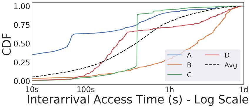
a new cluster of machines), by recording a small number of We show distributions for four arbitrary values of this tag.

Learning on Distributed Traces for Data Center Storage Systems

 Task Entropy Cond.
 Interarrival Time 4.748 3.474
 File Lifetime 7.303 6.575
 Final File Size 3.228 2.538
 R/W Fraction 1.874 1.476

(a) Overall and per-tag value in- (b) Per-task entropy, overall and
terarrival time CDFs. avg. conditioned across all tags. (a) How many CTCs match (b) How often each CTC appears
 across time and clusters. in the data set (one cluster).
Figure 3. Conditioning the distribution on Census tags significantly
reduces entropy, indicating that they are predictive. Figure 4. Transferability (a) and cardinality (b) of Census tags.
There is a visible difference between the distributions de-
 18% of CTCs are observed only once and 2/3 of CTCs are
pending on the specific value, and the average distribution
 observed at most 30 times, pointing to high-cardinality keys.
(the dotted line) captures neither of them. A way to measure
this effect more formally is by computing the information However, many of these tags can still contain information.
entropy of the overall distribution (shown in Figure 3b) and For example, a username may be composed of a partic-
compare it to the conditional entropy (the weighted aver- ular system identifier and a prefix (e.g., “sys_test54” vs.
age over the entropies when conditioning on Census tag “sys_production” ) and table names often have hierarchical
values). The difference between the two is known as the mu- identifiers (e.g., a format such as “type.subtype.timestamp”).
tual information (or information gain), which measures the Only using exactly matching strings would therefore lose
predictiveness of Census Tag collections for the distribution. important information. We need to extract information from
 within these strings, which resembles natural language pro-
Transferability of Census Tags. In order to use Census cessing tasks. Such techniques enable proper information
tags in predictions, we need to show that the information sharing between known values as well as generalization
they provide transfers – i.e., values recorded in one setting to new values that have not been seen before. Of course,
can be used to predict values in a different setting. We are there are also high-cardinality keys that carry little infor-
interested in two particular types of transferability: mation – e.g., unseen UIDs. This has similarities to ML
 applied to code (Karampatsis & Sutton; Shrivastava et al.,
 1. Across time: We want to be able to use past traces to 2020), where tokens are often highly specific to the context
 make predictions months or years in the future. in which they appear.
 2. Across clusters: We want to use traces recorded in
 one cluster to make predictions in other clusters. 3.4 Distribution-based Storage Predictions

For predictions to be transferable, traces must either share Intuitively, we would expect a predictor for the storage pre-
features or have a similar latent structure (e.g., there exists diction tasks from Section 3.2 to predict one value for 
a similar relationship between the keys and values even if (e.g., the expected lifetime of a file) given a CTC . How-
they are named differently). To analyze transferability, we ever, there is inherent uncertainty in these predictions: 1)
conducted a study comparing the keys and values found in features do not always capture all details in the system that
two different clusters and between traces 9 months apart determine the file’s lifetime, and 2) effects outside the con-
(Figure 4a). We find that 1) only a small fraction of requests trol of the system, such as user inputs, affect the predictions.
have a CTC that occurs exactly in the original trace, but 2) For many predictions, there is not a single value that we
most requests have at least one key-value pair that was seen could predict that is correct most of the time. Similar to
in the original trace. This is true both across time and across the work by Park et al. (2018) on cluster scheduling, we
clusters, and indicates that an approach that only records therefore predict a probability distribution of values. This
CTCs in a lookup table will degrade over time and is of lim- distribution can then be consumed by the storage system
ited use across clusters. Meanwhile, it shows that complex directly, similar to EVA (Beckmann & Sanchez, 2017): For
approaches can potentially extract more information. example, a cache could evict a cache entry with a high vari-
 ance in its distribution of interarrival times in favor of an
 entry with low interarrival time at low variance.
High-Cardinality Tags. One example of tags that do not
transfer directly are high-cardinality keys capturing infor- To perform distribution-based predictions, data within the
mation that changes over time or between clusters. For traces needs to be pre-aggregated. Specifically, we need to
example, new accounts or database tables are added over take all entries in the trace with the same X and compute
time and different clusters host different workloads. Tags the distributions for each of the labels Y that we want to
that directly include these identifiers as values will there- predict (interarrival times, lifetimes, etc.). To do so, we can
fore differ. This is visualized in Figure 4b which plots the collect a histogram of these labels for each CTC. We note a
number of times each CTC is observed in a 1.4B entry trace. large skew: Some CTCs appear many orders of magnitude

Learning on Distributed Traces for Data Center Storage Systems

more often than others, and 18% of entries show up only
once (Figure 4b). This can be explained by two effects: 1)
Some systems account for a much larger fraction of requests
than others, and 2) The lower the cardinality of Census tags Figure 5. Fitting lognormal distributions to CTC CDFs.
set by a system, the lower the number of different CTCs
associated with this system.
 are much longer than for other requests. For example, we
 could avoid admitting these entries to the cache at all, or
Fitting Lognormal Distributions. One approach to use prioritize them for eviction.
the histograms for input features is to use them in a lookup
table, which covers low-cardinality cases. However, as we 4 M ACHINE L EARNING FOR C ENSUS TAGS
have seen, some Census Tags have high cardinality and we
therefore need to predict them using models that have the We now demonstrate a set of learning techniques to achieve
ability to generalize to previously unseen values. For these transferability across clusters and over time. We assume that
tags, we therefore need to represent the output distribution all models are compiled and directly linked into the storage
in a way that we can train a model against. server, running either on the CPU, or on an accelerator such
 as a GPU or TPU. When a request is received by a storage
Gaussians (or mixtures of Gaussians) are often used to system, its CTC is represented as an unordered set of string
model this type of output distribution. For example, they are key-value pairs. The prediction problem is formally defined
used for lifetime prediction in survival analysis (Fernandez as follows: Given a CTC , predict the parameters of its
et al., 2016). In particular, we consider lognormal distri- lognormal distribution for a given task, = ( , ).
butions and show that they are a suitable fit for our data.
They are a popular choice for modeling reliability durations
 4.1 Lookup Table Model
(Mullen, 1998). In contrast to other similar distributions
(such as Weibull and log-logistic), the parameters that max- The simplest prediction approach is a lookup table (Figure
imize the lognormal likelihood can be estimated in closed 6a) where a canonical encoding of the CTC is used to index
form. Figure 5 shows examples of fitting lognormals to the a static table that maps CTCs to . The table is “trained” by
pre-aggregated distributions for several CTCs. To measure collecting the target distribution histograms from a training
how well the fitted distributions match the real data, we set, pre-aggregating them, and computing the mean and stan-
use the Kolmogorv-Smirnov (KS) distance, which measures dard deviation of a lognormal distribution that fits the data.
the maximum deviation between CDFs. The overall KS CTCs are encoded by assigning each unique key and value
distance of fitting lognormals to our data is 0.09-0.56. in the training set an ID and looking them up at inference
 time. Keys in the CTC are sorted alphanumerically, ensuring
3.5 Case Study: Database Caching Predictor that the same CTC always results in the same encoding.
We demonstrate the insights from this section using a CTCs not found in the table can be handled by substituting
database system as an example. One Census tag associated the overall distribution of the training set. As shown in
with this system indicates the high-level operation associ- Section 3.3, the entropy of this set is much larger than the
ated with it (Figure 3a). This information can be used to entropy conditioned on a particular CTC (and is therefore
make decisions about admission and eviction. For example, not very predictive), but represents the best we can do. Note
consider values A, C and D of this particular Census tag. that the lookup table can become very large, and it is often
While the average (dotted) CDF of interarrival times for necessary to remove rare CTC entries. There are different
requests increases slowly (note the log scale), indicating ways to implement such a lookup table. For example, it
that the interarrival time is difficult to predict, requests with could be implemented as a hashtable or represented by a
values A/C/D are more predictable: The vertical jump in C decision tree (Safavian & Landgrebe, 1991), which is an
shows that 3/4 of requests with this tag have an interarrival equivalent but potentially more compact representation.
time of 15 minutes, indicating it has a periodicity of 15
minutes. Meanwhile, we see that 2/3 of requests for A take 4.2 K-Nearest Neighbor Model
less than 1 minute before they are accessed again, and for D
 Improving upon how the lookup table handles unseen CTCs,
the same is true for a 5 minutes interval.
 the k-nearest neighbor approach (Figure 6b) makes predic-
We can exploit this information in a caching policy that does tions for these entries by combining predictions from CTCs
not evict these requests for the first 1, 5 and 15 minutes after that are close/similar. We implement an approximate k-NN
their last access. Afterwards, we treat them the same as method that uses as its distance metric the number of differ-
other requests. We can also do something similar for values ing Census Tags between two CTCs. We encode CTCs as
such as B where the distribution shows that interarrival times a sparse binary vector where each entry denotes whether a

Learning on Distributed Traces for Data Center Storage Systems

 each entry will result in a different CTC. This, in turn, means
 that 1) the lookup table grows very large and 2) each entry
 only has a single data point associated with it. Instead of
 a histogram of values, the “distribution” associated with
 (a) Lookup Table Model
 this CTC is therefore a single point mass with = 0. This
 makes it impossible for the model to generalize, since the
 nearest neighbor approach has no way of knowing that the
 different values are identical except for the timestamp.
 (b) Nearest Neighbor Model
 4.3 Neural Network Model
 Handling these high-cardinality cases necessitates a model
 that can parse the strings that constitute the key-value pair.
 While a nearest neighbor approach can learn simple connec-
 tions between predictions and Census tags (e.g., “if tag A
 has value B, the file is short-lived”), it cannot learn more
 complex and non-linear interactions (e.g., "if tag A has an
 even number as value, then the file size is small"). To push
 (c) Embedding-based Transformer
 the limits of learning these more complex connections, we
 use a neural network-based approach. Note that in practice,
 this neural network would not run at every prediction but
 be used as a fall-back for lookup table entries where no
 example can be found (and therefore runs rarely).
 A simple approach would be to encode keys and values
 as IDs (similar to the lookup table), feed them into a
 feed-forward network, and train against the from pre-
 (d) Hierarchical Raw Strings Transformer aggregation. However, this approach still has no capability
 Figure 6. The different models (blue is training).
 to generalize to unseen values nor high-cardinality keys that
 only have a single data point associated with them. We
 address these problems by combining two approaches:
particular Census Tag key-value pair is present. Distance
can thus be cheaply computed as the squared L2 distance 1. We build on recent advances in natural language pro-
between sparse binary vectors (which can reach a dimen- cessing to train networks operating on raw strings.
sionality of millions). This approach allows us to make use Specifically, we use a Transformer (Vaswani et al.,
of existing approximate nearest neighbor libraries that are 2017) model that uses an attention mechanism to con-
highly optimized for sparse vectors. We choose K=50 in our sume a sequence of inputs (e.g., character strings com-
experiments, since binary vectors may have many neighbors prising each Census tag) and maps them to an embed-
of equal distance. For instance, a CTC that has a different ding (i.e., a learned encoding).
value for one Census Tag may get matched against a number 2. To handle CTCs with a single point, we do not train
of CTCs that have distance 2. To compute the predictions, against ( , ) directly, but use Mixture Density Net-
we aggregate the chosen nearest neighbors. The mean is works (Bishop, 1994) to let the model fit a Gaussian.
simply the weighted average over the means of the individ-
 The neural network architecture is based on typical models
ual neighbors. The standard deviation is computed by
 used in NLP to process character and word tokens. We
summing two components: (1) the weighted average over
 present two versions: 1) an embedding-based version that
the variance of each neighbor, and (2) the weighted squared
 resembles the approach above of feeding token-encoded key-
distance between the individual means and the overall mean.
 value pairs directly into the model, and 2) an approach that
This approach resembles strategies that have been used in parses raw strings of key-value pairs. The model architec-
cluster scheduling (Park et al., 2018; Cortez et al., 2017). ture is similar in both cases and relies on learning embedding
In contrast to a lookup table, it has more generalization representations (Mikolov et al., 2013), learned mappings
ability, but it is still unable to extract information from high- from a high-dimensional input to a latent representation in
cardinality Census tags. Imagine a tag where values are of some other – usually lower-dimensional – space.
format .. Here, “query
type” captures information that we want to extract. Since Embedding-Based Transformer Model. For this ver-
“timestamp” will take on a different value for every request, sion (Figure 6c), we start from a CTC = { 1 , 2 , … , }

Learning on Distributed Traces for Data Center Storage Systems

where is the th (unordered) key-value string pair –
encoded as one-hot encoded vectors based on their IDs
– and pass each through a single embedding layer
 ∶ ℕ → ℝ to create a set of embedding vectors
 = { ( 1 ), ( 2 ), … , ( )}. is then passed into the Figure 7. Using the Transformer in multi-task learning.
Transformer encoder ∶ ℝ × → ℝ × and its out-
put is averaged to produce the shared output embedding will be the same, while in cases where we have enough data
 ∑ points, the samples match the distribution.
 = =1 ( ) where ∈ ℝ . Finally, this output
embedding is passed through an additional 2-layer fully
connected network to yield the outputs = ( , ). The Multi-Task Learning. While the Transformer model is
last layer producing uses an ELU activation (specified by shown for a single task, the front-end (encoder) part of the
Mixture Density Networks). model could be reused in a multi-task setup (Figure 7). The
 fully connected layers at the end of the network can be
Hierarchical Raw Strings. This version (Figure 6d) oper- replaced by different layers for each task. The Transformer
ates directly on raw strings, where each character is encoded could then be jointly trained on multiple storage tasks.
as a one-hot vector of dimensionality 128 (127 characters
and one special character to separate key and value). Each 5 I MPLEMENTATION D ETAILS
key-value pair is encoded as a sequence of such one-
hot vectors ( ∈ ℝ ×128 ), and the characters are passed We prototyped and evaluated our models in a simulation
through an embedding layer, yielding an ( ) ∈ ℝ × , setup driven by production traces. We pre-process these
where is the length of the -th key-value pair. Each ( ) traces using large-scale data processing pipelines (Chambers
is then passed through a Transformer encoder – all these et al., 2010) and run them through our models.
encoders’ weights are shared (i.e., this encoder learns how
to parse an individual key-value pair). The outputs of these Lookup Table. The lookup table performance is calcu-
encoders are then passed into another encoder, which now lated using our data processing pipelines. We aggregate
aggregates across the different key-value pairs (i.e., it learns across CTCs, perform predictions for each CTC and then
connections between them). As before, the output is then weight by numbers of requests that belong to each CTC.
averaged and passed through two fully-connected layers.
 K-Nearest Neighbors. We build on the ScaNN nearest-
Mixture Density Networks. Because the goal is to pre- neighbor framework that uses an inverted index method
dict the distribution associated with each CTC, we must for high-performance k-nearest neighbor search (Guo et al.,
choose a loss function that allows the model to appropri- 2020). We use this framework to conduct an offline approx-
ately learn the optimal parameters. Consider if we used imate nearest neighbors search with K=50. Most of this
squared distance to learn the mean and standard deviation pipeline is shared with the lookup table calculation.
of a log-normal distribution. While squared error may be
appropriate for learning the mean, it is not for the standard Transformer. We implement our Transformer models in
deviation. For instance, squared error is symmetric, and TensorFlow (Abadi et al., 2016) and run both training and
underestimating the standard deviation by 0.1 has a much evaluation on TPUs (Jouppi et al., 2017), using the Ten-
larger effect on error than overestimating by 0.1. Addition- sor2Tensor library (Vaswani et al., 2018). We use the
ally, a model trained with squared error will not learn the following hyperparameters: {num_hidden units=64,
correct standard deviation from an overpartitioned dataset num_hidden_layers=2, num_heads=4} and a si-
(e.g., if all CTCs had = 0, the model would learn = 0). nusoid positional embedding. We train using a weighted
Mixture Density Networks (Bishop, 1994) were designed sampling scheme to ensure that CTCs occur approximately
to address this problem. Instead of fitting ( , ) directly as often as they would in the actual trace.
to the label, the predicted ( , ) are used to compute the
likelihood that the label came from this distribution: 6 E VALUATION
 ( [ ])
 1 ( − )2 We evaluate our models on traces. We start with microbench-
 loss = − log √ × exp − marks based on synthetic traces that demonstrate the ability
 2 2 2
 of our models to generalize to unseen CTCs. We then eval-
Note that now instead of training against a distribution , we uate our models on production traces from Google data
need to train against a specific label from this distribution. centers. Finally, we show a simulation study that applies
We therefore sample from at every training step. In our models to two end-to-end storage problems, cache ad-
high-cardinality cases where = 0, all of these samples mission and SSD/HDD tiering.

Learning on Distributed Traces for Data Center Storage Systems

 Tags Len. P/D Samples Table K-NN Transformer
 Separate 2/5 1,000 8.00 0.001 0.008
 requests, we found that after one month, only 0.3% of re-
 Separate 2/5 10,000 8.00 0.000 0.015 quests had CTCs that were never seen before. We measured
 Separate 10 / 20 1,000 8.00 0.000 0.047
 Separate 10 / 20 10,000 8.00 0.000 0.005
 our lookup table at 0.5 s per request and the largest Trans-
 Combined 2/5 1,000 8.00 8.000 0.034 former model at 99 ms (entirely untuned; we believe there
 Combined 2/5 10,000 8.00 8.000 0.003
 Combined 10 / 20 1,000 8.00 8.000 0.017
 is headroom to reduce this significantly). The average la-
 Combined 10 / 20 10,000 8.00 8.000 0.006 tency with the Transformer is therefore 310 s, which is fast
 enough to run at relatively rare operations like file creation
Table 2. Mean squared error (MSE) on a synthetic microbench- (e.g., the SSD/HDD tiering case). For more frequent opera-
mark that combines an information-carrying (P)refix with a
 tions (e.g., block reads/writes), we would use the cheaper
(D)istractor of a certain length, in the same or separate tags.
 models, whose latency can be hidden behind disk access.
6.1 Microbenchmarks
 6.3 Production Traces
To demonstrate the ability of our models to learn informa-
 We now evaluate our models on real production traces. Our
tion in high-cardinality and free-form Census tag strings,
 evaluation consists of two main components: evaluating
we construct a synthetic data set for the interarrival time
 model generalization error, and demonstrating end-to-end
task. We create 5 overlapping Gaussian clusters with means
 improvements in simulation.
 = {1, 3, 5, 7, 9} and = 1. Requests from the same clus-
ter are assigned a shared prefix and a randomly generated As discussed in Section 3.3, we would like models to gen-
distractor string (in real Census tags, this might be a times- eralize 1) across long time horizons, and 2) across clusters.
tamp or UID). The goal is for the model to learn to ignore We train models on a 3-month trace and evaluate their gener-
the distractor string and to predict the parameters of each alization on a 3-month trace from the same cluster 9 months
cluster based on the observed shared prefix. We experiment later, and a 3-month trace from the same time period on a
with two different setups: 1) the prefix and distractor are different cluster. We find that models perform well within
in separate Census tags, and 2) the prefix and distractor the same cluster and less (though acceptably) well across
are combined in the same Census tag. For the former, the clusters. We measure both the weighted and unweighted
model has to learn to ignore one particular Census tag, for error, and show that simple models are sufficient to learn the
the latter, it has to extract part of a string. head of the distribution while more complex models are bet-
 ter at modeling the long tail. We also find that while there is
We compute the MSE to indicate how close the predicted
 some drift in each CTC’s intrinsic statistics, generalization
log-normal parameters ( , ) were to the ground truth. An
 error across time is largely due to unseen CTCs, indicating
error of 0 indicates that we perfectly recovered the distri-
 that a model can be stable over time. More details about the
bution, while an error of 8 (= (2 × 22 + 2 × 42 + 0)∕5)
 results and error metrics can be found in the Appendix.
corresponds to always predicting the average of all means.
We also vary the number of samples per cluster between
 6.4 End-to-End Improvements
1,000 and 10,000 to study how many samples are needed to
learn these parameters. The lookup table is unable to learn We now show two case studies to demonstrate how the CDF
either case, since it can only handle exactly matching CTCs predictions can be used to improve storage systems. While
(Table 2). K-Nearest Neighbor (with K=∞) can correctly our simulations use production traces and are inspired by
predict the separate cases, but fails on the combined cases realistic systems, they are not exact representations of any
since it cannot look into individual strings. Finally, the neu- real Google workload. Additional evaluation of variation
ral network successfully learns all cases. We find that 10K within some of these results is provided in the Appendix.
samples per class were sufficient to learn a predictor that
stably achieves an error close to 0 and does not overfit. This
data shows how our models are able to learn successively Cache Admission and Eviction. We implement a cache
more information, representative of the actual traces. simulator driven by a consecutive time period of 40M read
 requests from our production traces. These are longitudinal
 traces to a distributed file system; while our simulation does
6.2 Prediction Latency
 not model any specific cache in our production system, this
A key question for deployment is the models’ latency. In is equivalent to an in-memory cache in front of a group of
practice, the lookup table will be used to cover the vast servers that are handling the (small) slice of files represented
majority of cases and the more expensive models only run by our traces. Such caches can have a wide range of hit
when a CTC is not in the table (the result is added for the rates (Albrecht et al., 2013), depending on the workload mix
next time the CTC is encountered). This gives the best and upstream caches. As such, these results are representa-
of both worlds – resilience to drift over time and across tive for improvements one might see in production systems.
clusters, and high performance. Evaluating on file creation The approach is similar to prior work on probability-based

Learning on Distributed Traces for Data Center Storage Systems

 with an SSD tier to reduce HDD disk I/O utilization (since
 spinning disks are limited by disk seeks, fewer accesses for
 hot and short-lived data means that fewer disks are required).
 Our baseline is a policy that places all files onto SSD initially
 and moves them to HDD if they are still alive after a specific
 TTL that we vary from 10s to 2.8 hours. We use 24 hours
 (a) Calculating Utility (b) Cache Hit Rate of the same traces as in the previous example and compute
 the average amount of live SSD and HDD memory, as well
 Figure 8. Using predictions in caching.
 as HDD reads and (batched) writes as a proxy for the cost.
 We use our model to predict the lifetime of newly placed
 files (Figure 9). We only place a file onto SSD if the pre-
 dicted + × is smaller than the TTL (we vary = 0, 1).
 After the file has been on SSD for longer than + × 
 ( = 1, 2), we move it to the HDD. This reduces write I/O at
 Figure 9. Using predictions in SSD/HDD tiering. the same SSD size (e.g., by ≈20% for an SSD:HDD ratio of
 1:20) or saves SSD bytes (by up to 6×), but did not improve
replacement policies such as EVA (Beckmann & Sanchez, reads. We also used the model to predict read/write ratio
2017) or reuse interval prediction (Jaleel et al., 2010). The (Section 3.2) and prefer placing read-heavy files on SSD.
main difference is that we can predict these reuse intervals This keeps the write savings while also improving reads.
more precisely using application-level features.
We consider a cache that operates at a 128KB fixed block 7 F UTURE W ORK
size granularity and use an LRU admission policy as the
baseline; LRU is competitive for our distributed file system Systems Improvements. The caching and storage tiering
caching setup, similar to what is reported by Albrecht et al. approach has applications across the entire stack, such as
(2013). Our learning-based policy works as follows: At selecting local vs. remote storage, or DRAM caching. Other
every access, we use our model to predict ( , ) of the prediction tasks in storage systems that can benefit from
lognormal distribution associated with this request. We store high-level information include read-write ratio, resource
these parameters in the block’s metadata, together with the demand forecasting, and antagonistic workload prediction.
timestamp of the last access to the block. We now define the Our approach could also be applied to settings other than
utility of a block as the probability that the next access to storage systems (e.g., databases), and to other (non-Census)
the block is within the next Δ = 1,000s (Δ is configurable). meta-data, such as job names.
This value can be computed in closed-form (Figure 8a):
 CDF( + Δ | , ) − CDF( | , ) Modeling Improvements. Our approach could benefit
 Utility( , , ) =
 1 − CDF( | , ) from a method for breaking up Census Tags into meaningful
 sub-tokens. In addition to the bottom-up compression-based
We logically arrange the blocks into a priority queue sorted
 approaches used in NLP such as Byte Pair Encoding (BPE,
by increasing utility. When we insert a block into the cache,
 Gage (1994)) or WordPiece (Wu et al., 2016), we may also
we compute its utility and add it to the priority queue. If we
 want to identify known important tokens ahead of time, e.g.
need to evict a block, we pick the entry at the front of the
 “temp” or “batch”. This would improve our model’s abil-
queue (after comparing it to the utility of the new block).
 ity to generalize to unseen Census Tags and new clusters.
We therefore ensure that we always evict the block with the
 On the distribution fitting side, log-normal distributions are
lowest utility/probability of access. Note that this utility
 not ideal in all scenarios. For instance, distributions that
changes over time. Recomputing all utilities and sorting the
 are bounded or multi-modal are respectively better handled
priority queue at every access would be prohibitive – we
 using a Beta distribution or Mixture-of-Gaussians.
therefore only do so periodically (e.g., every 10K requests).
An alternative is to continuously update small numbers of
entries and spread this work out across time. Figure 8b 8 C ONCLUSION
shows that the model improves the hit rate over LRU by as
 Our results demonstrate that information in distributed
much as from 17% to 30%.
 traces can be used to make predictions in data center storage
SSD/HDD Tiering: We perform a simple simulation study services. We demonstrated three models – a lookup ta-
to demonstrate how predictions can be used to improve ble, k-NN and neural-network based approach – that, when
SSD/HDD tiering. We assume a setup similar to Janus combined, extract increasing amounts of information from
(Albrecht et al., 2013) where an HDD tier is supplemented Census tags and significantly improve storage systems.

Learning on Distributed Traces for Data Center Storage Systems

ACKNOWLEDGEMENTS Chang, F., Dean, J., Ghemawat, S., Hsieh, W. C., Wallach,
 D. A., Burrows, M., Chandra, T., Fikes, A., and Gruber,
We want to thank Richard McDougall for supporting this R. E. Bigtable: A distributed storage system for structured
project since its inception and providing us with invaluable data. ACM Transactions on Computer Systems (TOCS),
feedback and technical insights across the storage stack. 26(2):4, 2008.
We also want to thank David Andersen, Eugene Brevdo,
Andrew Bunner, Ramki Gummadi, Maya Gupta, Daniel Corbett, J. C., Dean, J., Epstein, M., Fikes, A., Frost, C.,
Kang, Sam Leffler, Elliot Li, Erez Louidor, Petros Maniatis, Furman, J. J., Ghemawat, S., Gubarev, A., Heiser, C.,
Azalia Mirhoseini, Seth Pollen, Yundi Qian, Colin Raffel, Hochschild, P., et al. Spanner: Google’s globally dis-
Nikhil Sarda, Chandu Thekkath, Mustafa Uysal, Homer tributed database. ACM Transactions on Computer Sys-
Wolfmeister, Tzu-Wei Yang, Wangyuan Zhang, and the tems (TOCS), 31(3):8, 2013.
anonymous reviewers for helpful feedback and discussions.
 Cortez, E., Bonde, A., Muzio, A., Russinovich, M., Fon-
 toura, M., and Bianchini, R. Resource central: Under-
R EFERENCES standing and predicting workloads for improved resource
Abadi, M., Barham, P., Chen, J., Chen, Z., Davis, A., management in large cloud platforms. In Proceedings
 Dean, J., Devin, M., Ghemawat, S., Irving, G., Isard, M., of the 26th Symposium on Operating Systems Principles,
 Kudlur, M., Levenberg, J., Monga, R., Moore, S., Murray, SOSP ’17, pp. 153–167, New York, NY, USA, 2017.
 D. G., Steiner, B., Tucker, P., Vasudevan, V., Warden, P., Association for Computing Machinery. URL https:
 Wicke, M., Yu, Y., and Zheng, X. Tensorflow: A system //doi.org/10.1145/3132747.3132772.
 for large-scale machine learning. In 12th USENIX Sympo-
 Delimitrou, C. and Kozyrakis, C. Quasar: Resource-
 sium on Operating Systems Design and Implementation
 efficient and qos-aware cluster management. In Pro-
 (OSDI 16), pp. 265–283, Savannah, GA, November 2016.
 ceedings of the 19th International Conference on Ar-
 USENIX Association. URL https://www.usenix.
 chitectural Support for Programming Languages and
 org/conference/osdi16/technical-
 Operating Systems, ASPLOS ’14, pp. 127–144, New
 sessions/presentation/abadi.
 York, NY, USA, 2014. Association for Computing
Albrecht, C., Merchant, A., Stokely, M., Waliji, M., Machinery. URL https://doi.org/10.1145/
 Labelle, F., Coehlo, N., Shi, X., and Schrock, E. 2541940.2541941.
 Janus: Optimal flash provisioning for cloud storage
 workloads. In Proceedings of the USENIX Annual Devlin, J., Chang, M.-W., Lee, K., and Toutanova, K. Bert:
 Technical Conference, pp. 91–102, 2560 Ninth Street, Pre-training of deep bidirectional transformers for lan-
 Suite 215, Berkeley, CA 94710, USA, 2013. URL guage understanding. arXiv preprint arXiv:1810.04805,
 https://www.usenix.org/system/files/ 2018.
 conference/atc13/atc13-albrecht.pdf. Fernandez, T., Rivera, N., and Teh, Y. W. Gaussian
Barham, P., Isaacs, R., Mortier, R., and Narayanan, D. Mag- processes for survival analysis. In Advances in
 pie: Online modelling and performance-aware systems. Neural Information Processing Systems 29, pp. 5021–
 In Proceedings of the 9th Conference on Hot Topics in 5029. Curran Associates, Inc., 2016. URL http:
 Operating Systems - Volume 9, 2003. //papers.nips.cc/paper/6443-gaussian-
 processes-for-survival-analysis.pdf.
Beckmann, N. and Sanchez, D. Maximizing cache perfor-
 mance under uncertainty. In 2017 IEEE International Fitzpatrick, B. Distributed caching with memcached. Linux
 Symposium on High Performance Computer Architecture journal, 2004(124):5, 2004.
 (HPCA), pp. 109–120, 2017.
 Gage, P. A new algorithm for data compression. The C
Bishop, C. M. Mixture density networks. 1994. URL Users Journal, 12(2):23–28, 1994.
 http://publications.aston.ac.uk/id/
 eprint/373/. Gan, Y., Zhang, Y., Cheng, D., Shetty, A., Rathi, P., Katarki,
 N., Bruno, A., Hu, J., Ritchken, B., Jackson, B., Hu,
Chambers, C., Raniwala, A., Perry, F., Adams, S., Henry, K., Pancholi, M., He, Y., Clancy, B., Colen, C., Wen,
 R., Bradshaw, R., and Nathan. Flumejava: Easy, efficient F., Leung, C., Wang, S., Zaruvinsky, L., Espinosa, M.,
 data-parallel pipelines. In ACM SIGPLAN Conference Lin, R., Liu, Z., Padilla, J., and Delimitrou, C. An
 on Programming Language Design and Implementation open-source benchmark suite for microservices and their
 (PLDI), pp. 363–375, 2 Penn Plaza, Suite 701 New York, hardware-software implications for cloud edge systems.
 NY 10121-0701, 2010. URL http://dl.acm.org/
 citation.cfm?id=1806638.

Learning on Distributed Traces for Data Center Storage Systems

 In Proceedings of the Twenty-Fourth International Con- Wilcox, E., and Yoon, D. H. In-datacenter performance
 ference on Architectural Support for Programming Lan- analysis of a tensor processing unit. SIGARCH Com-
 guages and Operating Systems, ASPLOS ’19, pp. 3–18, put. Archit. News, 45(2):1–12, June 2017. URL https:
 New York, NY, USA, 2019a. Association for Computing //doi.org/10.1145/3140659.3080246.
 Machinery. URL https://doi.org/10.1145/
 3297858.3304013. Kanev, S., Darago, J. P., Hazelwood, K., Ranganathan, P.,
 Moseley, T., Wei, G.-Y., and Brooks, D. Profiling a
Gan, Y., Zhang, Y., Hu, K., Cheng, D., He, Y., Pancholi, warehouse-scale computer. ACM SIGARCH Computer
 M., and Delimitrou, C. Seer: Leveraging big data to Architecture News, 43(3):158–169, 2016.
 navigate the complexity of performance debugging in
 cloud microservices. In Proceedings of the Twenty-Fourth Karampatsis, R.-M. and Sutton, C. Maybe deep neural
 International Conference on Architectural Support for networks are the best choice for modeling source code.
 Programming Languages and Operating Systems, AS- arXiv preprint arXiv:1903.05734.
 PLOS ’19, pp. 19–33, New York, NY, USA, 2019b. Kim, T., Hahn, S. S., Lee, S., Hwang, J., Lee, J., and
 Association for Computing Machinery. URL https: Kim, J. Pcstream: Automatic stream allocation us-
 //doi.org/10.1145/3297858.3304004. ing program contexts. In 10th USENIX Workshop
Ghemawat, S., Gobioff, H., and Leung, S.-T. The google on Hot Topics in Storage and File Systems (HotStor-
 file system. In Proceedings of the 19th ACM Symposium age 18), Boston, MA, July 2018. USENIX Association.
 on Operating Systems Principles, 2003. URL https://www.usenix.org/conference/
 hotstorage18/presentation/kim-taejin.
Guo, R., Sun, P., Lindgren, E., Geng, Q., Simcha, D., Chern,
 F., and Kumar, S. Accelerating large-scale inference Kirilin, V., Sundarrajan, A., Gorinsky, S., and Sitaraman,
 with anisotropic vector quantization. In International R. K. Rl-cache: Learning-based cache admission for
 Conference on Machine Learning, 2020. URL https: content delivery. In Proceedings of the 2019 Work-
 //arxiv.org/abs/1908.10396. shop on Network Meets AI ML, NetAI’19, pp. 57–63,
 New York, NY, USA, 2019. Association for Computing
Hochreiter, S. and Schmidhuber, J. Long short-term memory. Machinery. URL https://doi.org/10.1145/
 Neural computation, 9(8):1735–1780, 1997. 3341216.3342214.
Howard, J. H., Kazar, M. L., Menees, S. G., Nichols, D. A., Liu, E., Hashemi, M., Swersky, K., Ranganathan, P., and
 Satyanarayanan, M., Sidebotham, R. N., and West, M. J. Ahn, J. An imitation learning approach for cache re-
 Scale and performance in a distributed file system. ACM placement. In III, H. D. and Singh, A. (eds.), Proceed-
 Transactions on Computer Systems (TOCS), 6(1):51–81, ings of the 37th International Conference on Machine
 1988. Learning, volume 119 of Proceedings of Machine Learn-
Jaleel, A., Theobald, K. B., Steely, S. C., and Emer, J. High ing Research, pp. 6237–6247. PMLR, 13–18 Jul 2020.
 performance cache replacement using re-reference inter- URL http://proceedings.mlr.press/v119/
 val prediction (rrip). SIGARCH Comput. Archit. News, liu20f.html.
 38(3):60–71, June 2010. URL https://doi.org/ Mikolov, T., Chen, K., Corrado, G., and Dean, J. Efficient
 10.1145/1816038.1815971. estimation of word representations in vector space. arXiv
Jouppi, N. P., Young, C., Patil, N., Patterson, D., Agrawal, preprint arXiv:1301.3781, 2013.
 G., Bajwa, R., Bates, S., Bhatia, S., Boden, N., Borchers,
 Mullen, R. E. The lognormal distribution of software failure
 A., Boyle, R., Cantin, P.-l., Chao, C., Clark, C., Coriell,
 rates: application to software reliability growth modeling.
 J., Daley, M., Dau, M., Dean, J., Gelb, B., Ghaem-
 In Proceedings Ninth International Symposium on Soft-
 maghami, T. V., Gottipati, R., Gulland, W., Hagmann,
 ware Reliability Engineering (Cat. No.98TB100257), pp.
 R., Ho, C. R., Hogberg, D., Hu, J., Hundt, R., Hurt,
 134–142, 1998.
 D., Ibarz, J., Jaffey, A., Jaworski, A., Kaplan, A., Khai-
 tan, H., Killebrew, D., Koch, A., Kumar, N., Lacy, S., OpenCensus. Opencensus. https://opencensus.
 Laudon, J., Law, J., Le, D., Leary, C., Liu, Z., Lucke, io/, 2020. URL https://opencensus.io/.
 K., Lundin, A., MacKean, G., Maggiore, A., Mahony,
 M., Miller, K., Nagarajan, R., Narayanaswami, R., Ni, Ousterhout, J., Gopalan, A., Gupta, A., Kejriwal, A., Lee,
 R., Nix, K., Norrie, T., Omernick, M., Penukonda, N., C., Montazeri, B., Ongaro, D., Park, S. J., Qin, H., Rosen-
 Phelps, A., Ross, J., Ross, M., Salek, A., Samadiani, E., blum, M., Rumble, S., Stutsman, R., and Yang, S. The
 Severn, C., Sizikov, G., Snelham, M., Souter, J., Stein- ramcloud storage system. ACM Trans. Comput. Syst.,
 berg, D., Swing, A., Tan, M., Thorson, G., Tian, B., 33(3), August 2015. URL https://doi.org/10.
 Toma, H., Tuttle, E., Vasudevan, V., Walter, R., Wang, W., 1145/2806887.