Monetary Capacity Roberto Bonfatti, University of Padua and University of Nottingham Adam Brzezinski, University of Oxford K. Kivanc Karaman ...
←
→
Page content transcription
If your browser does not render page correctly, please read the page content below
Monetary Capacity

Roberto Bonfatti, University of Padua and University of Nottingham
                     Adam Brzezinski, University of Oxford
                    K. Kivanc Karaman, Bogazici University
             Nuno Palma, University of Manchester and CEPR

                                  November 14, 2019

                                          Abstract

   The monetization of an economy and its fiscal capacity move together in the long run.
We provide historical evidence in support of this proposition, and propose a model that
explains it. The model shows that while monetization and fiscal capacity are substitutes
in the short run, they are complements in the long run. This is because highly monetized
societies generate stronger incentives for governments to invest in fiscal capacity, but in turn
high fiscal capacity makes it easier for governments to commit to monetary stability, thus
leading to higher monetization. We provide case-study evidence in support of our mecha-
nism, focusing on early successes such as eighteenth and nineteenth century Britain, and
failures, such as Ming China. We conclude by discussing implications for macroeconomics
and development.
   JEL Codes: E50, E60, H21, N10, O11
   Keywords: Historical money supply, fiscal capacity, fiscal theory of the price level

                                               1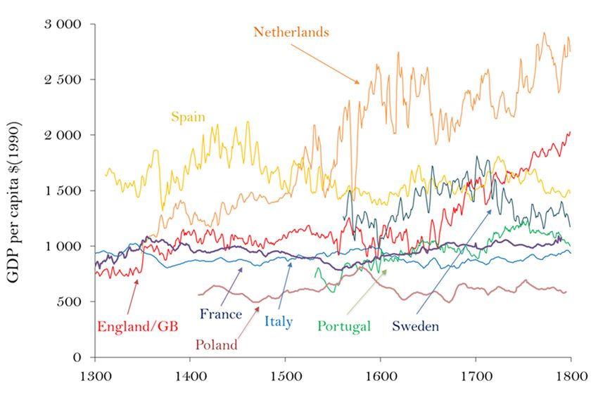
1     Introduction
Even a cursory reading of history provides abundant evidence that the ups and downs of the fiscal
capacity of a state overlapped with the fortunes of its monetary unit. While fiscally troubled
states failed to issue and circulate money, declining monetization was usually associated with
a decrease in tax revenues and the collapse of government authority. Beyond the anecdotal
evidence, however, there is little systematic work to document the relationship between monetary
and fiscal capacity, formally model the underlying causal mechanisms, and empirically identify
the causal effects.
    This paper contributes to the literature on each of these three fronts. It provides a bird’s eye
view of the co-evolution of fiscal and monetary capacity across Europe from the 16th to 19th
century, as well as giving more detailed accounts of this relationship for several states. As for
the mechanics of this relationship, it models how greater monetization made taxation easier and
induced states to invest in fiscal capacity, and how greater fiscal capacity induced monetization by
allowing states to commit to refrain from predatory monetary policies. Empirically, it estimates
the causal impact of monetization on the rise in fiscal capacity in Europe, relying on the natural
experiment offered by the massive inflow of silver after the discovery of the New World. All in
all, we find that money was not neutral in the long run and had major implications for political
and economic development.
    Figure 1 provides a long run view of the relationship between monetary and fiscal capacity.
Monetary capacity refers to a state’s capacity to issue and circulate sufficient liquidity for the
functioning of markets. We proxy it by real money stock per capita. Fiscal capacity refers to a
state’s capacity to extract revenues and mobilize resources to implement its policies. We proxy
it by real tax revenues per capita.1 The figure plots the real money stock per capita on the
horizontal and real tax revenues per capita on the vertical axis for eight major European states
   1
     Fiscal capacity is defined as the capacity to collect taxes, but the proxy is the actual tax collection, and
the two are not necessarily equal. The political preferences of the government can dictate a tax rate lower than
what state’s fiscal and bureaucratic apparatus can potentially collect. For example, states in developed countries
today choose to collect less taxes than they potentially can. For the period we investigate, however, the difference
between actual and potential tax collection is likely to be small. Early Modern states had weak bureaucracies and
a weak hold on domestic monopoly of violence. For most states in most years, it was the fiscal capacity rather
than political preferences that was the binding constraint on the actual tax collection.

                                                         2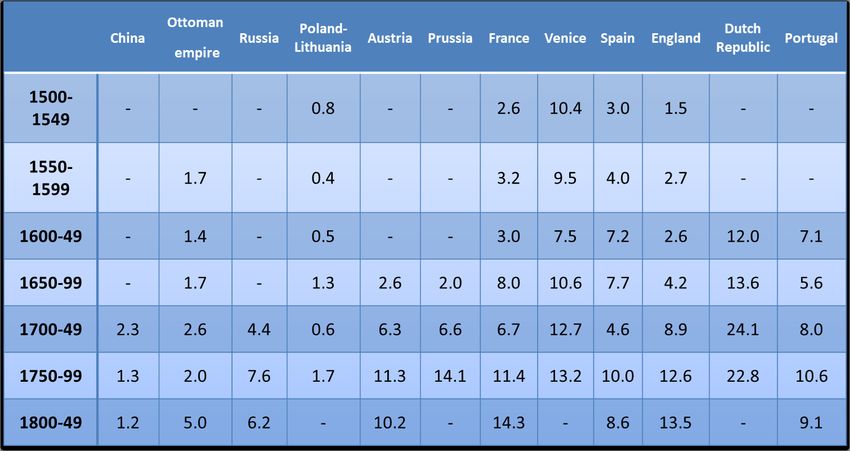
Figure 1: Real tax revenues and money stock per capita. Sources: see text

between 1500 and 1900. The pattern that emerges is a close positive relationship between the
two, with high tax revenue states also boasting high per capita real money balances.
   To unravel the mechanics of this close relationship, we introduce a model that builds on two
insights. The first is that the public accepted state-issued money only to the extent that the state
could commit to refrain from deflating it. In practice, this required the state to develop credible
revenue sources to meet negative fiscal shocks, so that it would not need to seek seigniorage
revenue. The second insight is that monetization eased the collection and administration of
taxes. It eased the collection, because monetization expanded market activity, and markets were

                                                  3
easier to monitor and tax than nonmarket activities. Monetization also eased the administration,
because once collected, money taxes could be conveniently transported around the country and
administered in centralized way, whereas taxes in kind could not.
In a two-period model, we show that these two insights together imply a mutually reinforcing
relationship between monetary and fiscal capacity. On the one hand, monetization induced a
state to invest in fiscal capacity by expanding its fiscal apparatus and bureaucracy, as it was
easier to tax a monetized economy. On the other, fiscal capacity made it feasible to meet future
fiscal shocks by raising taxes, and made states less dependent on seigniorage. This implicit
commitment to refrain from seeking seigniorage revenue in turn induced the public to hold
more money. In equilibrium, monetary and fiscal capacity moved together. Furthermore, any
exogenous increase or disruption in monetary capacity spilled over to fiscal capacity, and vice
versa.
We test the implications of the model relying on what was arguably the most significant
exogenous shock to monetary capacity in history: the inflow of silver and gold from the New
World. Using the exogenous variation in money supply generated by arrival of precious metals,
we find evidence for a strong and significant effect of monetary on fiscal capacity for our sample
of early modern economies. In England, the country with the most complete data, a 1 percent
increase in monetary capacity led to an increase of at least 0.4 percent after two to three decades.
These findings offer new insights on several central ideas in macroeconomics, including the
quantity theory of money. Quantity theory predicts that an increase in money supply has no
real effects, and only leads to a proportionate increase in the price level. The common wisdom
in the literature is that quantity theory holds in the long run.2 In contrast, we find that the
increase in money supply did have a real effect, in the form of an increase in fiscal capacity. The
reason we get this positive effect is that before the exogenous silver shock to the money supply,
large segments of the Feudal economy were not sufficiently monetized and lacked liquidity. When
silver arrived, and the money supply expanded, money penetrated into these under-monetized
segments and provided liquidity. Prices increased, but less than proportionally, because now,
2
The short term effects of money, on the other hand, are well-documented. For historical evidence, see
Brzezinski et al. (2019), Palma (2019) and Velde (2009).
4a greater share of the economic activity relied on money. The growing monetization in turn
facilitated expansion of market activity, an increase in tax collection and the collapse of feudal
structures. Hence, the effects of the increase in money supply were real, and significant.
The findings also relate to the fiscal theory of the price level. According to this theory, states
can raise revenue either by increasing taxes or increasing money supply, the latter of which in
turn increases the price level. Hence, in the short run, taxes and monetary expansion are modeled
as substitutes. We find in this study that over the long run the relationship was more complex.
In under-monetized economies, if the money supply expanded in a way that provided liquidity
to new regions or sectors, it improved tax collection, and triggered a virtuous cycle of monetary
and fiscal capacity building. Hence, in the long run, taxes and monetary expansion acted as
complements.
Finally, the co-evolution of fiscal and monetary capacity matters, because both of them also
affected economic performance. Fiscal capacity allowed states to integrate domestic markets and
expand overseas, provide public goods, and solve externality problems. It also promoted growth
by financing legal capacity and protecting property rights.3 Monetary capacity, on the other
hand, was a public good that pervaded all sectors of the economy and facilitated market activity.
It lowered transaction costs, and facilitated trade and investment.4 Hence, the simultaneous
increase in fiscal and monetary capacity in early modern Europe also helps explain why Europe
surged ahead economically.
2 Model
Consider an economy inhabited by a multitude of agents, which lasts for two periods. All private
agents have the same exogenously given income, which is equal to y in both periods. Preferences
are linear in consumption, as well as in a public good provided by the government. While
consumption receives weight one in preferences, the public good receives weight α > 1. In each
period s ∈ {1, 2}, up to an amount γs ms y of the public good can be provided, where ms is an
endogenous variable to be described below, and γs is a random variable which takes value γ > 0
3
Besley and Persson (2011)
4
Irigoin (2009a,b, 2013)
5with probability π, and value zero with probability 1 − π. The public good can be interpreted
as expenditure in defence, and the case γs = γ as one in which, in period s, the country must
fight an external war.
Income can be seen as the sum of the value added generated in a multitude of transactions
taking place in each period. A share ms ∈ [0, 1] of these transactions is conducted using money,
as opposed to barter. In period 1, this share is exogenously given. The share for period 2 is
determined by agents at the end of period 1.
We have assumed that the maximum expenditure in the public good, γs ms y, is proportional
to the degree of monetization of the economy (ms ), and to the economy’s size (y). As clarified
below, this assumption simplifies the model by ensuring that expenditures are proportional to
revenues.5
In each period, the government can generate an inflation tax is ∈ [0, 1], inflicting a loss is ms y
on private agents, and giving the government revenues δis ms y. For example, if money is paper
money, the government could print new money. Of, if money is metallic, the government could
impose a debasement of the existing currency, either by forcing agents to bring their coins to the
mint for re-minting, or by providing incentives to do so.6
We assume 1/α < δ < 1. The second inequality means that the inflation tax inflicts a
higher cost on private agents than it generates revenues for the government. As clarified below,
this will imply that the inflation tax is more inefficient than general taxation. One justification
for this might be that an inflation tax reduces the reputation of the government as a monetary
authority, thus compromising its future ability to generate revenues.7 The first inequality ensures
5
While this assumption simplifies the model, it is not strictly required to generate our results.
6
For example, the government could allow for the production of currency units (e.g. francs, ducats, etc) with
a lower metal content. Agents would then bring their currency units to the mint, to obtain a higher number of
units. In the process, the government could reduce the metal content of the currency units more than initially
declared, thus keeping part of the metal for itself.
7
Without these dynamic considerations, it is not obvious why an inflation tax should be more inefficient than
general taxation. Suppose for example that yt Pt = vt Mt holds, where Mt is money supply and vt is the velocity
of money. Suppose yt = vt = 1 for all t. Suppose that the government increases the money supply from M1 = 100
to M2 = 120, in the process appropriating 10 units of the newly minted currency. The wealth of agents decreases
from M1 /P1 = 100/100 = 1 to M2 /P2 = 110/120 = 0.9167, while the government gains 10/P2 = 0.8333. Clearly,
in this case, the inflation tax inflicts the same cost on private agents than it generates revenues for the government.
One could alternatively justify the assumption by arguing that re-minting is costly, but administering a general
taxation system is costly, too.
6that, despite its inefficiency, money-printing is desirable as a last-resort source of public revenues
in case of war.
Agents choose m2 based on their expectation on the inflation tax that the government will
impose in period 2, ie2 . We capture this in reduced form,8 by assuming
m2 = m (ie2 , µ) ,
where m (0, µ) > 0, m (1, µ) = 0, and the function m is decreasing and concave in ie2 : it is
dm/die2 < 0, d2 m/d (ie2 )2 < 0. In words, the negative effect of an increase in expected inflation
on monetization is smaller at low levels of expected inflation.9 The parameter µ ≥ 0 is a shifter
capturing all exogenous factors that facilitate the monetization of the economy. A rise in µ could
capture, for example, a rise in the amount of available metal. It is ∂m/∂µ > 0, ∂ 2 m/∂ie2 ∂µ ≤ 0
and ∂ 2 m/∂µ∂ie2 ≤ 0.10
The government can also impose a tax ts on the value added generated in transactions. We
want to capture the idea that transactions denominated in money are easier to tax. We obtain this
by assuming that only transactions denominated in money can possibly be taxed. Alternatively,
one could assume that all transactions can be taxed, but transactions not denominated in money
require greater fiscal capacity to tax.11 In each period, the tax cannot exceed the state’s current
fiscal capacity, τs . Fiscal capacity in period 1 is exogenously given, while fiscal capacity in period
2 is determined by the government in period 1. To increase fiscal capacity to τ2 > τ1 costs
φF (τ2 − τ1 ), where F is an increasing and convex function, with F 0 (0) = 0, F 0 (1 − τ1 ) = ∞.
To obtain a unique solution (see below), we further assume F 000 (0) > 0. The parameter φ > 0
8
The function m could be micro-founded using a monetary model such as in Ch. 24 of Ljungqvist and Sargent
(2004). Note that in those models the government can freely chose the money supply. Instead, we would have
to assume that the money supply is ultimately constrained by the amount of metal in circulation. By increasing
such amount, the inflow of metal from the colonies would presumably lead to higher monetization, as we assume
below.
9
This assumption helps ensuring the uniqueness of the equilibrium, but would ultimately have to be justified
by a micro-founded model.
10
So, an increase in µ rotates the function m upwards, increasing the intercept on the y axis but leaving the
intercept on the x axis unchanged.
11
The simplest way to model this would be assuming that the cost of investment in fiscal capacity F (see
below) is increasing in mt . Note that one potential issue with the current formulation is that with transactions
denominated in money being easier to tax, m2 will also be a decreasing function of te2 in a micro-founded model.
7is a cost shifter that captures all exogenous factors that make investment in fiscal capacity less
attractive.
Indirect utility in period s is equal to
vs = αgs + [1 − (is + ts ) ms ] y.
In each period, the government maximises expected inter-temporal utility subject to a bal-
anced budget constraint and to the other constraints described above. The discount rate is equal
to one.
The timing of the game is as follows:
• Period 1:
1.1 The government sets t1 and i1 .
1.2 The government sets τ2 .
1.3 Private agents set m2 . The public good is produced, payoffs realise.
• Period 2: The government sets t2 and i2 . The public good is produced, payoffs realise.
We solve for the equilibrium using backward induction.
Period 2. Assume min [δ + τ2 , 1] > γ > τ2 .12 This means that, even in the “war scenario”,
the government is able to provide the efficient amount of the public good, however it must
resort to money printing to some extent. This assumption generates a “static substitutability”
between taxes and monetary expansion, as in standard fiscal theories of the price level. However,
we show below that, dynamically, taxes and monetary expansion (more precisely, the degree of
monetization) are complements, because a higher degree of monetization makes it more attractive
to invest in fiscal capacity.
Because taxes and monetary expansion are substitutes, investment in fiscal capacity acts as
an implicit commitment device: the greater fiscal capacity, the lesser the need to resort to money
printing in case of war.
12
Although τ2 is endogenous, it is always possible to choose γ so that it falls in the required range. Alternatively,
as evident from the first order condition below, one can always choose τ1 (which is exogenous) and φ so that the
equilibrium τ2 is just below γ, thus making the assumption true.
8The government’s problem is
max αg2 + [1 − (i2 + t2 ) m2 ] y s.t.
i2 ,t2
(δi2 + t2 ) m2 y = g2
t2 ≤ τ2
g2 ≤ γ2 m2 y
If γ2 = 0, there is no need to spend on public goods. The government will then set t2 = i2 = 0.
If γ2 = γ, the government wants to raise γm2 y in revenues. Given that money-printing is a less
efficient source of revenues than taxes, the government first sets taxes to the highest possible
level, t2 = τ2 , and finance the rest of the cost of providing public goods through money printing,
γ − τ2
i2 = .
δ
Period 1. In period 1.3, forward looking agents set
γ − τ2
m2 = m π ,µ .
δ
Note that a higher fiscal capacity in period 2 encourages private agents to hold more money in
that period: this is the commitment mechanism described above.
Consider investment in fiscal capacity in period 1.2. Suppose for simplicity that γ1 = 0,
so that revenues in period 1 are allocated entirely to investment in fiscal capacity. Also for
simplicity, suppose that fiscal capacity in period 1 is large to enough to pay for the optimal
investment in fiscal capacity in period 2. Clearly, the government will then chose a level of tax
that is just enough to pay for investment in fiscal capacity t1 = F (τ2 − τ1 ) / (m1 y)
After some manipulations (reported in the Appendix), the government’s problem can be
9written as
(δα − 1) γ + (1 − δ) τ2 γ − τ2
max y − φF (τ2 − τ1 ) + y + π m π ,µ .
τ2 δ δ
The solution to this problem satisfies the first order condition
I II
z }| { z }| {
1−δ γ − τ2 (δα − 1) γ + (1 − δ) τ2 ∂m
π m π ,µ +π − e = φF 0 (τ2 − τ1 ) , (1)
δ δ δ2 ∂i2
which has a unique solution.13
Our main result is contained in the following Proposition:
Proposition 1. A fall in φ and a rise in µ both lead to a greater fiscal capacity and a higher
monetization of the economy in period 2 (higher τ2∗ and m2 ).
Proof. In the Appendix.
The parameters φ and µ only affect the fiscal and monetary side of the economy respectively,
and yet their changes lead to changes in both fiscal capacity and monetization. This is because
fiscal capacity and monetization are complements: higher expected monetization strengthens the
incentives to invest in fiscal capacity. In turn, higher expected fiscal capacity, by strengthening
the government commitment not to use the inflation tax, encourages monetization. This implies
that a monetary expansion (for example, due to an increase in the amount of available metal,
i.e. an increase in µ) is, dynamically, complementary to higher taxes.
More in detail, investment in fiscal capacity is attractive for two reasons. First, to tax the
economy is, by assumption, a more efficient way to generate revenues than the inflation tax:
faced with the possibility of a costly future war, the government may then want to invest in
fiscal capacity in the present. This effect is captured by term I in condition (1). Second, the
13
This follows from three facts. First, the left-hand side of to (1) is concave and either increasing, or increasing
then decreasing, or decreasing in τ2 . To see that, note that, by the assumption that m is decreasing and concave,
the first term is increasing and concave in τ2 . As for the second term, the ratio [(δα − 1) γ + (1 − δ) τ2 ] /δ is
linearly increasing in τ , while −∂m/∂ie2 is increasing in ie2 and thus in decreasing in τ2 . Second, the right-hand
side is increasing and convex in τ2 (recall we have assumed F 000 > 0). And third, for τ2 = τ1 , the left-hand side
is positive (recall we have assumed δα < 1) while the right-hand side is zero, while for θ2 = 1 the left-hand side
is finite while the right-hand side is infinite.
10government realises that, by setting up greater fiscal capacity, it also implicitly commits not to
generate too much inflation in case of a war. This encourages private agents to conduct more
transactions in money, which in turn makes any existing fiscal capacity more effective (given that
it is easier to tax money transactions than barter transactions). This second effect is captured
by term II in condition (1). A fall in φ is an exogenous shock that makes it more attractive to
invest in fiscal capacity. As the government invests more, its implicit commitment not to resort to
the inflation tax also increases, encouraging greater monetization. In turn, greater monetization
further encourages investment in fiscal capacity. The result of this positive feedback loop must
be an increase in both τ2∗ and m2 . The effect of an increase in µ is similar. This is a shock that,
for any level of commitment, increases the amount of transactions that agents conduct using
money. As a result, monetization increases. In turn, higher monetization increases the taxable
base available to the government, making investment in fiscal capacity more attractive. But this
leads to greater commitment not to print money, unleashing a positive feedback loop similar to
the one described above. The result must again be a rise in both τ2∗ and m2 .
113 Empirical analysis
Our model argues that increased monetization leads to a higher taxable base, incentivising the
government to invest into better fiscal capacity in the long-run. In order to test this prediction,
we construct measures of fiscal and monetary capacity for a panel of countries. We measure
fiscal capacity as real per capita tax revenues.14 Similarly, we proxy monetary capacity by the
real per-capita money stock.15
Figure 2 shows the evolution of the monetary stock and fiscal capacity for the six countries
for which sufficiently rich data exists on both measures. Monetary and fiscal capacity move
together for each of these countries for our sample of the early modern period. Note that we
possess yearly data for the monetary and for the fiscal capacity for England for most of our time
period of interest, whereas we rely on interpolations for some of the other countries in the sample
(indicated by dashed lines).
The comovement of monetary and fiscal capacity, however, in itself does not imply a causal
relationship between the two variables. Monetary and fiscal capacity may very well be driven by
other variables that could confound the relationship.
The frequency of the data on English fiscal and monetary capacity allows us to pursue an
instrumental variable approach for this country. Our aim is to capture variation in monetary
capacity that is unrelated to other drivers of fiscal capacity. For this purpose we use the pro-
duction of precious metals in the Americas relative to the stock of European precious metals,
based on Palma (2019), as in instrument for monetary capacity. Conditional on controling for
the economy’s output to an increase in precious metals, the only effect through which an inflow
of precious metals impacts fiscal capacity is through changing the montization of the economy.
Thus, we estimate the effect of an increased monetization on fiscal capacity that was not due to
an expansion in the economy. With regards to our model, precious metals can be thought of as
14
This is based on tax revenue data from Karaman et al. (2017). CPI data is drawn from Ozmucur and Pamuk
(2002) for the Ottomans, Mironov (2010) for Russia, and Allen (2001) for all other states.
15
The money stock data is based on Palma (Forthcoming) for England, De Vries and Van der Woude (1997)
and Weber (2000) for Dutch Republic, Gelabert (1995) and Tortella and Ruiz (2013) for Spain, Pamuk (2000)
for the Ottomans, Glassman and Redish (1985), Riley and McCusker (1983) and Saint Marc (1983) for France,
Wojtowicz et al. (2005) for Poland-Lithuania, Blanchard (1989) and Kahan and Hellie (1985) for Russia. Note
that the money stock series just include data on the coin stock, and not on fiat money that emerged in some
countries and time periods.
12Figure 2: Monetary stock and fiscal capacity
Note: Interpolations are indicated by dashed lines.
the exogenous shifter µ that change the monetisation m2 of the economy.
Our empirical specification follows the Jordà (2005) local projection methodology. For each
time horizon h, we seperately estimate the following equation:
ln(f iscali,t+h ) − ln(f iscali,t−1 ) = βh ln(monetary
\ i,t ) + Ψh xi,t + ui,t+h (2)
The outcome variable is the cumulative growth of real per capita fiscal capacity between
period t − 1 and t + h, while xi,t stands for a set of control variables, whose components are
described below each local projection result. The main independent variable is ln(monetary
\ i,t ),
the logarithm of real per capita monetary capacity instrumented through the production of
precious metals in a first stage:
ln(monetaryi,t ) = γln(metalsi,t ) + Φxi,t + ei,t , (3)
where metalsi,t is the production of precious metals relative to its European stock.
For each horizon h, the main coefficient of interest from equation 2 is βh . This describes the
13impact of monetary capacity on the cumulative growth of fiscal capacity up to period h. For
example, β0 measures the impact of monetary on fiscal capacity between periods t and t − 1; β1
measures the impact between periods t + 1 and t − 1; and so on.
In order to test the long-run predictions of our model, we aggregated our data into averages
on different levels of aggregation. Figures 3 and 4 show the estimated impulse responses for
3-year and 5-year averages, respectively. There is a noticeable increase in fiscal capacity within
the first decade of the shock. Across our specifications, a 1% increase in monetary capacity leads
to a 2% increase in fiscal capacity. Note that looking at different levels of aggregation yields very
similar results (see Figures A1-A2 in the Appendix).
Figure 3: Effect of monetary capacity on fiscal capacity (3-year aggregation)
Note: Local projections (Jordà, 2005) showing the cumulative response of real tax per capita to a 1% increase in
real money balances per capita, instrumetned by the production of precious metals relative to the stock. 90%
and 95% CIs shown. Control variabels: time trend, four lags of dependent variable, 1 lag of real GDP.
14Figure 4: Effect of monetary capacity on fiscal capacity (5-year aggregation)
Note: Local projections (Jordà, 2005) showing the cumulative response of real tax per capita to a 1% increase in
real money balances per capita, instrumetned by the production of precious metals relative to the stock. 90%
and 95% CIs shown. Control variabels: time trend, four lags of dependent variable, 1 lag of real GDP.
4 Historical case studies
4.1 China: from precocious industrializer to sleeping dragon
”Uncoined and largely obtained from foreign sources, silver resisted all efforts to
subordinate it to imperial will. The rise of the silver economy during the late imperial
era dealt a devastating blow to the state’s sovereign authority over the livelihood of
its subjects.” (von Glahn, 1996)
Early Chinese empires had problem of chronic shortage of currency. This is a problem China
shared with other world regions, but which unlike the latter it managed to largely solve in
medieval times during the Song (960-1279) and Yuan (1271-1368) dynasties. The Song period,
in particular, witnessed not just intensive growth and technical change (Jones, 1988) but also
remarkable monetary developments.
First, during the Northern Song, monetization went along with increasing state revenues.
The state’s total revenues grew steadily during 997-1086, as the share of taxes paid in money
(rather than kind) also steadily increased (von Glahn, 2016, p.231-2). There is ample evidence
15that ”monetization of state revenue required an ample supply of coin” (von Glahn, 2016, p.233),
and the Song were capable of repeatedly increasing the money supply; consequently, government
revenues grew steadily as well (von Glahn, 2016, p.234-5).
In 1024, the state took over the issuing of paper bills of credit in Sichuan, and created the
world’s first paper money, inconvertible after 1160. Initially, public confidence was cautious
and the notes circulated at moderate to high levels of discount, but after an experiment in
1166-7 which suggested the government was committed, they circulated until 1190 at close to
face value (von Glahn, 1996, pp. 49, 53 and 57). From 1215 almost all land sales contracts
became denominated in paper money (von Glahn, 2016, p.265), and together with this paper
monetization of the economy came rises in tax receipts for the state, and a shift from in-kind
payments to money taxes. At the same time, taxes paid in kind fell, not just in relative but also
absolute terms, ”from 25-30 million shi per year in the eleventh century to 6 million shi per year
in the late twelfth century”
Despite these shifts, ”the state’s share of total output remained roughly constant from 1077
to the end of the Southern Song”. This is, in our view, how the Chinese experience most differs
from the subsequent European experience, especially during the ninetieenth century, which we
discuss in the next subsections. The failure of the Song state was due to its choice of keeping
taxes constant despite considerable levels of income and population growth. This is a mistake
that China would repeat again during the Ming, as we discuss below, and yet again centuries
later, during the eighteenth century Qing.16
The failure of state capacity to rise eventually implied that policy changed once the empire
faced serious military threats. While the Song had previously lost much of North China to
the Jin, and had conceded this loss by 1141, their fiscal infrastructre had remained solid, since
the Southern Song remained in control of the richer and most populated parts of the empire
(von Glahn, 2016, p.256-7). But Song-Jin war and civil war in Sichuan during 1205-8 ”utterly
bankrupted the central government, forcing it to resort to ruinous fiscal and monetary policies”
(von Glahn, 2016, p.255). While the government’s money supply had been for decades prudently
16
This is, in our view, how the Chinese experience most differs from the subsequent European experience,
especially during the ninetieenth century, which we discuss in the next subsections
16managed, during the Song-Jin war of 1206-8 the central government financed deficits using
printed money. The total volume of notes in circulation hence increased from 10 millions of guan
during 1168-83 to 365.9 millions 1231-40; notes duly gained a discount (up to 75% in the 1240s),
and their purchasing power fell (von Glahn, 2016, p.263-4). Despite attempts at fiscal prudence
from 1240 to 1264, Mongol invasions and internal rebellions then led to massive emissions of
paper money and inflation (von Glahn, 1996, p.53).
Paper money nevertheless survived and florished into the Yuan era, but this dynasty was
unable to establish a fiscally stable state (von Glahn, 2016, p.284). Once the first Ming emperor
took over the state, anti-market reforms were undertaken, aiming to restore ”the autarkic village
economy of the idealized past” (von Glahn, 2016, p.285-6). There was then a partial return
to in-kind payments, along with a nationalization of land. As far as tax policy was concerned,
the Ming would repeat the mistakes of the Yuan. Surveys carried during 1387-93 defined fixed
tax quotas which did not change after 1393. This meant that the state was unable to build a
proper fiscal infrastructure, as was forever stuck at a low level of fiscal income. When a new type
of inconvertible currency was introduced, it suffered depreciation and discount rates which had
reached a discount of almost 80% by 1394 (von Glahn, 2016, p.287). Public confidence was over
by 1425 and the state was unable to prevent the spontaneous widespread use of silver as store of
value and means of exchange. By the mid-1430s the state accepted the de-facto usage of silver
by the public and eventually itself adopted it as means of labor tax payments.17
China’s usage of paper money had amazed the few Europeans who travelled to China during
the Middle Ages, most notably Marco Polo. But by the time the first Portuguese arrived by
sea in the early sixteenth century, paper money no longer circulated. China would not again
use paper money until a brief experiment more than three centuries later, in 1853, when the
government tried to re-introduce incovertible paper note – which were unaceptable to the public
and immediately generated inflation (von Glahn, 2016, p.382). They were soon abandoned, and
even ”by the end of the Qing dynasty China still depended heavily on silver coin as its principal
currency” (von Glahn, 2016, p.383).
17
A unified tax system known as Single-Whip was established in the 1570s. It consolidated all labor taxes into
one, specified to be paid in silver (Atwell, 1998; von Glahn, 1996)
17Ming-Qing China was a remarkable example of the disastrous consequences of Buchanan’s
”starve the beast” principle, if taken to the limit. During the early modern period, as population
increased by a factor of at least three, taxation revenues actually declined (table 1). The failure
to adequately tax commerce and agriculture has been pointed out as a ”permanent flaw” of
early modern and nineteenth century China (Spence, 2013/1990, p.5) What was causing this
process of ”inverse state formation” just as the opposite was happening in Europe? Ideological
and institutional constraints surely contributed (Brandt et al., 2014). But we emphasize that
the lack of monetization also prevented appropriate levels of taxation of the economy, since it is
much harder to tax a less monetized economy.
From the demonitization of paper onwards, the Chinese state had minimal involvement in the
provision of money (only copper coins were provided). This contrasted with the case of Europe,
where states ran mints – competing mints during the middle ages which were later centralized
during the early modern period – which provided money circulating by tale and in standardized
form. Consequently, China was stuck with low monetary as well as fiscal capacity. In China, the
state was not involved with the exception of some imperial provision of copper coin – burdensome
to transport, only used for small exchange, and usually circulating at value close to that of its
melted weight.18 As for silver or gold, the state was not involved altogether. As time went on,
the Chinese economy remained under-monetized and agents anticipated that the implementation
of a fiat money system was not credible. The economy was trapped in an inefficient equilibrium,
and no obvious coordination mechanism to get out of this was available. Economic growth
required an adequate amount of liquidity under credible policies such that money could circulate
by tale, not weight. Instead, well into the nineteenth century, the Chinese were forced to trade
using silver bars, foreign currency, costly credit mechanisms, or even exchange and store value
using bronze, which circulated at approximately weight value, leading to high transaction costs.
As a consequence of these developments, the Chinese state was unable to modernize in the
early modern period (Brandt et al., 2014), while the European economies were increasing state
capacities (Table 1). Through the lens of our model, what happened to cause the monetary
18
This too contrasts strongly with the European case, where copper coins circulated by tale at a value well
above their intrinsic worth, i.e. they were close to fiat.
18system to collapse was that China did not have enough fiscal capacity to cope with the fiscal
shocks it faced.
Table 1: Comparative levels of fiscal capacity. Source: For Portugal, Palma and Reis (2016); for the others,
Karaman and Pamuk (2010), which rely on a variety of sources.
4.2 England
It is worth noting the traditional view of the industrial revolution as a phenomenon alien to the
state can now be rest aside. In addition to authorizing entry, parliamentary acts set regulations
for tolls, taxation, and the takings of land; in the words of Bogart (2013), ”Britain’s history shows
that many transport improvements were difficult to implement because they required financial
innovation and involved taxation and vexing property rights issues.” This process was much more
efficient in Britain than in France, where the state was unable to set aside local progress-blocking
privileges (Rosenthal, 1990). The strength of Britain’s military (especially the navy, whose work
was of course made easier by Britain’s geographic position) led to the creation of a stable, low
risk, low ambiguity, integrated internal market (O’Brien, 2014). All in all, it is safe to say that
high state capacity was an important, if not the most important, factor explaning Britain’s rise.
But why did British fiscal capacity rise in a comparative sense, as shown in Table 1? Recent
19work on the origins of state capacity enphasizes the role of warfare in leading to higher levels of
taxation:
”The British government very quickly ceased issuing ”unfunded” debt, turning to
straight issues of ”funded” debt after the trauma of the South Sea Bubble in 1720.
Special taxes were committed by Parliament to the service and redemption of each
new issue. As Parliament was a permanent legislative body with exclusive taxing
authority, it could make a commitment to the creditors of the state that was both
credible and perpetual ... But the pressure of debt service occurring after each war
must have been a more powerful force impelling government to develop a larger tax
base and to extract taxes more efficiently. The two processes obviously reinforced
each other over the eighteenth century, but the direction of causation appears to
be from war finance to increased debt to higher debt service/total revenue ratios to
higher taxes” (Neal, 2000, p.126-7, see also Besley and Persson (2011)).
Our explanation is complementary to this, enphasizing that even if other right conditions
were present, it would have been difficult for the tax rises to be implemented without solving
a monetization bottleneck in the economy, since having a monetized economy is a necessary
condition for the government to be able to appropriately collect taxes. This can be most clearly
seen by considering the narrative evidence corresponding to England as a case study.
In contrast with the case of China, England discovered more gradually the route towards
a stable monetary system (Neal, 2000; Sargent and Velde, 2002). Following the discovery of
vast amounts of precious metals in America by the Spanish after the 1550s, England’s money
supply had been steadily rising. In the first century this was, however, closely accompanied by
population growth (Figure 1). But from the 1630s onwards, real per capita money supply rose
persistently, in a process which started sooner than the rise in per capita incomes (Figure 2).
What explains the timing of the rise in per capita money supply, documented in Figure 1?
A theory known as the monetary approach to the balance of payments (McCloskey and Zecher,
1976) argues that each country’s reception of precious metals was driven by the productivity of
their external sector driving trade surpluses or deficits (this is related, but goes beyond, David
20Figure 5: English per capita money supply, 1560-1790, constant £ of 1700.
Figure 6: English/GB GDP per capita.
Hume’s well-known price-species flow argument). Without denying some truth to this mecha-
nism, the fact of the matter is that geopolitical changes which changed endowment avaliabilities
often mattered more. We illustrate with two examples.
First, production of precious metals in America rose steadily from the 1530s onwards (Figure
215). This rise went over and above both the price and population growth levels for England,
as with other European countries. But what is noticable is that, despite a great emphasis of
previous work on ”the great inflation” of the sixteenth century, in fact England had declining or
flat per capita supply of money for a century after this episode began.
Figure 7: American production of precious metals.
The historical consensus is that ”[b]y 1630 the general state of the silver in circulation had...
grossly deteriorated to an unacceptable level”. Then in November 5th, 1630, England signed
with Spain the Treaty of Madrid (1630), where it renounced supporting the rebels of the Spanish
Netherlands and the Protestants in Germany. This was followed by the Cottington treaty (2
January 1631), a secret agreement arranging for the partition of the Dutch Republic between
Spain and England in return for the restoration of the Palatinate. Immediately, £80,000 worth
of Spanish silver were brought over to England. More importantly, from then onwards Spanish
silver on its way to pay troops in the Low Countries would be transported via England, and 2/3
of this silver would stay as payment. This is what led to the clearly visible jump in English mint
output (Figure 6) and per capita money supply (Figure 1) at this time.
In accordance with the mechanism we propose in this paper, English fiscal capacity also rose
significantly due to these arrivals of silver, during the 1630s. The timing is not confounded by
22Figure 8: English mint output, 1500-1670. Sources: Challis (1992)
the civil war, which only started in 1642. Figure 7 shows this clearly. For Spain, one could
argue that the timing of the signing of the Madrid and Cottington treaties were endogenous.
But for England, they were a matter of geopolitical luck, deriving from Spain’s situation and
England’s geographic position. Hence, we enphasize that the monetization of the economy was
a precondition for the construction of the fiscal-military state, and in fact it predated it. It may
well have been a necessary condition.
Figure 9: English government real per capita revenues, 1500-1800. Sources: Karaman et al. (2017). The unit is
per capita tax revenue in grams of silver divided by a daily cost of the Allen (2001) respectability basket; hence
the unit corresponds to ”days of Allen’s basket”
23Another instance is that of the Methuen treaty, signed in 1703 with Portugal. It was a military
and commercial treaty which proposed preferential custom treatment for Portuguese wines (in
an attempt to diversify away from French wines), in exchange for English manufactures. The
differential values was to be paid in gold, and the timing of this treaty was determined by
Portugal’s finding of large quantities of gold in Brazil in the early 1690s. As a consequence,
two-thirds of Brazilian gold ended up in England: ”Almost all our gold, it is said, comes from
Portugal” . The resulting monetary injection to the English economy was significant: about
£40 million for the 1700-1770 period alone. Accordingly, Conduitt, the sucessor to Newton as
master of the mint, claimed in 1730 that ”nine parts of ten, or more, of all payments in England
are now made in gold” (Challis, 1992, p.431). The outcome of this for English mint output can
be seen in Figure 5 and, in per capita money supply we can clearly see another upwards level
effect at this time (Figure 1). And once again, English fiscal capacity rose following this episode,
following the rise in monetary capacity, as we show in Figure 7. Of course, the effects of the
Glorious Revolution must have mattered as well; our explanation does not pretend to substitute
but to complement this; without adequate liquidity it would have been difficult for the state to
collect taxes.
Figure 10: English mint output, 11671-1789. Sources: Challis (1992)
Finally, we focus here on one episode at the end of the eighteenth century, when war led to
an extraordinary expansion of fiat together with the suspension of convertibility; this episode
24can be contrasted with the apparently similar measures of the Yuan and Ming of medieval and
early modern China, but nonetheless led to completely different results.
Figure 6 illustrates the massive response of Britain’s monetary authority to the threat of
revolutionary and (later) Napoleonic France. As the figure makes clear, the government showed
only moderate responses to most pre-1789 conflicts, but by contrast the response to 1789-1792
was massive, and in fact after 1797, convertibility was completely suspended – and would re-
main so until 1819-21 – hence making the notes pure fiat. Yet, and quite unlike the response
of the Chinese public under apparently ”similar” circumstances, the public accepted the notes,
despite the whispering of French alarmists, who claim these would be worthless once the French
landed.19 This comparative experience suggests that the emergence of an efficient monetary
system was conditional on agents’ internalization of the states’ capacities and institutional back-
ground (Bordo and White, 1991).20 Of course, the full political and intellectual acceptance of
fiat would have to wait for the twentieth century, as the inauguration of the gold standard in
1819-1821 and the nature of the ninteenth century debates of the currency versus the banking
school make clear.21
As this figure shows, even in England until the late eighteenth century most of the money
supply increase was due to increases in coin. Hence, the increase in money supply was necessarily
limited as it was dependent on precious metals.22 Britain was able to achive the observed growth
rates during the ninetieenth century due to its transition to a temporarily fiat system, followed
by a system largely based on convertible paper money, but which was (at least until 1844)
capable of providing adequate amounts of liquidity and facilitate tax gathering (the classical
Gold Standard).
19
The notes typically circulated at little discount, even under the circumstance of imminent invasion. At a late
stage they briefly peaked ay 50%, a comparatively low figure.
20
The success of Britain’s unorthodox monetary policy convinced the public that fiat was viable, and the
additional liquidity support continued growth (O’Brien and Palma, 2016).
21
The lead in providing liquidity to the economy pursued by the Bank was widely considered an enviable success
in policy circles and was eventually followed by the rest of the Europe
22
As late as 1790 the monetary base was composed of £44 million of commodity-based coin but only £12
million in notes (£8 million Bank of England notes and £4 million for all other; see Capie (2004)). Broader forms
of money were complements, not substitutes, to coin and hence their growth too dependend indirectly on the
supply of metals
25Figure 11: Ratio of Bank of England notes in circulation to English coin supply. Source: O’Brien and Palma
(2016)
4.3 The intra-European experience
Despite being ”the first modern economy” (De Vries and Van der Woude, 1997), the politically
fragmented character of the Dutch political structure meant that no proper national debt backed
by a taxing authority emerged in the early modern period:
”In short, the Netherlands, due to the fragmented character of its political structure,
never issued during this period a truly national debt backed by a national taxing
authority. This was despite the constant pressures placed upon Dutch financial re-
sources by the repeated assaults of the French or the English. Consequently, the
Netherlands missed out on the financial revolution that arose later in England . . .
What Dutch citizens and bankers lacked was a liquid, transparent, secondary market
for the securities issued by their various public authorities. Their financial system
failed to match the effectiveness of their monetary system” (Neal, 2000, p.123)
26Despite the emphasis by economic historians such as Neal on the Netherland’s failure to develop
centralization to the same degree as was to be the case in England, the fact of the matter is that
the Dutch economy performed very well during the early modern period (Figure 9). The Dutch
had a well-monetized economy, especially from the sixteenth century onwards (Lucassen, 2014),
which in turn allowed the state to easily collect taxes. Due to high levels of monetary and fiscal
capacity, the Netherlands were able to achieve high levels of income and growth.
Figure 12: GDP per capita in several European countries. Sources: For France, Ridolfi (2016); for England/GB,
?; for Holland, van Zanden and van Leeuwen (2012); for France in 1850, Álvarez-Nogal and Prados de la Escosura
(2013, p.23); for North and Central Italy, Malanima (2011); for Spain, Álvarez-Nogal and Prados de la Escosura
(2013); for Sweden, Schön and Krantz (2012).
As for France, while John Law’s Banque Royale was clearly modelled after the Bank of
England, one key difference was that its issue of banknotes was not limited by any reserve
requirement, but rather by the King’s Council (Neal, 2000). This made it more difficult for
dynamically consistent (i.e. credibly committed) policies to be implemented, and Law’s scheme
duly collapsed. A paper money system fiat-money system was again implemented France during
the revolutionary period. Initially backed by land as a collateral, the ”assignats” were eventually
overissued, and once the guillotine-enforced Terror ended, hyperinflation followed (Sargent and
27Velde, 1995). Following this episode, France was forced to return to commodity money (Bordo
and White, 1991). But subsequently, France too would follow the English example and set up
modern monetary institutions which interacted positively with its new state which, due to the
Revolution, was now able to collect efficient amounts of taxes.
In Europe, the road to dynamically consistent monetary policies with regards to fiat was slow
but steady, but as the eighteenth century advanced and drew to a close Britain’s example clearly
showed it was possible, and others soon followed (Roberds and Velde, 2014). From that period
onward, for most European polities warfare did not mean either dramatic debasements or the
uncontrolled expansion of paper notes for fiscal reasons.
Kivanc add here
5 Conclusions
[E]ndless books have been written about the dangers of government printing too much
money. But for centuries the opposite problem was just as common: governments
often couldn’t mint enough coins... to meet their subjects’ needs.
In this paper we have argued that monetary and fiscal capacity are jointly determined. This
fact has implications for both macroeconomics and development.23 In macroeconomics, the
fiscal theory of the price level consensus is that, as long as there is fiscal dominance, prices are
determined by fiscal policy. Taxes and monetary increases are hence seen as substitutes. We
have argued that historically, monetization has been a precondition for the building of fiscal
capacity, and that in turn, countries with high fiscal capacity are capable of building more
efficient monetary systems. Our model fleshes out how this joint causality takes place. Our
research questions the view, popularized by the fiscal theory of the price level, that monety and
taxes are substitutes. Instead, in our model, they are indeed substitutes in the short run, but
become complements in the long run.
The literature on long-run growth has been converging to an increased emphasis on the impor-
23
It was previously known that more advanced economies tend to have more advanced monetary and financial
systems, but the direction of causality has been a matter of debate (Levine, 2005)
28tance of high state capacity both as an force which historically prompted some Western countries
ahead and as a blocking factor preventing development in poor countries today. The state of the
art has hence moved away from the previous enphasis on the predatory state; that is, the idea
that historically the main blocking factor was the incentive effects caused by expropriation of
property by states which were too strong or absolutist (as previously enphasized by Acemoglu
et al. (2005); De Long and Shleifer (1993)). Historically, only states that were able to gradually
centralize the administration and implement a system of broad taxation were able to provide a
sufficient amount of public goods and to overcome externalities, allowing their economies to sur-
vive interstate competition under an investment-friendly environment of decreased uncertainty
and ambiguity (Epstein, 2000).24
In this paper, we concentrate on one neglected aspect of the cost which was imposed on
societies where the state was ”too weak”: the inadequate provision of a liquid means of exchange
which could support ease in the collection of taxes, low transaction costs, and extended levels
of specialization and market participation. We discuss the relationship between the comparative
emergence of a modern system of state finance and the public provision of money which was able
to support continued economic growth. We start with the remarkable case of China, which after
an early experiment with paper money, failed to develop a commitment mechanism to keep the
supply of fiat limited, and as a result made the supply of liquidity altogether impossible. The
interaction of monetary and political institutions in China did not allow for the development
of a system comparable to that which Europe was able develop gradually, and would in due
time support the transition to modern economic growth. We then discuss the intra-European
experience, which suggests that the emergence of an efficient monetary system was conditional
on the right institutional background.
The advancement of Europe’s economy during the early modern period happened at the
time when China was regressing to a basic uncoined, silver-based system, and simultaneously,
the government’s share of the economy was steadily shrinking to a negligible size just as in
Europe the opposite was taking place. While per capita income under Song and Yuan China was
24
For a sample of the literature which considers the links between state-building and economic growth, see
Brewer (1988), Dincecco (2009), O’Brien (2011), and Rosenthal (1990).
29higher than in contemporaneous Europe (Broadberry et al., 2014), and China had fiat money
– a remarkable innovation for its time, which should rank alongside other ”great inventions” of
China such as the printing press, paper making, the compass, and gunpowder – the Chinese state
was unable to modernize and achieve high levels of state capacity in the absence of a monetized
economy.
The comparative historical experience of Europe vis-a-vis China suggests that continued
growth requires a mechanism capable of providing adequate amounts of liquidity while at the
same time credibly committing not to over-expand in order to residually balance government
deficits. In this paper, we have argued that fiscal capacity contributes one such mechanism, and
that higher monetization, in turn, strengthens the incentive to invest in fiscal capacity. This
complementarity implies that monetary and fiscal capacity will move together in the long-run,
amplifying the effect of each other.
Europe’s success in solving this problem, and within Europe, the early successes of the Nether-
lands and above all Britain with the Bank of England, were a key part of the success of this part
of the world as a necessary precondition to the take-off towards modernity.
30You can also read