Citizen Forecasts of the 2008 U.S. Presidential Election
←
→
Page content transcription
If your browser does not render page correctly, please read the page content below
bs_bs_banner

                     Citizen Forecasts of the 2008 U.S.
                            Presidential Election

                                        MICHAEL K. MILLER
                                      Australian National University

                                          GUANCHUN WANG
                                        Lightspeed China Ventures

                                        SANJEEV R. KULKARNI
                                          Princeton University

                                          H. VINCENT POOR
                                          Princeton University

                                        DANIEL N. OSHERSON
                                          Princeton University

               We analyze individual probabilistic predictions of state outcomes in the
               2008 U.S. presidential election. Employing an original survey of more
               than 19,000 respondents, we find that partisans gave higher probabilities
               to their favored candidates, but this bias was reduced by education,
               numerical sophistication, and the level of Obama support in their home
               states. In aggregate, we show that individual biases balance out, and the
               group’s predictions were highly accurate, outperforming both Intrade
               (a prediction market) and fivethirtyeight.com (a poll-based forecast).
               The implication is that electoral forecasters can often do better asking
               individuals who they think will win rather than who they want to win.
               Keywords: Citizen Forecasts, Individual Election Predictions, 2008 U.S.
               Presidential Election, Partisan Bias, Voter Information, Voter Preference,
               Wishful Thinking Bias in Elections.

               Related Articles:
               Dewitt, Jeff R., and Richard N. Engstrom. 2011. The Impact of
               Prolonged Nomination Contests on Presidential Candidate Evaluations
               and General Election Vote Choice: The Case of 2008.” Politics & Policy
               39 (5): 741-759.
               http://onlinelibrary.wiley.com/doi/10.1111/j.1747-1346.2011.00311.x/abstract
               Knuckey, Jonathan. 2011. “Racial Resentment and Vote Choice in the
               2008 U.S. Presidential Election.” Politics & Policy 39 (4): 559-582.
               http://onlinelibrary.wiley.com/doi/10.1111/j.1747-1346.2011.00304.x/abstract

Politics & Policy, Volume 40, No. 6 (2012): 1019-1052. 10.1111/j.1747-1346.2012.00394.x
Published by Wiley Periodicals, Inc.
© The Policy Studies Organization. All rights reserved.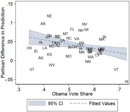
1020    |   POLITICS & POLICY / December 2012

       Moon, David. 1993. “Information Effects on the Determinants of
       Electoral Choice in Presidential Elections 1972-88.” Southeastern Political
       Review 21 (2): 365-388.
       http://onlinelibrary.wiley.com/doi/10.1111/j.1747-1346.1993.tb00368.x/abstract
       Related Media:
       FiveThirtyEight. 2008. “FiveThirtyEight: Nate Silver’s Political Calculus.”
       The New York Times.
       http://fivethirtyeight.blogs.nytimes.com/
       CNN. 2008. “Election Tracker.”
       http://www.cnn.com/ELECTION/2008/map
       Analizamos las predicciones probabilísticas individuales de los
       resultados estatales para la elección presidencial de los Estados Unidos
       en 2008. Usando una encuesta original de más de 19,000 participantes,
       encontramos que los partidistas dieron una mayor probabilidad a su
       candidato preferido, pero este sesgo se vio reducido por factores como
       la educación, sofisticación numérica, y el nivel de soporte hacia
       Obama en sus estados de origen. En conjunto, mostramos que los sesgos
       individuales se compensan y que las predicciones grupales fueron de
       gran precisión, superando a Intrade (un mercado de predicciones)
       y fivethirtyeight.com (un pronóstico basado en encuestas). La
       implicación es que los pronosticos electorales pueden ser mejorados
       al preguntar a los individuos quién piensan que ganará en lugar de
       preguntar quién quieren que gane.

    How do individuals form expectations about future political events? Are
predictions influenced by desires? Do social surroundings play a role? Guided
by these questions, this study analyzes individual forecasts of state outcomes in
the 2008 U.S. presidential election. In line with previous work, we confirm a
strong impact of preferences on expectations, known as “wishful thinking”
(WT) bias. Thus Republicans gave higher probabilities to McCain victories and
Democrats to Obama victories. At first, the presence of this bias seems to
question the epistemic value of citizen forecasts. However, we find two reasons
to be more optimistic. First, we identify several factors that reduce WT bias,
including individual sophistication and social surroundings. Second, we show
that individual biases balance out in aggregate, making the group as a whole
highly accurate.
    Although several studies have investigated electoral prediction, we draw on
an original online survey of more than 19,000 respondents, with unprecedented
variation over time and location. The survey includes respondents from all 50
states (as well as outside the United States) and covers every day in the two
months prior to the election. Further, we asked respondents their predicted
probabilities of Senators Barack Obama or John McCain winning various
states, rather than who they predicted would win nationally, providing us with
richer data than in most existing research.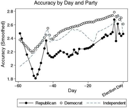
Miller et al. / CITIZEN ELECTORAL FORECASTS             |   1021

    Building on past work, we show that WT bias is reduced by education and
an original measure of numerical sophistication. In addition, we provide
the first evidence that an individual’s residence matters—respondents whose
home states gave a larger vote share to Obama had smaller WT bias and
higher accuracy. We explain this by appeal to the informational role of one’s
surroundings and social networks. The effect is robust to controlling for
other state characteristics, including campaign spending. We also investigate
how patterns of individual prediction change over time as new information
is acquired. We find that predictive accuracy improved as election day
approached, but this was almost entirely concentrated among the most
sophisticated individuals. Republicans also failed to improve their accuracy
until the election was very near, indicating an initial resistance to accept
Obama’s approaching victory.
    Guided by an interest in party evaluation and the dynamics of political
deliberation, there exists a robust literature in political science on how
preferences relate to the formulation of factual beliefs (Bartels 2002; Gerber
and Huber 2010; Mendelberg 2002; Nickerson 1998; Oswald and Grosjean
2004), information sharing (Meirowitz 2007), and the evaluation of arguments
(Kunda 1990; Taber, Cann, and Kucsova 2009). However, with the exception
of work on electoral prediction, there remains a lacuna on how expectations
form about political events. This is an unfortunate oversight, as political
scientists have several reasons to care about individual predictions of elections
and other events. Businesses and stock markets adjust their behavior based
on anticipations of future election winners (Snowberg, Wolfers, and Zitzewitz
2007). The expected closeness of races influences campaign spending
decisions (Erikson and Palfrey 2000) and voter turnout (Blais 2000). Moreover,
expectations can powerfully shape the disappointment or satisfaction
individuals experience from electoral outcomes (Classen and Dunn 2010;
Gerber and Huber 2010; Krizan, Miller, and Johar 2010; Wilson, Meyers, and
Gilbert 2003).
    Last, there exists a small cottage industry in political forecasting for
its own sake. We compare the accuracy of our survey group’s forecasts
with a prediction market (Intrade) and aggregated polling data (from
http://www.fivethirtyeight.com, hereafter 538) and find that the properly
aggregated group predictions outperform both sources at most points in time.
The implication is that forecasters can get better predictions asking individuals
who they think will win rather than who they want to win, especially more than
a month or so before election day.
    After reviewing the existing work on WT in elections, we describe
our theoretical perspective and several open questions that our study
helps to address. We then describe our survey procedure and data, followed
by the empirical results on individual accuracy and prediction. Last,
we compare the accuracy of our aggregated survey predictions with Intrade
and 538.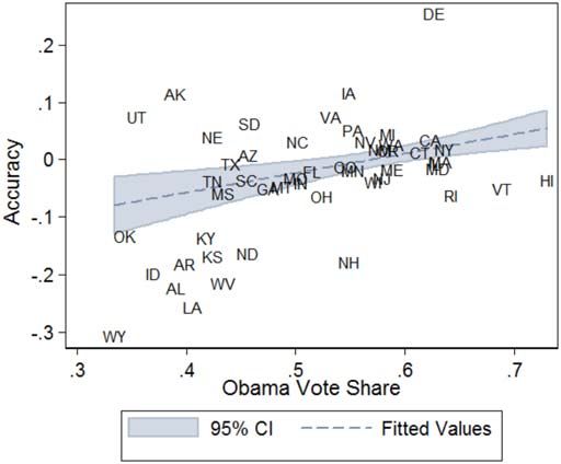
1022    |   POLITICS & POLICY / December 2012

                             Wishful Thinking in Elections

Existing Work on Wishful Thinking in Elections
    What individuals want influences what they believe. In evaluating and
constructing arguments, for instance, “[t]here is considerable evidence that
people are more likely to arrive at conclusions that they want to arrive at”
(Kunda 1990, 480). Preferences interfere with a variety of cognitive processes,
including memory, the perception of control, and information processing
(Eroglu and Croxton 2010; Kopko et al. 2011; Krizan and Windschitl 2007).
    We focus on the effect of preferences on expectations, specifically the link
between political support and electoral prediction. In numerous experiments
and surveys, subjects display WT bias, a tendency to exaggerate the likelihood
of desired events (see Krizan and Windschitl 2007 for a review). Cantril (1938)
demonstrates WT in the prediction of social and political events, such as the
outcome of the Spanish Civil War. Babad (1987) finds that 93 percent of soccer
fans expect their favored team to win, which extends to betting behavior (Babad
and Katz 1991). WT also holds among experts anticipating events, such as
physicians (Poses and Anthony 1991), politicians (Lemert 1986), and investment
managers (Olsen 1997). Further, WT bias is minimally affected by instructions
to be objective and rewards for accuracy (Babad and Katz 1991; Krizan and
Windschitl 2007).
    Electoral prediction is the best developed strand of the literature on WT. As
far back as the 1930s, Hayes (1936) showed that both voters’ and party leaders’
preferences strongly correlated with their expectations of election winners. In
the 1932 U.S. presidential election, 93 percent of Roosevelt supporters thought
he would win, whereas 73 percent of Hoover supporters predicted a Hoover win.
Using American National Election Studies data, Lewis-Beck and Skalaban
(1989) and Lewis-Beck and Tien (1999) find a consistent preference–expectation
link in each U.S. presidential election since 1956. Similar results are found
for expectations about public referenda (Granberg and Brent 1983; Lemert
1986; Rothbart 1970), as well as elections in Sweden (Granberg and Holmberg
1988; Sjöberg 2009), New Zealand (Babad, Hills, and O’Driscoll 1992; Levine
and Roberts 1991), Israel (Babad 1997; Babad and Yacobos 1993), Canada
(Johnston et al. 1992), the Netherlands (Irwin and van Holsteyn 2002), and
Great Britain (McAllister and Studlar 1991; Nadeau, Niemi, and Amato 1994).1
    Why do preferences affect expectations? Krizan and Windschitl (2007) posit
that preferences affect three distinct stages of information processing: searching
for evidence, evaluating the strength of that evidence, and formulating a final

1
 A problem in interpreting WT results is determining the direction of causation, since
bandwagoning may increase support for the expected election winner (Bartels 1985; McAllister
and Studlar 1991; Nadeau, Niemi, and Amato 1994). However, the weight of evidence indicates
that the main causal pathway between preferences and expectations is through WT bias (Johnston
et al. 1992; Krizan, Miller, and Johar 2010).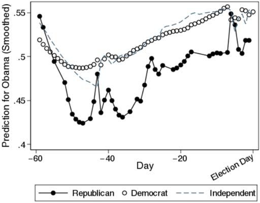
Miller et al. / CITIZEN ELECTORAL FORECASTS                       |   1023

opinion. Generally, facts confirming a desired conclusion are more available in
memory and individuals tend to be satisfied with a conclusion once they have
constructed a plausible justification for it (Kunda 1990). Moreover, projection
bias leads people to assume others have similar political opinions and attributes
as themselves (Bartels 1985; Ross, Greene, and House 1977). As a result, they
exaggerate the extent to which others favor their chosen candidate or cause.
A similar bias arises from the selective sample of associates (Gentzkow and
Shapiro 2011; Huckfeldt and Sprague 1987, 1995; Regan and Kilduff 1988)
and information sources, such as newspapers and blogs (Gentzkow and
Shapiro 2011; Redlawsk 2004). Finally, people formulate beliefs that the
“right” candidate will be chosen as a form of dissonance reduction (Regan and
Kilduff 1988).

Our Theoretical Perspective
     Although the literature has successfully established a preference–
expectation link in elections, there remain a number of open questions
concerning how WT bias and accuracy vary between individuals and across
time. We now outline our theoretical perspective and summarize our main
findings. In the following subsection, we expand on the set of open questions
that our study addresses.
     Since the literature has concentrated on establishing WT’s existence, there
has been relatively little consensus on what individual traits mitigate or amplify
WT bias (Babad, Hills, and O’Driscoll 1992; Dolan and Holbrook 2001; Eroglu
and Croxton 2010).2 We argue that two factors affect its strength: individual
sophistication and social influence.
     First, more educated and sophisticated individuals should perform better
at objectively gathering and evaluating information. The most consistent
result in the existing literature is that education reduces WT bias (Babad, Hills,
and O’Driscoll 1992; Dolan and Holbrook 2001; Granberg and Brent 1983;
Hayes 1936; Lewis-Beck and Skalaban 1989). We confirm the moderating
effect of education, concurring with Granberg and Brent (1983) that education
provides greater exposure to outside views and more experience with objectively
evaluating information.
     In addition to education, we test the effect of a novel variable (incoherence)
that proxies for a general lack of numerical sophistication. This is constructed
by asking individuals for state predictions involving complex conditionals
(such as Obama’s likelihood of winning Maine given that he wins Florida) and
calculating their numerical incoherence. An advantage of this variable is that
it is computed purely from each individual’s predictions, rather than the

2
 There is mixed evidence that WT is exacerbated by partisan intensity (Dolan and Holbrook 2001;
Granberg and Brent 1983; Levine and Roberts 1991) and reduced by knowledge (Babad 1997;
Dolan and Holbrook 2001; Sjöberg 2009). However, the act of voting is found to increase WT bias
(Frenkel and Doob 1976; Regan and Kilduff 1988).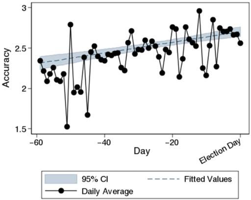
1024    |   POLITICS & POLICY / December 2012

individual’s self-report of his or her background. It is thus a more objective
indicator of numerical fallibility. We hypothesize that incoherence will predict
lower accuracy and more WT bias. Further, we expect that improvements in
forecasting accuracy over time—as more information is acquired and polling
becomes more accurate—will be concentrated among the most sophisticated
individuals. We confirm each of these hypotheses in our results.
    Second, voters’ residences and social interactions should strongly influence
electoral expectations. Because of data limitations, past work has neglected the
role of surroundings.3 This is a considerable oversight given the central role
that social networks play in dispersing political information (Borgatti and Cross
2003; Gentzkow and Shapiro 2011; Huckfeldt and Sprague 1987, 1995; Regan
and Kilduff 1988). As Huckfeldt and Sprague (1995, 124) argue, “[p]olitical
behavior may be understood in terms of individuals who are tied together by,
and located within, networks, groups, and other social formations that largely
determine their opportunities for the exchange of meaningful political
information.” Given its heterogeneous population and relatively decentralized
media environment, the United States is an ideal location for a study of
residence effects on prediction.
    To investigate social influence, we employ our large and geographically
diverse sample (including individuals from all the 50 states) to test how Obama’s
vote share in respondents’ home states influence their predictions. All things
equal, a voter in California will have more social contacts who favor Obama
than a voter in Wyoming. Although individuals tend to seek out like-minded
partners for political discussion, this selection effect is not strong enough to
erase the influence of the surrounding majority (Huckfeldt and Sprague 1995,
124-35). We consider two alternative hypotheses on how this social interaction
influences individual forecasts, one concerning the bias of electoral information
and the other the volume of information.
    A simple hypothesis is that voters from Obama-supporting states
will express more positive expectations of Obama’s chances, as they become
influenced by their associates’ optimism and surrounding signs of political
support (Uhlaner and Grofman 1986). As Granberg and Holmberg (1988, 149)
claim, voters may tell themselves, “[a]s my state goes, so goes the nation.” In this
view, WT is contagious and mutually reinforcing, just as Sunstein (2009) argues
that being surrounded by like-minded associates increases opinion extremism.
    We instead find support for a very different relationship between residence
and prediction. Stronger home-state Obama support in fact improves accuracy

3
 A partial exception is Meffert and others (2011), which finds that West Germans and Berliners
are marginally better predictors of German elections. Other work compares how individuals
predict elections in their own states versus national elections. In New Zealand, Levine and
Roberts (1991) and Babad, Hills, and O’Driscoll (1992) find that WT bias is stronger for local
results compared to national ones. However, Granberg and Brent (1983) do not find this effect
for the United States, hypothesizing that stronger bias and greater knowledge balance out.
Miller et al. / CITIZEN ELECTORAL FORECASTS | 1025
and reduces WT bias among both Democrats and Republicans. As a result,
living in a pro-Obama state makes Democrats less optimistic for Obama’s
chances across the country. This finding holds even after controlling for state
levels of education, income, media consumption, and campaign spending.
We interpret this result in terms of the volume of information exchanged.4
Given Obama’s lead throughout the survey period, Obama supporters were
more active in discussing politics and the election specifically (Fernandes et al.
2010; Winneg 2009, 95). This inevitably had informational consequences
for neighbors and social contacts, as political conversations directly increase
knowledge and encourage further media exposure, information seeking, and
discussion (Eveland and Thomson 2006; Huckfeldt and Sprague 1987, 1995;
McClurg 2006). For instance, among young adults during the 2008 U.S.
presidential campaign, “individuals’ frequency of political talk with parents,
close friends, significant others, and siblings was found to be a predictor of their
political media diet” (Rill and McKinney 2011, 64).5 Being surrounded by
Obama voters thus heightened informational exposure about the campaign and
led to more accurate electoral expectations.
Other Open Questions
We have just covered our expectations for which individual factors mitigate
WT bias and how residence affects individual predictions. We now consider four
additional open questions that our study addresses.
What Individual Factors Affect Predictive Accuracy?
As Eroglu and Croxton (2010) note, the literature on WT offers few
consistent conclusions on the factors predicting individual forecasting accuracy.
As in several previous studies (Babad 1997; Dolan and Holbrook 2001; Sjöberg
2009), we analyze the common demographic variables of sex, age, and
education. We also study the effects of two types of self-described knowledge,
party identification, and whether respondents are judging their own states.
Of greater novelty is our inclusion of incoherence and state residence.
Does Wishful Thinking Hold for Estimating Probabilities?
The measurement technique for each side of the preference–expectation link
varies across previous studies, with minimal effect on findings.6 To measure
4
As this is a novel result, we believe it should prompt further research that can confirm this pattern
and more finely trace the causal mechanisms.
5
McDevitt and Kiousis (2007) also find that classroom discussions about politics increase political
conversations among students at home.
6
To measure preferences, studies variously ask for party identification (Lemert 1986; Lewis-Beck
and Skalaban 1989; Sjöberg 2009), vote intention (Hayes 1936; Irwin and van Holsteyn 2002;
Lewis-Beck and Skalaban 1989), or candidate evaluations (Babad 1997; Babad, Hills, and
O’Driscoll 1992; Krizan, Miller, and Johar 2010).1026 | POLITICS & POLICY / December 2012
expectations, nearly all studies ask respondents to predict the election winner.7
The current study differs by asking individuals for their probability estimates
of who will win various states. Results from experimental psychology indicate
that this represents a hard case for finding a WT effect (Bar-Hillel and Budescu
1995; Krizan and Windschitl 2007; Price and Marquez 2005). In fact, our results
appear to be the first in any empirical study to find a robust WT effect for
estimating probabilities.
How Do Individual Predictions Change over Time?
A few existing studies demonstrate that electoral forecasting accuracy
improves as election day approaches (Dolan and Holbrook 2001; Krizan,
Miller, and Johar 2010; Lewis-Beck and Skalaban 1989; Lewis-Beck and Tien
1999). However, there exists little work on how other patterns of individual
prediction change. For instance, does WT bias increase or decrease closer to the
election? Do all voters increase their accuracy over time or is the effect isolated
among more sophisticated voters? Taking advantage of our large sample,
featuring responses over the two months prior to election day, we investigate
how accuracy evolved throughout the election cycle.
How Do Group Predictions Compare to Other Forecasts?
Controversy exists over the relative predictive power of expert forecasting,
polls, and prediction markets (Leigh and Wolfers 2006). An underinvestigated
method of electoral prediction is the aggregation of individual expectations.
According to the “wisdom of crowds” hypothesis (Surowiecki 2004), group
estimates should be highly accurate, outperforming even political experts.
We address two questions along these lines: first, how should individual
predictions be aggregated to maximize forecasting accuracy? Second, how does
the predictive power of these group estimates compare to prediction markets
and probability estimates derived from polls? We compare aggregated group
estimates to the predictions provided by Intrade and 538 at several points in
time. We find that a group aggregation that adjusts for the influence of prospect
theory outperforms both sources at most points in time.
The Survey and Data
The Survey Procedure
We established a website to collect probability estimates of state outcomes
in the two months prior to the 2008 U.S. presidential election, beginning
immediately after the Republican National Convention on September 4.
7
Some studies additionally ask for winning margins (Lemert 1986; Sjöberg 2009), seat totals in
parliamentary elections (Babad and Yacobos 1993), or confidence levels (Krizan, Miller, and
Johar 2010).Miller et al. / CITIZEN ELECTORAL FORECASTS | 1027
Advertisements ran on politically oriented websites to attract respondents, but
none of these websites was affiliated with a political party or candidate. Cash
prizes were offered to respondents with the highest accuracy as an incentive for
individuals to reveal their true beliefs.
Each participant was given an independent, randomly generated survey.
A given survey used a randomly chosen set of seven (out of 50) states. Each
respondent was asked 28 questions, seven of which asked for the likelihood that
a particular candidate would win each state. For instance, a respondent could
be asked, “What is the probability that Obama wins Indiana?” The remaining
21 questions involved conjunctions, disjunctions, and conditionals concerning
election outcomes in the seven states. For instance, a respondent could be asked,
“What is the probability that McCain wins Florida supposing that McCain wins
Maine?” These more complex questions allow us to measure the probabilistic
coherence of each judge. For each respondent, we randomized the seven states,
the order of simple and complex events, and the name used in each question,
McCain or Obama. Respondents provided probability estimates running from
0 to 100 percent. In total, we collected 19,215 complete sets of predictions.
As with any data collection procedure, positives and negatives come with
employing an online survey. On the positive side, we attain a size and variation
in our sample that would be infeasible using other methods. On the negative
side, there are concerns that the sample is partially self-selected and therefore
nonrepresentative, although not necessarily more so than a sample of college
students. In particular, our sample skews toward Democrats, the highly
educated, and the politically attentive, and we therefore control for these factors
in all models.
Although the sample’s composition should be kept in mind, it is unlikely
to yield significant bias in comparisons among our subjects. First, we obtain
very similar results on the size of WT bias (and its variation with education)
compared to past studies. This bolsters our confidence that the more novel
results have external validity. Second, we obtain results on WT bias by
comparing Republicans and Democrats, who in our survey are very
well-balanced on all explanatory variables. For every variable, each group’s
mean is within a half-standard-deviation of the other group’s mean. Last, the
sample’s composition does not in any way negate the use of our procedure as a
forecasting tool, as it is easily replicable in future elections.
Dependent Variables
Our analysis focuses on two dependent variables: a measure of each
respondent’s overall predictive accuracy and the respondent’s predictions for
each state. For both measures, we only incorporate the seven simple probability
estimates (i.e., none of the complex questions).
To measure individual accuracy, we use the negative log-odds of the Brier
Score (Brier 1950; Predd et al. 2008), which measures the mean squared error
of the predictions. Because the Brier Score runs strictly from 0 to 1, we use a1028 | POLITICS & POLICY / December 2012
log-odds transformation to make the measure suitable for ordinary least
squares (OLS) regression. We take the negative so that larger values correspond
to more accurate judges. Formally:
Definition 1. Let Pi be the probabilistic prediction of an election and let
Oi ∈ {0, 1} be the actual outcome. The Brier Score is defined as
1 7 0.01 + BS
BS = ∑ (Oi − Pi ) . Accuracy is defined8 as − log
2
.
7 i =1 1.01 − BS
Our second dependent variable is the probability estimate that each
individual assigned to Obama winning a state (Prediction for Obama). For the
OLS regressions, we again use a log-odds transformation.
Explanatory Variables
We collected respondents’ demographic information (gender, age, and
education9), their place of residence (among 50 states or outside the United
States), their party identification (Republican, Democrat, or independent), the
day they filled out the survey (Day), and numerical self-ratings (on a 100-point
scale) of general political knowledge and their familiarity with the election
(election knowledge). Our study employs party identification as the measure of
political preference, with the advantage that party ID is relatively stable over the
long term (Green and Palmquist 1994; Sears and Funk 1999) and thus less
susceptible to reverse causation. Of the 19,215 survey responses, 16,082 include
complete personal information, with 15,142 of these located inside the United
States. The latter total corresponds to 105,994 separate state predictions.
Finally, using all the 28 predictions per individual, we calculated
each respondents’ probabilistic incoherence as a measure of numerical
sophistication.10 Since they were asked to judge complex conditional
probabilities, individuals often supplied mathematically impossible probability
estimates. For instance, they could predict that Obama had a 50 percent
chance of winning Virginia and a 60 percent chance of winning both Virginia
and California. Incoherence measures how far a judge’s forecast departs
from a logically coherent estimate. To calculate this, we computed the
coherent forecast closest to the individual’s predictions using the Coherent
Approximation Principle proposed by Osherson and Vardi (2006).11 Incoherence
is the summed squared distance between this coherent forecast and the original
forecast. Summary statistics for all variables are displayed in Table 1.
8
We use the .01 adjustment to avoid infinite values when BS is exactly 0 or 1. Results are not
sensitive to this parameter.
9
This was measured on a nine-point scale running from no high school to a professional degree.
We include it in the regressions as an ordinal variable. Using dummies for each category returns
similar results.
10
The measure may also track how much attention the respondents were applying to the survey.
11
See Predd and others (2008) and Wang and others (2011) for past applications.Miller et al. / CITIZEN ELECTORAL FORECASTS | 1029
Table 1. Summary Statistics
Variable Mean Std.Dev. Min. Max. n
Accuracy 2.600 .926 -1.736 4.615 19,215
Prediction for Obama (log-odds) .226 2.823 -4.615 4.615 134,505
Prediction for Obama .527 .377 0 1 134,505
Obama vote share .560 .072 .334 .730 16,884
Republican .072 .258 0 1 17,763
Democrat .713 .452 0 1 17,763
Independent .215 .411 0 1 17,763
General political knowledge 81.015 15.233 0 100 19,215
Election knowledge 77.303 19.191 1 100 18,682
Incoherence .299 .403 0 3.671 19,215
Male .743 .437 0 1 18,821
Age 38.780 14.575 13 99 19,215
Education 6.865 1.804 2 9 18,659
Judging residence .127 .333 0 1 18,288
Residence education 1.256 .082 1.060 1.432 16,884
Residence income ($10,000) 3.829 .520 2.787 5.159 16,884
Residence newspapers .169 .075 .08 .40 16,884
Residence campaign spending 1.367 1.966 0 13.062 16,884
Day -15.589 17.233 -59 0 19,215
Empirical Results
We now discuss our empirical results on individual accuracy and state
forecasts. The former captures how well individuals made predictions and the
latter the direction and magnitude of predictive bias. We then consider how
these patterns changed as election day approached.
Individual Accuracy
Models 1-3 of Table 2 present the main results for individual accuracy. The
OLS models predict accuracy from the explanatory variables and four sets
of added control variables. It is necessary to account for both the day the
individual was judging and the specific states being judged. In addition, states
display different patterns across time for how easy they were to predict. The
models thus add fixed effects for each day and each of the seven states being
judged, as well as interactions of Day (as a continuous variable) and Day2 with
the state fixed effects. This sets a baseline for the difficulty of predicting each
state at each point in time (modeled as a quadratic function of Day). The
parentheses beside each coefficient show t-values based on robust standard
errors clustered by Day. We also estimated the models by dichotomizing the
predictions and testing how many of the seven states each individual predicted
correctly. All of the results from Table 2 hold.
The first result worth highlighting is the effect of party identification.
Democrats performed better than independents, and Republicans performedTable 2. OLS Regressions of Accuracy and Prediction for Obama
1030
|
Accuracy Prediction for Obama (log-odds)
(1) (2) (3) (4) (5)
Obama vote share .345*** (4.11) .406** (3.12) -.076 (-1.02)
Republican ¥ Obama vote share .808** (3.10) .595* (2.11)
Democrat ¥ Obama vote share .391** (3.38) -.213* (-2.45)
Independent ¥ Obama vote share .033 (.23) .102 (.62)
Republican -.199*** (-6.74) -.199*** (6.60) -.626*** (-3.77) -.265*** (-10.01) -.535** (-2.88)
Democrat .067*** (4.04) .067*** (4.02) -.132 (-1.29) .041** (3.02) .216* (2.06)
General political knowledge .002** (3.05) .002** (3.05) .002** (3.04) .001 (1.46) .001 (1.46)
Election knowledge .010*** (26.00) .010*** (26.04) .010*** (25.89) -.001** (-2.69) -.001** (-2.70)
Incoherence -.177*** (-6.94) -.177*** (-6.96) -.176*** (-6.85) .080*** (3.85) .080*** (3.87)
Male .182*** (17.83) .182*** (17.80) .181*** (17.69) -.065*** (-4.97) -.065*** (-4.97)
Age -.007*** (-10.41) -.007*** (-10.56) -.007*** (-10.41) .002*** (5.84) .002*** (5.85)
Education .008 (1.62) .008 (1.63) .008 (1.61) -.018*** (-5.42) -.018*** (-5.41)
Judging residence -.027 (-1.39) -.027 (-1.39) -.027 (-1.42)
Residence education -.053 (-.37)
Residence income -.11 (-.54)
POLITICS & POLICY / December 2012
Residence newspapers .156 (1.80)
Residence campaign spending .002 (.69)
Day fixed effects (FEs) Y Y Y Y Y
Judged State FEs Y Y Y Y Y
J. State FEs ¥ Day Y Y Y Y Y
J. State FEs ¥ Day2 Y Y Y Y Y
n 15,142 15,142 15,142 105,994 105,994
Adjusted R2 .332 .332 .332 .725 .725
BIC 34,690.5 34,695.6 34,694.5 385,413.3 385,422.3
Notes: Models 1-3 predict individual accuracy. t-Statistics (based on robust standard errors clustered by Day) are shown in parentheses. Models 4-5
estimate the Prediction for Obama (log-odds) given for seven states per individual. t-Statistics (based on robust standard errors clustered by individual)
are shown in parentheses. * p < .05; ** p < .01; *** p < .001.Miller et al. / CITIZEN ELECTORAL FORECASTS | 1031
Figure 1.
Accuracy by Residence
Notes: Figure 1 shows state residence fixed effects for accuracy against Obama vote share
after accounting for the standard controls. Non-U.S. respondents are the reference
group. The dotted line is a linear fit weighted by the state’s number of respondents.
Individuals from Obama-supporting states are significantly more accurate (n = 16,884).
considerably worse. In fact, the difference between Republicans and
independents is about three times the difference between Democrats and
independents. As we explore below, WT is the main cause—Democrats were
optimistic about Obama’s chances, and the election ended up being very
successful for him.
State Residence. Consistent with our expectation that social surroundings can
matter, model 1 finds that respondents from states with a higher Obama vote
share (his portion of the two-party vote) were significantly more accurate.
Non-U.S. respondents are dropped from this model’s sample, but on average
they were even more accurate than individuals in states won by Obama. A
more detailed picture is provided by Figure 1. State fixed effects for accuracy
are plotted against the state’s Obama vote share. The dotted line displays
a weighted linear fit of the relationship and the shaded area the 95 percent
confidence interval.12
12
The linear fit weights by the number of respondents in each state. This is equivalent to an
individual-level regression using standard errors clustered by state.1032 | POLITICS & POLICY / December 2012
Obama vote share is correlated with several other state characteristics that
may also increase accuracy. To see if the effect is robust, model 2 controls for
levels of education, income, newspaper consumption, and campaign spending in
respondents’ home states. Residence education is the summed fractions of state
residents aged 25 or older with high school, bachelor, and advanced degrees.
Residence income is per capita income (in $10,000). Residence newspapers is the
per capita circulation of daily newspapers. All three are 2008 figures taken from
the U.S. Census Bureau (2011). Residence campaign spending is summed per
capita ad spending (in U.S. dollars) from the two presidential campaigns.13 The
first three are positively correlated with Obama support, but the coefficient on
Obama vote share only increases in magnitude in model 2.
Finally, model 3 separates out the effect of Obama vote share by party
identification. Previewing results below, Obama vote share improves the
accuracy of Republicans and Democrats, but not independents. Moreover, the
effect is strongest for Republicans.
Other Controls. Results for the remaining control variables are highly
consistent across models. Higher values of self-described knowledge improve
accuracy, with the effect of election knowledge greater in magnitude than general
political knowledge. Thus, respondents were good judges of their own predictive
ability. As expected, the two measures of sophistication—higher education and
lower incoherence—predict greater accuracy, although education’s effect is
insignificant. Surprisingly, individuals are less accurate at judging their home
states, although not significantly.14 Finally, men and younger individuals are
found to be more accurate.
Individual Predictions
Models 4-5 in Table 2 and the five models in Table 3 directly test for the
presence and magnitude of WT bias by looking at individual predictions for
Obama. We use the same set of controls as for accuracy and cluster standard
errors by individual survey to account for differences across individuals.
As evidence for WT bias, model 4 shows that the coefficient on Republican
is negative and the coefficient on Democrat is positive. That is, party members
rated their candidate’s likelihood of winning higher. Figure 2 shows the
differences in mean estimates provided by Democrats and Republicans
compared with independents, averaged across the 50 states being judged and
calculated with and without the control variables. On average, Democrats
overestimated Obama’s chances in each state by .6 percent relative to
13
These data are available from CNN (2008).
14
In other results, we source this effect mostly to Democrats significantly overestimating Obama’s
chances in their home states, perhaps being swept away by the highly visible enthusiasm of the
Obama campaign. These results are available from the authors on request.Miller et al. / CITIZEN ELECTORAL FORECASTS | 1033
Figure 2.
Difference of Mean Predictions
Notes: Figure 2 shows the difference in mean prediction for Obama between Democrats
and independents and between Republicans and independents. The circle points
represent the simple difference of means. The square points show the difference of
means after accounting for the standard control variables. The bars show 95 percent
confidence intervals. All party identifiers display wishful thinking bias, but the effect is
stronger for Republicans (n = 16,489; 15,099).
independents, whereas Republicans underestimated his chances by 3.1 percent.
Again, we speculate that the larger bias among Republicans stems from
Obama’s ascendancy during the period.
State Residence. Being surrounded by Democrats does not have the same
straightforward effect as personal party identification. As seen in model 4, a
higher Obama vote share actually leads to slightly lower expectations for Obama.
Model 5 shows what is happening—higher Obama vote share leads Republicans
to raise their expectations for Obama but has the opposite effect on Democrats.
In other words, Obama vote share reduces WT bias.
Size of Wishful Thinking Bias. Table 3 further investigates variation in WT
bias. The sample includes only Republicans and Democrats, thus the coefficient
on Democrat measures the difference in their average predictions for Obama, an
appropriate measure of WT bias. In each regression, Democrat is further1034
|
Table 3. OLS Regressions of Size of Wishful Thinking Bias
Prediction for Obama (log-odds)
(1) (2) (3) (4) (5)
Democrat ¥ education -.052*** (-3.43) -.047*** (-3.35)
Democrat ¥ incoherence .383*** (4.06) .338*** (3.82)
Democrat ¥ general political knowledge .007*** (4.14) .008*** (4.31)
Democrat ¥ Obama vote share -.792** (-2.68) -.596* (-2.08)
Democrat .644*** (5.99) .182*** (6.02) -.274* (-1.96) .742*** (4.39) .207 (.97)
Obama vote share -.127 (-1.53) -.139 (-1.68) -.128 (-1.54) .581* (2.06) .397 (1.45)
General political knowledge .001 (1.06) .001 (1.23) -.006*** (-3.46) .001 (1.06) -.006*** (-3.59)
Election knowledge -.001** (-3.02) -.001** (-3.06) -.001** (-2.99) -.001** (-3.01) -.001** (-3.04)
Incoherence .065** (2.91) -.284** (-3.10) .068** (3.01) .066** (2.94) -.239** (-2.79)
Male -.064*** (-4.44) -.062*** (-4.32) -.064*** (-4.48) -.063*** (-4.36) -.066*** (-4.57)
Age .003*** (5.89) .003*** (5.82) .003*** (5.71) .003*** (5.86) .003*** (5.68)
Education .026 (1.77) -.020*** (-5.45) -.020*** (-5.26) -.020*** (-5.34) .022 (1.62)
Day fixed effects (FE) Y Y Y Y Y
POLITICS & POLICY / December 2012
Judged State FEs Y Y Y Y Y
J. State FEs ¥ day Y Y Y Y Y
J. State FEs ¥ day2 Y Y Y Y Y
n 83,895 83,895 83,895 83,895 83,895
Adjusted R2 .729 .729 .729 .729 .729
BIC 304,667.0 304,626.1 304,664.7 304,686.5 304,595.3
Notes: The models estimate the Prediction for Obama (log-odds) given for seven states per individual, using a sample of party identifiers. The models
investigate what reduces or exacerbates wishful thinking bias. t-Statistics (based on robust standard errors clustered by individual) are shown in
parentheses. We find that education and Obama vote share reduce wishful thinking bias, whereas incoherence and self-rated knowledge increase it.
* p < .05; ** p < .01; *** p < .001.Miller et al. / CITIZEN ELECTORAL FORECASTS | 1035
interacted with another variable, thereby testing how WT’s magnitude
fluctuates. Since the direct impact of Democrat is positive, a negative coefficient
on the interaction term indicates a reduction of WT bias.
Models 1 and 2 confirm our expectations on individual sophistication.
Education reduces WT bias, the most consistent result in the previous literature.
By contrast, incoherence exacerbates it—less numerically sophisticated
respondents were especially influenced by party preference. Surprisingly, model
3 shows that self-rated knowledge increase WT bias.15 We hypothesize that this
is because knowledge proxies for interest in the campaign and by extension
partisan intensity.16
Model 4 confirms that Obama vote share reduces WT bias, supporting
our argument that social surroundings and information exchange can reduce
bias. The effect is substantial—the estimation implies that a move from
Wyoming to Hawaii reduces WT bias more than changing from a high
school education to a doctorate. As above, this finding is robust to including
interaction terms with the levels of education, income, newspaper
consumption, and campaign spending in respondents’ home states. Last,
model 5 controls for all four interaction terms simultaneously. Each of the
effects remains significant.
Figure 3 displays state-by-state results on WT bias. Using a sample of party
identifiers and accounting for the standard controls, the figure shows the
difference in the average predictions of Republicans and Democrats plotted
against Obama vote share. The dotted line displays a weighted linear fit of the
relationship and the shaded area the 95 percent confidence interval.17 WT bias is
positive in all but four states, but greater Obama support is associated with a
smaller WT effect among the state’s residents.
Variation by Day
Clocking from 59 days prior to the election up until the morning of election
day, our data provide a rich picture of how individual predictions change as
time passes and new information is acquired. Figure 4 shows the average
accuracy for each day in the sample, combined with a linear fit. Despite some
noise, individuals became significantly better at prediction as time progressed.
We now investigate how this improvement is divided across individuals.
We categorize respondents into three equally sized groups according to their
level of incoherence. Figure 5 shows accuracy averaged by day and incoherence
15
The result for election knowledge is substantively identical.
16
Knowledge increases WT bias but still improves accuracy because it reduces the variance of
predictions. Since accuracy is calculated from the squared error of predictions, it is a function of
both squared bias and variance.
17
The linear fit weights by the number of respondents in each state. This is equivalent to an
individual-level regression using standard errors clustered by state.1036 | POLITICS & POLICY / December 2012
Figure 3.
Wishful Thinking Effect by Residence
Notes: Figure 3 shows wishful thinking bias (the difference between Democrats and
Republicans in average prediction for Obama) in each state plotted against Obama vote
share. The difference is calculated after accounting for the standard control variables,
with the exception of the party dummies. The dotted line is a linear fit weighted by the
state’s number of respondents (n = 16,884).
level. For ease of interpretation, accuracy is smoothed using a loess curve
with a bandwidth of .1. The least incoherent group improved markedly and
consistently over time. In contrast, the bottom two-thirds of respondents
improved their average accuracy marginally, if at all. Hence, the utilization of
information as the campaign season progressed was highly concentrated among
more sophisticated observers.
Dividing accuracy by day and party identification in Figure 6, we find
that Democrats and independents were consistently more accurate than
Republicans. Further, Democrats improved steadily over time, whereas
Republicans were no more accurate 20 days prior to election day than 59 days
prior. However, Republicans rapidly caught up to Democrats about two weeks
prior to election day, perhaps indicating an unwillingness to acknowledge
Obama’s advantage until his national victory was all but certain.
Finally, Figure 7 shows the smoothed average of prediction for Obama by
day and party identification. For clarity, prediction for Obama is the probabilityMiller et al. / CITIZEN ELECTORAL FORECASTS | 1037
Figure 4.
Accuracy by Day
Notes: Figure 4 shows average accuracy by day, along with a linear fit weighted by
sample size. The period begins immediately after the Republican National Convention
on September 4, 2008. Respondents steadily improved their accuracy over time
(n = 19,215).
estimate rather than the log-odds transform. The difference between Democrats
and Republicans tracks the strength of WT bias. Except for very early and very
late in the period, WT bias is fairly consistent across time and hovers around
4-5 percent.
Testing the “Wisdom of Crowds”
Macroeconomic voting models, polls, and prediction markets remain the
most common methods of forecasting elections. Political scientists have
developed forecasting models using factors like incumbency, macroeconomic
variables (Abramowitz 2004; Fair 2002), and battle deaths (Hibbs 2008).18 Polls
are of course the most common predictive tool among the public and the media
(Irwin and van Holsteyn 2002), with their accuracy increased by suitable
aggregation (Jackman 2005; Lock and Gelman 2010). In prediction markets,
individuals purchase shares that pay off depending on the outcomes of specific
18
See Jones (2008) and Walker (2008) for reviews.1038 | POLITICS & POLICY / December 2012
Figure 5.
Accuracy by Day and Incoherence Level
Notes: Figure 5 shows average accuracy by day and level of incoherence (split
into three equally sized groups). The lines are smoothed using a loess curve with a
bandwidth of .1. The improvement in Accuracy over time is heavily concentrated
among the least incoherent (most numerically sophisticated) respondents
(n = 19,215).
elections. The share prices can thus be interpreted as expected likelihoods of the
electoral outcomes, prompting a great deal of interest in the markets’ predictive
powers (Ray 2006; Surowiecki 2004; Tziralis and Tatsiopoulos 2007; Wolfers
and Zitzewitz 2004). There is disagreement over the relative accuracy of
forecasting models, polls, and prediction markets, with Leigh and Wolfers
(2006) giving the edge to prediction markets and Jones (2008) and Erikson and
Wlezien (2008) finding polls to be the most accurate.
We test an alternative forecasting method supported by the “wisdom
of crowds” hypothesis that group predictions should be highly accurate
(Surowiecki 2004). We compare the accuracy of group estimates derived from
our sample with probability estimates provided by 538 (a poll aggregator run by
Nate Silver) and Intrade (a prediction market), both of which were highly
successful at predicting the 2008 election. These provide the best points of
comparison as both sites predicted state outcomes at several points in time,
whereas forecasts by political scientists generally focus on a single national
estimate. Lewis-Beck and Tien (1999), Jones (2008), and Sjöberg (2009) are the
only studies we know of that compare electoral forecasting accuracy betweenMiller et al. / CITIZEN ELECTORAL FORECASTS | 1039
Figure 6.
Accuracy by Day and Party
Notes: Figure 6 shows average accuracy by day and party identification. The lines are
smoothed using a loess curve with a bandwidth of .1. Republicans were least accurate
throughout but partially caught up immediately before election day (n = 17,763).
individual surveys and polls, whereas no previous study has compared surveys
and prediction markets.19
As a first indication of group accuracy, Figure 8 shows how the median
prediction for each state relates to the outcome (in terms of Obama’s vote share
in the state being judged). We expect an S-curve relationship, since even small
vote margins translate into high likelihoods that a candidate will win a majority.
This is indeed what we see in Figure 8. Despite including responses up to two
months before the election, the median prediction was incorrect only for
Indiana, although the median prediction for Missouri was exactly .5. Both
Intrade and 538 predicted one state incorrectly immediately before the election.
For a fuller comparison with Intrade and 538, we break down the 60 days
prior to the election into nine weeks. For Intrade, we compute the weekly
mean of each state-level contract’s bid and ask prices and interpret this mean
as the market’s predicted probability. For 538, we have four predictions at
19
In the U.S. context, Lewis-Beck and Tien (1999) and Jones (2008) give a slight edge to polls over
surveys of citizens and experts, respectively. In contrast, for the 2006 Swedish parliamentary
election, Sjöberg (2009) finds that median predictions from a public survey outperformed polls.
Lewis-Beck and Stegmaier (2011) and Murr (2011) show that aggregated expectations accurately
predict British elections but do not compare this to any other method.1040 | POLITICS & POLICY / December 2012
Figure 7.
Prediction for Obama by Day and Party
Notes: Figure 7 shows average prediction for Obama by day and party identification.
The lines are smoothed using a loess curve with a bandwidth of .1. Although wishful
thinking bias is evident throughout the two months (especially for Republicans), it was
smaller in magnitude early and late in the period (n = 17,763).
two-week intervals. We compare these predictions to weekly aggregations of
our respondents’ forecasts, using three methods: the mean, the median, and a
sharpened median that accounts for the influence of prospect theory. For the
latter, we use a transformation technique that corrects for the individual
tendency to overweight small probabilities and underweight large probabilities
(Kahneman and Tversky 1979; Tversky and Kahneman 1992). Our respondents
tended to assign small but unrealistically high probabilities to extremely
unlikely events like Obama winning Wyoming. We apply a sigmoid
transformation so that the adjusted probability is:
1
f ( Pi ) =
1 + e B (0.5− Pi )
where Pi is the original prediction and B is a tuning parameter we set at 10.20
This shifts small probabilities toward 0 and large probabilities toward 1. We
then take the median of these adjusted probabilities.
20
This is a standard value that was not chosen to maximize accuracy. Different values of B give
very similar results.Miller et al. / CITIZEN ELECTORAL FORECASTS | 1041
Figure 8.
Median Predictions for Each State
Notes: For each state, Figure 8 shows the median prediction for Obama against the
state’s outcome in Obama vote share. Note that Obama vote share now refers to the state
being judged, not the respondent’s residence. We find the expected S-shaped curve
relating vote share and winning probability (n = 19,215).
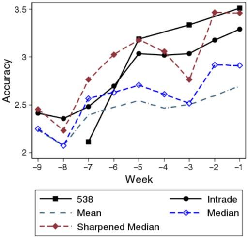
Figure 9 compares the accuracy of the five prediction methods over time.
First, the sharpened median outperforms the simple median, which in turn
outperforms the mean of our respondents.21 Second, the sharpened median is
more accurate than Intrade in seven of nine weeks. Third, 538 is highly accurate
close to election day, but is the worst of the five methods seven weeks prior.22 In
comparison, the sharpened median is virtually identical in accuracy immediately
before the election and superior more than five weeks before the election. More
complex aggregation procedures that weight judges by their coherence produce
even more accurate results. However, we wish to emphasize that even simple
aggregations of individual predictions can outperform the most sophisticated
forecasting methods, especially early in the election period.
Conclusion
This study analyzed individuals’ state-level predictions for the 2008
U.S. presidential election. We found that respondents who were Democratic,
21
As Surowiecki (2004) explains, the median’s superior performance compared to the mean
follows from the logic of the Condorcet Jury Theorem.
22
This is consistent with past findings that polls (the basis of 538’s forecasts) are highly variable
early in the election period but rapidly become more accurate closer to the election (Gelman and
King 1993; Wlezien and Erikson 2002).1042 | POLITICS & POLICY / December 2012
Figure 9.
Accuracy of Group Predictions versus Intrade and 538
Notes: Figure 9 compares the accuracy of our group survey predictions with Intrade
and 538 over time. A sharpened median of our respondents (which accounts for
prospect theory bias) outperforms Intrade in seven of nine weeks. It also outperforms
538 early in the election season and is nearly identical to 538 close to election day
(n = 19,215).
younger, more numerically sophisticated, and gave themselves higher
self-ratings of political knowledge were more accurate. We also uncovered
strong support for WT bias in expectations, which was reduced by higher
education and numerical sophistication. In addition, the vote share for Obama
in respondents’ home states predicted higher accuracy and lower WT bias.
The implication is that people are often fallible in allowing their desires to
seep into their predictions, but this bias can be ameliorated by both individual
education and greater information exchange. These results encourage further
work on how political preferences relate to the formation of expectations.
Future research can investigate the full range of personal characteristics and
social influences that improve accuracy and mitigate or exacerbate WT.
Finally, we compared the forecasting accuracy of our survey group with
predictions derived from polling and a prediction market. When estimates were
sharpened to account for prospect theory, the group median was the most
accurate at most points in time. This confirms that groups can be highlyMiller et al. / CITIZEN ELECTORAL FORECASTS | 1043
accurate even in the presence of individual bias, an optimistic sign for the
epistemic capacity of democratic polities and markets to aggregate information
(Surowiecki 2004). If further verified in future elections, the approach of
aggregating individual expectations may greatly improve the accuracy of
electoral forecasting for news organizations, campaigns, and political scientists.
Although we relied on an online survey to maximize our sample size, a
controlled sample balanced by party and location may be even more accurate.
Our results also show improved accuracy after accounting for WT, respondent
location, and numerical sophistication. It remains an open question whether an
optimal aggregation technique can consistently outperform other forecasting
methods at all points in time.
About the Authors
Michael K. Miller is a lecturer in the School of Politics & International
Relations at Australian National University.
Guanchun Wang is a cofounder of jinwankansha.com, a social movie
recommendation site, and received his PhD in Electrical Engineering from
Princeton University.
Sanjeev R. Kulkarni is a professor in the Department of Electrical
Engineering at Princeton University.
H. Vincent Poor is the Michael Henry Strater University Professor of
Electrical Engineering and Dean of the School of Engineering and Applied
Science at Princeton University.
Daniel N. Osherson is a professor in the Department of Psychology at
Princeton University.
References
ABRAMOWITZ, ALAN I. 2004. “When Good Forecasts Go Bad: The
Time-for-Change Model and the 2004 Presidential Election.” Political Science
and Politics 37 (4): 745-746. Accessed on September 15, 2012. Available online
at http://www.apsanet.org/imgtest/GoodForecastsGoBad-Abramowitz.pdf
BABAD, ELISHA. 1987. “Wishful Thinking and Objectivity among Sports
Fans.” Social Behaviour 2 (4): 231-240. Accessed on September 15, 2012.
Available online at http://psycnet.apa.org/psycinfo/1989-24476-001
___. 1997. “Wishful Thinking among Voters: Motivational and Cognitive
Influences.” International Journal of Public Opinion Research 9 (2): 105-125.
Accessed on September 15, 2012. Available online at http://ijpor.oxford
journals.org/content/9/2/105.shortYou can also read