Characterizing severe weather potential in synoptically weakly forced thunderstorm environments
←
→
Page content transcription
If your browser does not render page correctly, please read the page content below
Nat. Hazards Earth Syst. Sci., 18, 1261–1277, 2018
https://doi.org/10.5194/nhess-18-1261-2018
© Author(s) 2018. This work is distributed under
the Creative Commons Attribution 4.0 License.

Characterizing severe weather potential in synoptically weakly
forced thunderstorm environments
Paul W. Miller and Thomas L. Mote
Department of Geography, University of Georgia, Athens, GA 30602, USA

Correspondence: Paul W. Miller (paul.miller@uga.edu)

Received: 9 August 2017 – Discussion started: 9 October 2017
Revised: 30 January 2018 – Accepted: 2 April 2018 – Published: 27 April 2018

Abstract. Weakly forced thunderstorms (WFTs), short-lived         1   Introduction
convection forming in synoptically quiescent regimes, are
a contemporary forecasting challenge. The convective en-          Weakly forced thunderstorms (WFTs), convection forming
vironments that support severe WFTs are often similar to          in synoptically benign, weakly sheared environments, are
those that yield only non-severe WFTs and, additionally,          a dual forecasting challenge. Not only is the exact loca-
only a small proportion of individual WFTs will ultimately        tion and time of convective initiation difficult to predict,
produce severe weather. The purpose of this study is to bet-      but, once present, the successful differentiation of severe
ter characterize the relative severe weather potential in these   WFTs from their benign counterparts is equally demanding.
settings as a function of the convective environment. Thirty-     Consequently, severe weather warnings issued on WFTs in
one near-storm convective parameters for > 200 000 WFTs           the US are less accurate than more organized storm modes,
in the Southeastern United States are calculated from a high-     such as squall lines and supercells (Guillot et al., 2008).
resolution numerical forecasting model, the Rapid Refresh         American operational meteorologists have coined these se-
(RAP). For each parameter, the relative odds of WFT days          vere WFTs “pulse thunderstorms” because the surge of the
with at least one severe weather event is assessed along          updraft that produces the severe weather occurs in a brief
a moving threshold. Parameters (and the values of them) that      “pulse” (Miller and Mote, 2017). The United States Na-
reliably separate severe-weather-supporting from non-severe       tional Weather Service defines “severe weather” as any of
WFT days are highlighted.                                         the following: winds ≥ 26 m s−1 , hail ≥ 2.54 cm in diameter,
   Only two convective parameters, vertical totals (VTs)          or a tornado.
and total totals (TTs), appreciably differentiate severe-wind-       Environments thought to support pulse thunderstorms are
supporting and severe-hail-supporting days from non-severe        typically characterized by weak vertical wind shear and
WFT days. When VTs exceeded values between 24.6 and               strong convective available potential energy (CAPE). How-
25.1 ◦ C or TTs between 46.5 and 47.3 ◦ C, odds of severe-        ever, not all weak-shear, high-CAPE environments facili-
wind days were roughly 5× greater. Meanwhile, odds of             tate pulse thunderstorms, nor are all pulse thunderstorms
severe-hail days became roughly 10× greater when VTs              confined to environments with the weakest shear and/or
exceeded 24.4–26.0 ◦ C or TTs exceeded 46.3–49.2 ◦ C. The         strongest instability. The result is a low signal-to-noise ra-
stronger performance of VT and TT is partly attributed to the     tio (SNR) which obstructs the reliable discernment of pulse-
more accurate representation of these parameters in the nu-       supporting environments. The SNR is a common discussion
merical model. Under-reporting of severe weather and model        point in climate variability research, where it often describes
error are posited to exacerbate the forecasting challenge by      the relative magnitudes of a climate change trend (i.e., the
obscuring the subtle convective environmental differences         signal) vs. interannual variability (i.e., the noise) (e.g., Ham-
enhancing storm severity.                                         lington et al., 2010; Sutton and Hodson, 2007; Trenberth,
                                                                  1984). In our context, the “signal” refers to the true differ-
                                                                  ence between the large-scale convective environments that
                                                                  support severe weather and those that do not. Meanwhile,

Published by Copernicus Publications on behalf of the European Geosciences Union.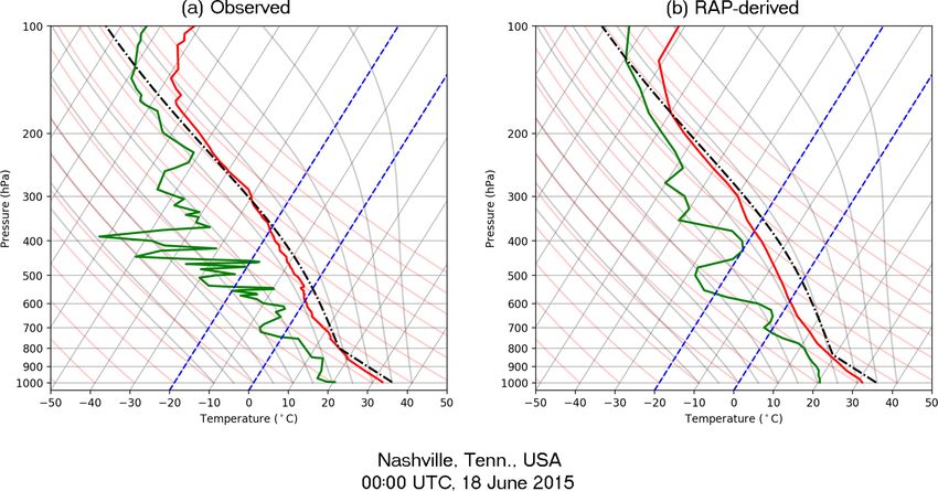
1262                                                     P. W. Miller and T. L. Mote: Characterizing severe weather potential

the “noise” represents the many processes than might cause              However, the comparative utility of these environmental
storms to produce (not produce) severe weather in an envi-           parameters within weakly forced regimes is unclear, particu-
ronment where it was not expected (expected). Cell inter-            larly when they are tested with a realistic proportion of severe
actions, stabilization from prior convection, surface conver-        storms. Many of the results above were obtained by analyz-
gence, locally enhanced shear, and model error, for example,         ing relatively small datasets, and they have not been tested
can act as noise in the operational setting.                         against each other in a weakly forced environment. There-
   Prior research directed at pulse thunderstorms is limited,        fore, this study seeks to compare the relative skill of con-
and work has not typically included a representative pro-            vective parameters using a large WFT dataset to determine
portion of non-severe WFTs in their samples (Atkins and              which are most appropriate for detecting environments sup-
Wakimoto, 1991; Cerniglia and Snyder, 2002). If the sam-             portive of pulse-thunderstorm-related severe weather.
ple contains too many pulse thunderstorms, the SNR may be
artificially bolstered, results overstated, and the potential re-
liability in an operational setting diminished. For instance,        2     Data and methods
in a meta-analysis of studies pertaining to new lightning-
based storm warning techniques, Murphy (2017) found that             2.1    WFT selection and environmental characterization
the studies’ reported false alarms ratios were directly propor-
tional to the fraction of non-severe storms contained in the         This study uses the 15-year WFT dataset developed by Miller
sample. Samples that included a realistic ratio of severe to         and Mote (2017) for the Southeastern US (Fig. 1). Their de-
non-severe storms demonstrated the weakest skill scores.             tection method first identifies thunderstorms as regions of
   Most research considering pulse thunderstorms in the              spatiotemporally contiguous composite reflectivities meeting
Southeastern US has typically focused on one of its primary          or exceeding 40 dBZ using connected neighborhoods label-
severe weather mechanisms: the wet microburst. Severe wet            ing. Each thunderstorm is then assigned five morphological
microbursts generally occur in atmospheres characterized by          attributes describing its shape, duration, intensity, etc., and all
a deep moist layer extending from the surface to 4–5 km a.g.l.       thunderstorms are clustered into 10 morphologically similar
(Johns and Doswell, 1992). Above the moist layer lies a mid-         groups using Ward’s clustering (Ward, 1963). The compos-
level dry layer with lower equivalent potential temperature          ite convective environments associated with each morpho-
values (θe ). In wet microburst environments, the difference         logical group were characterized using radiosonde observa-
between the maximum θe observed just above the surface               tions from three launch sites in the Southeastern US. WFTs
and the minimum θe aloft exceeded 20 K, whereas non-                 were designated as the subset of morphological groups with
microburst-producing thunderstorm days had differences less          small, short-lived, diurnally driven thunderstorms that also
than 13 K (Atkins and Wakimoto, 1991; Roberts and Wilson,            formed in weak-shear, strong-instability composite environ-
1989; Stewart, 1991; Wheeler and Spratt, 1995). However,             ments. Table 1 provides the composite kinematic and ther-
Atkins and Wakimoto (1991) examined only 14 microburst               modynamic environmental characteristics for the 10 morpho-
days vs. 3 non-microburst days. Adding to the uncertainty,           logical groups from Miller and Mote (2017). The WFTs are
James and Markowski (2010) challenged the role of mid-               spatially referenced according to their first-detection loca-
level dry air in severe weather production. The results of their     tion, the centroid of the composite reflectivities constituting
cloud-scale modeling experiment indicated that, for all but          the first appearance on radar. The storms were then paired
the highest instabilities tested, drier mid-level air did not cor-   with severe weather reports from the publication Storm Data,
respond to increased downdraft and cold pool intensity.              a storm event database maintained by the United States Na-
   Building on these findings, several severe weather fore-          tional Centers for Environmental Information, to differenti-
casting parameters have been developed to distill the atmo-          ate benign WFTs from pulse thunderstorms. The entire 15-
sphere’s vertical thermodynamic profile into a single value          year dataset contains 885 496 WFTs including 5316 pulse
representing the damaging wind potential. McCann (1994)              thunderstorms.
developed a microburst-predicting “wind index” (WINDEX)                 Meanwhile, the thermodynamic and kinematic environ-
to be used in the forecasting of wet downburst potential.            ment of each WFT was characterized using the 0 h Rapid
However, although WINDEX performed well when tested                  Refresh (RAP) analysis. The RAP, implemented on 9 May
in known microburst environments, no null cases were pre-            2012, is a 13 km non-hydrostatic weather model initialized
sented (McCann, 1994). Additional severe-wind potential in-          hourly for the purpose of near-term mesoscale forecast-
dices include the wind damage parameter and the microburst           ing which is operated by the United States National Cen-
index described by the United States Storm Prediction Center         ters for Environmental Prediction. The RAP uses the Na-
(SPC; http://www.spc.noaa.gov/exper/soundings/help/index.            tional Oceanic and Atmospheric Administration (NOAA)
html, last access: 20 April 2018). Tools such as TTs, K-             Gridpoint Statistical Interpolation (GSI) system to assimi-
index, and the Severe WEAther Threat (SWEAT) index,                  late radar reflectivity, lightning flashes (added in version 3),
among others, are also commonly used to forecast convec-             radiosonde observations, GOES cloud analysis, wind pro-
tive potential as well as the severity of thunderstorms.             filer data, surface station observations, etc. Lateral bound-

Nat. Hazards Earth Syst. Sci., 18, 1261–1277, 2018                            www.nat-hazards-earth-syst-sci.net/18/1261/2018/
P. W. Miller and T. L. Mote: Characterizing severe weather potential 1263
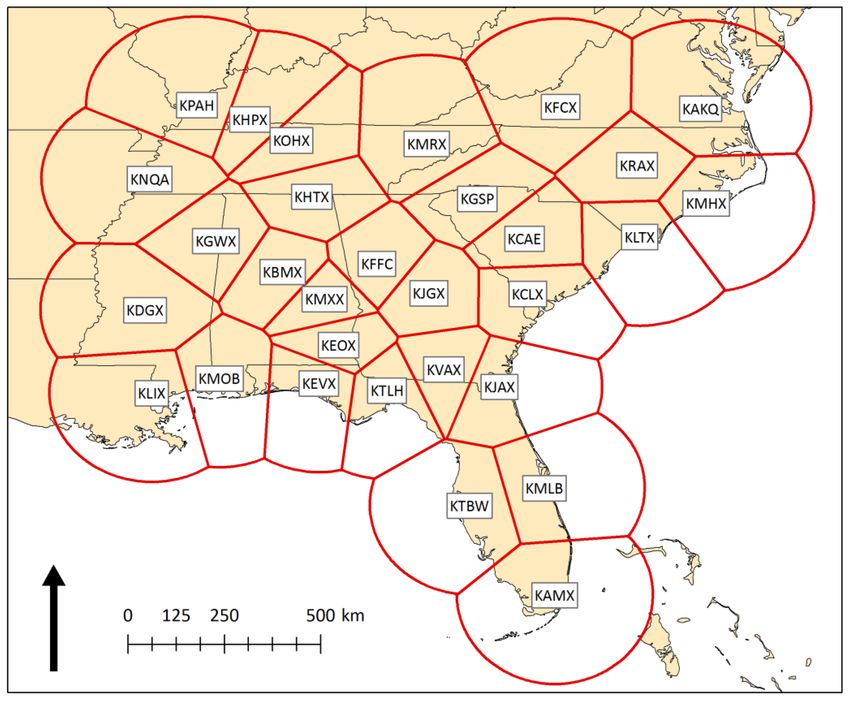
Figure 1. WSR-88D sites contributing to the Miller and Mote (2017) WFT climatology.
Table 1. Kinematic and thermodynamic parameters of 12:00 UTC composite soundings from Atlanta, GA, USA, for each radar-identified
morphological type in Miller and Mote (2017). Morphological types classified as WFTs are bolded. All kinematic values are shown in m s−1 ,
whereas the units of the thermodynamic parameters are provided in the table. Explanations for the variable abbreviations can be found in
Table 2 and Appendix A.
Type 0–6 km_SHR 0–8 km_SHR 0–12 km max wind 0–12 km mean wind ThE_LOW MLCAPE Forecast SBCAPE
(K) (J kg−1 ) (J kg−1 )
1 4.3 5.1 7.2 3.0 343.0 562 1585
2 4.3 5.1 8.8 3.6 341.9 365 1214
3 4.7 6.2 9.4 3.7 340.5 289 1176
4 4.3 5.7 8.3 3.7 341.1 357 1121
5 3.2 5.1 9.6 3.2 341.7 283 1006
6 6 7.7 11.6 5.0 339.0 211 973
7 8.2 10.8 16.5 6.1 336.6 66 723
8 4.9 7.7 13.6 3.1 336.0 24 558
9 5.4 8.7 15.4 3.0 330.6 0 32
10 7.9 9.8 13.5 5.8 334.5 0 391
ary conditions are provided by the Global Forecast System vs. non-supercellular and tornadic vs. non-tornadic thunder-
(GFS). Additional information regarding the RAP assimila- storms (Thompson et al., 2007, 2014).
tion system and model physics can be found in Benjamin For the grid cell containing each WFT’s first-detection
et al. (2016). The model has output available at 37 vertical location, a RAP proxy sounding was created using the
levels spaced at 25 hPa intervals between 1000 and 100 hPa SHARPpy software package (Blumberg et al., 2017). Thus,
and 10 hPa intervals above 100 hPa. Several previous studies each proxy sounding represents the model-derived storm en-
have relied upon the RAP’s predecessor, the Rapid Update vironment for a point no more than 13 km and 30 min distant
Cycle (RUC; Benjamin et al., 2004), to effectively charac- from the WFT first-detection location. The proxy soundings
terize near-storm environments differentiating supercellular were used to calculate 31 near-storm environmental vari-
www.nat-hazards-earth-syst-sci.net/18/1261/2018/ Nat. Hazards Earth Syst. Sci., 18, 1261–1277, 2018
1264                                                        P. W. Miller and T. L. Mote: Characterizing severe weather potential

Table 2. List of the 31 convective parameters computed from the proxy soundings where CAPE, CIN, LCL, LFC, and EL and correspond
to convective available potential energy, convective inhibition, lifted condensation level, level of free convection, and equilibrium level,
respectively.

                               Abbrev.          Full name                                            Units
                               MLCAPE           Mean-layer CAPE                                      J kg−1
                               MLCIN            Mean-layer CIN                                       J kg−1
                               MLLCL            Mean-layer LCL                                       m
                               MLLFC            Mean-layer LFC                                       m
                               MLEL             Mean-layer EL                                        m
                               NCAPE            Normalized MLCAPE                                    m s−2
                               K_IND            K index                                              ◦C
                               TT               Total totals                                         ◦C
                               CT               Cross totals                                         ◦C
                               VT               Vertical totals                                      ◦C
                               PW               Precipitable water                                   mm
                               HGT0             Height of 0 ◦ C temperature isotherm                 hPa
                               ApWBZ            Approximate height of 0 ◦ C wet bulb temperature     m
                               W_LOW            Mean low-level mixing ratio                          g kg−1
                               W_MID            Mean mid-level mixing ratio                          g kg−1
                               RH_LOW           Mean low-level relative humidity                     –
                               RH_MID           Mean mid-level relative humidity                     –
                               ThE_LOW          Mean low-level θe                                    K
                               ThE_MID          Mean mid-level θe                                    K
                               ML_BRN           Mean-layer bulk Richardson number                    –
                               Tc               Convective temperature                               ◦C
                               PEFF             Precipitation efficiency                             –
                               DCAPE            Downdraft CAPE                                       J kg−1
                               WNDG             Wind damage parameter                                –
                               TEI              θe index                                             ◦C
                               MICROB           Microburst composite index                           –
                               SWEAT            Severe weather and threat index                      –
                               0–3 km_SHR       0–3 km vertical wind shear                           m s−1
                               0–6 km_SHR       0–6 km vertical wind shear                           m s−1
                               0–8 km_SHR       0–8 km vertical wind shear                           m s−1
                               EBWD             Effective layer vertical wind shear                  m s−1

ables and indices, a complete list of which is provided in Ta-          3562 co-located RAP predictions and observed radiosonde
ble 2 with more thorough descriptions in Appendix A. The                profiles in the Southeastern US. The comparisons contain
31 variables were largely selected by virtue of their acces-            00:00 and 12:00 UTC soundings during the warm season
sibility in SHARPpy. Four warm seasons of the Miller and                (May–September) between 2012 and 2015 at three launch
Mote (2017) dataset, containing 228 363 WFTs and 1481                   sites along a north–south trajectory through the Miller and
pulse thunderstorms, overlapped with the RAP’s operational              Mote (2017) domain: Nashville, TN, Peachtree City, GA, and
archive period, allowing > 6 million near-storm parameters              Tampa, FL, corresponding to US radar identification codes
to contribute to the analysis.                                          KOHX, KFFC, and KTBW in Fig. 1. The synoptic station
                                                                        codes for these three sites are the same as their US radar
2.2    RAP error assessment                                             identifications with the exception of Nashville, whose syn-
                                                                        optic code is KBNA.
                                                                           Similar to the Thompson RUC-2 analysis, the greatest, al-
Thompson et al. (2003) demonstrated the suitability of the
                                                                        beit small, temperature and moisture biases (mean errors)
RUC, version 2 (RUC-2), to represent storm environments
                                                                        from the RAP reside near the surface and the upper atmo-
as evaluated using co-located radiosonde observations, and
                                                                        sphere (Fig. 2a). Aided by the large sample of comparison
the Benjamin et al. (2016) RAP validation statistics show
                                                                        soundings, the 95 % confidence intervals indicate that the
that the RAP is more accurate than its predecessor. Figure 2a
                                                                        true bias of the selected RAP output variables at these sites
shows the results of an error evaluation specific to the pur-
                                                                        can be estimated with reasonable confidence. The 95 % mix-
poses of this study. Vertical error profiles were calculated for

Nat. Hazards Earth Syst. Sci., 18, 1261–1277, 2018                               www.nat-hazards-earth-syst-sci.net/18/1261/2018/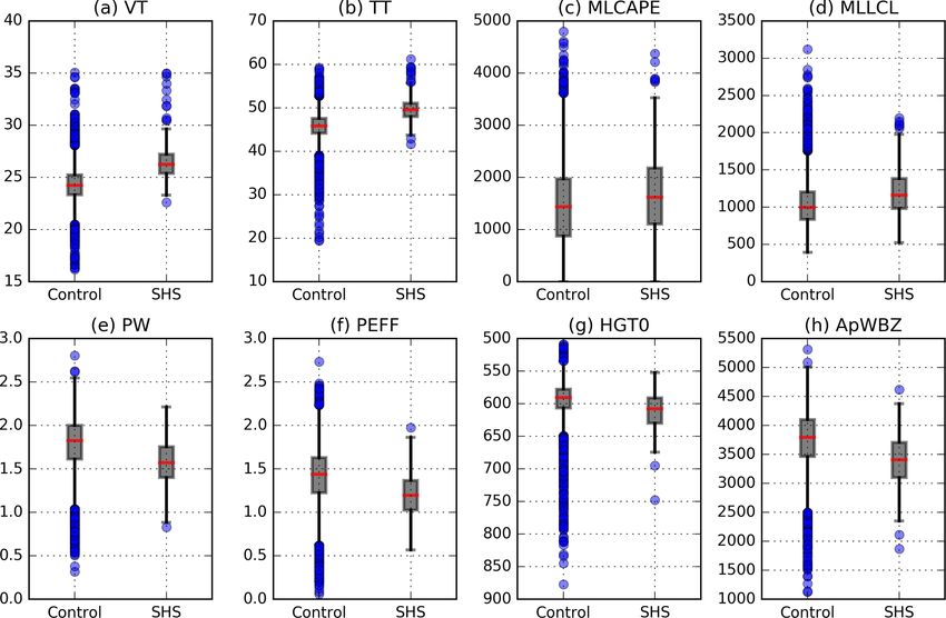
P. W. Miller and T. L. Mote: Characterizing severe weather potential                                                                    1265

                                                                       Table 3. RAP error statistics for surface-based CAPE (SBCAPE)
                                                                       and several of the variables listed in Table 2. The statistics are pre-
                                                                       sented similarly to Thompson et al. (2003) by providing the mean
                                                                       RAP-derived value, the mean arithmetic error (bias), and the mean
                                                                       absolute error (MAE).

                                                                                Parameter         Mean        Bias    MAE        R2
                                                                                SBCAPE           1354.3     141.3     530.4     0.59
                                                                                MLCAPE            943.4     112.6     338.0     0.64
                                                                                MLLCL            1077.4     −32.9     151.8     0.82
                                                                                Total totals       44.8      0.51      1.54     0.74
                                                                                TEI                21.1     −2.30      3.80     0.69
                                                                                0–3 km shear       6.33     −0.48      1.38     0.82
                                                                                0–6 km shear       8.39     −0.28      1.40     0.88

                                                                       2, the transmission of these errors onto the derived convec-
                                                                       tive parameters can be large. Table 3 expresses error mea-
                                                                       sures for surface-based (SBCAPE) and mean-layer CAPE
                                                                       (MLCAPE), 0–3 km and 0–6 km wind shear, TTs, and TEI.
                                                                       Because the focus of this study is surface-based convec-
                                                                       tion, only days when the observed surface-based CAPE was
                                                                       greater than zero were used to calculate the derived quan-
                                                                       tity error metrics. Similar to previous work (e.g., Lee, 2002),
                                                                       parameters calculated via the vertical integration of a parcel
                                                                       trajectory, such as CAPE, are sensitive to errors in low-level
                                                                       temperature and moisture. The RAP’s low-level temperature
                                                                       and moisture biases influence the lifted condensation level
                                                                       (LCL) calculation (negative MLLCL bias; Table 3) yielding
                                                                       a premature transition to the pseudo-adiabatic lapse rate and
Figure 2. Vertical profiles of RAP output errors measured by co-
located radiosonde observations (a). Errors were calculated at 1000,
                                                                       an overestimate of parcel instability (positive SBCAPE and
925, 850, 700, 500, 300, and 200 hPa. The 95 % confidence interval     MLCAPE biases; Table 3)1 . Thompson et al. (2003) iden-
for the mean error (solid lines) is shaded. Box plots of the result-   tified smaller CAPE errors generated by the RUC-2; how-
ing error for six derived quantities is shown in panels (b–d). The     ever, the nature of the thermodynamic environments being
interquartile range (IQR), representing the middle 50 % of values,     examined is significantly different in this study. Similar to
is depicted by the gray box. Values lying more than 1.5 × IQR from     the RUC-2, the RAP is more adept at representing MLCAPE
the median (red line) are marked with dots.                            than SBCAPE with Fig. 2b and, consequently, the mean-
                                                                       layer parcel trajectory will be used for all parcel-related cal-
                                                                       culations.
ing ratio confidence interval captures zero at all altitudes ex-           In some cases, RAP proxy soundings may have been con-
cept 500 hPa, where the RAP predicted drier-than-observed              taminated by premature convective overturning within the
values by 0.08 g kg−1 . Temperatures are warmer than ob-               model. However, because the RAP assimilates radar reflec-
served throughout most of the troposphere with a maximum               tivity from the US (Benjamin et al., 2016), the 0 h RAP
bias of 0.26 ◦ C at 850 hPa. In contrast, the RAP underes-             analysis fields should generally mirror the radar-observed ar-
timated wind speeds on average throughout the depth of                 eas of convection. Additionally, any such instances will be
the troposphere. The largest bias, 0.46 m s−1 , was found at           dampened by the methodological design decision to aggre-
925 hPa with similar errors above 500 hPa. The 95 % con-               gate all proxy soundings on a daily level, as will be described
fidence interval for wind speed error is largest near the              in Sect. 2.3. The accuracy of the proxy soundings could
tropopause and demonstrates larger uncertainty than for tem-           be improved by employing a convection-permitting numer-
perature and mixing ratio. These results generally agree with
the error statistics provided by Benjamin et al. (2016), and              1 The near-surface temperature and moisture errors in Fig. 2a
the reader should reference that paper for additional infor-           are more pronounced following the upgrade to RAPv2 in Febru-
mation, including validation statistics, about the RAP.                ary 2014. However, because the RAP is an operational tool and this
   Although the RAP appears to resolve temperature, mix-               work has operational relevance, no attempt was made to correct for
ing ratios, and wind speeds more accurately than the RUC-              this change.

www.nat-hazards-earth-syst-sci.net/18/1261/2018/                              Nat. Hazards Earth Syst. Sci., 18, 1261–1277, 2018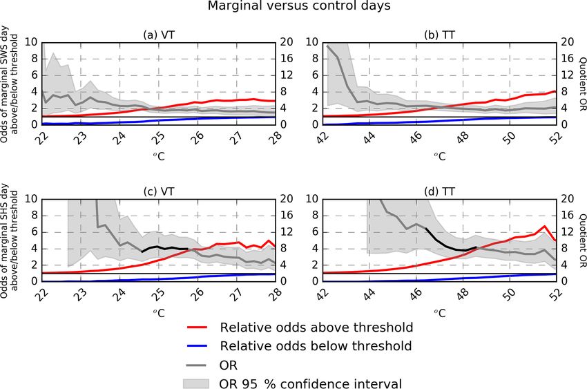
1266 P. W. Miller and T. L. Mote: Characterizing severe weather potential
Figure 3. Comparison of observed (a) vs. RAP-derived (b) soundings for a case when the MLCAPE discrepancy exceeded 1000 J kg−1
(observed: 1028 J kg−1 ; RAP: 2051 J kg−1 ). Minor mischaracterizations of low-level moisture contributed to a large response in MLCAPE
during the vertical integration of the parcel trajectory.
ical model, such as the 3 km High-Resolution Rapid Refresh the proxy soundings are subdivided by nearest radar site
(HRRR). By explicitly modeling deep convection, the HRRR (Fig. 1) and aggregated daily (12:00–12:00 UTC) by com-
would limit convective contamination by more closely repre- puting the mean parameter value associated with all WFTs
senting areas of thunderstorm activity. At the time of publi- forming within each polygon on a given day. Days containing
cation, the absence of a publicly accessible HRRR archive at least one severe weather report are considered supportive
prevented its application in this research. of severe weather, whereas days with no severe weather re-
Figure 2b–d demonstrate that although large outliers cer- ports will serve as the control. This approach is similar to the
tainly occur, the majority of RAP-derived thermodynamic methods the Hurlbut and Cohen (2013) study of severe thun-
and kinematic parameters are concentrated within a narrower derstorm environments in the Northeastern US. Severe-wind-
range of error. Figure 3 provides an example skewT-logP di- supporting (SWS) days and severe-hail-supporting (SHS)
agram for a large MLCAPE error shown in Fig. 2d. Though days are treated separately because their thermodynamic en-
the difference in this case exceeded 1000 J kg−1 , the discrep- vironments have been shown to contain unique elements
ancy can largely be attributed to the RAP’s minor mischarac- related to downdraft and hailstone production (Johns and
terization of low-level moisture. Otherwise, the depiction of Doswell, 1992). Table 4 provides the specific subdivision de-
the vertical profile is reasonably accurate. The advantage of tails of the frequency of WFT days, SWS days, SHS days,
the RAP to represent the near-storm environment is under- and their respective control days. Figure 4 shows the annual
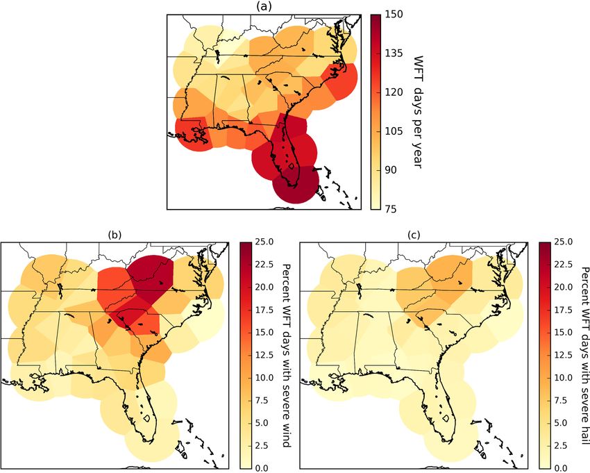
scored when compared to results from coarser-scale models. average of WFT days for each radar site within the study
For instance, the coefficients of determination (R 2 ) for RAP- area during the 2012–2015 warm seasons. As expected, WFT
derived SBCAPE and MLCAPE are appreciably larger than days are most frequent along coastlines and the Appalachian
those calculated from the 32 km horizontal and 3 h tempo- Mountains (Miller and Mote, 2017).
ral resolution North American Regional Reanalysis (NARR; Given the low SNR in WFT environments, t tests are de-
Mesinger et al., 2006) in Gensini et al. (2014). ceiving. Statistically significant differences in the mean val-
ues of parameters on severe vs. non-severe days are routinely
2.3 Assessing convective parameter skill reported, but the considerable overlap between the distribu-
tions (e.g., Craven and Brooks, 2004; Taszarek et al., 2017)
The quality of severe weather reports is a significant im- can remove much practical value. This study explores the
pediment to severe storm research (e.g., Miller et al., 2016; relationship between convective parameters and pulse thun-
Weiss et al., 2002), particularly regarding the certainty with derstorm environments by means of an odds ratio (OR; e.g.,
which non-severe storms can be declared non-severe. These Fleiss et al., 2003). The OR is a common measure of con-
storms may only appear benign because their associated se- ditional likelihood in human health and risk literature (e.g.,
vere weather was not reported. Consequently, the results of
Nat. Hazards Earth Syst. Sci., 18, 1261–1277, 2018 www.nat-hazards-earth-syst-sci.net/18/1261/2018/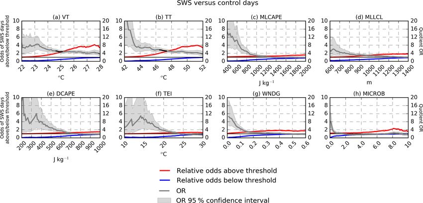
P. W. Miller and T. L. Mote: Characterizing severe weather potential                                                            1267

Figure 4. Average number of WFT days during the 4-year study period (a) compared to the proportion of WFT days affiliated with severe-
wind (b) and severe-hail (c) events.

Bland and Altman, 2000) with precedence in the atmospheric           then the odds of an SWS day are 4× greater when ML-
sciences (e.g., Black and Mote, 2015; Black et al., 2017). The       CAPE is greater than 1000 J kg−1 than when it is less than
OR looks past the descriptive statistics of the severe vs. non-      1000 J kg−1 .
severe distributions and more directly compares differences             We employ a modified form of the OR in which both the
in where the data are concentrated within the distributions.         numerator and denominator are standardized by the clima-
   Equation (1) shows the standard definition of the OR, es-         tological ratio of events to non-events (Eq. 2), allowing the
sentially the ratio of two ratios:                                   components of the OR to be separated and interpreted inde-
                                                                     pendently by comparison to climatology.
       A/C
OR =       ,                                                 (1)
       B/D                                                                       A/C
                                                                             (A+B)/(C+D)
where the numerator represents the ratio of events (A) to non-       OR =        B/D
                                                                                                                                  (2)
                                                                             (A+B)/(C+D)
events (C) when a condition is met, whereas the denominator
is the ratio of events (B) to non-events (D) when the same
condition is not satisfied. In this context, “events” are SWS           The modification does not change the value of the quotient
or SHS days whereas “non-events” would be the respective             OR, but it does improve the interpretability of the numer-
control days. Higher ORs indicate that events are more fre-          ator and denominator. When the numerator or denominator
quent (relative to non-events) when the condition is met, or         is near 0 (1), then the odds of SWS or SHS days are much
conversely, that events are less frequent when the condition is      lower than (nearly equal to) climatology. The climatological
not met. For this study, a condition might be a convective pa-       odds ratio was 0.069 for SWS days and 0.025 for SHS days.
rameter exceeding a specified threshold. For instance, if the        A 95 % confidence interval for the OR was calculated using
SWS OR equals 4 for the condition MLCAPE > 1000 J kg−1 ,             the four-step method presented in Black et al. (2017).

www.nat-hazards-earth-syst-sci.net/18/1261/2018/                            Nat. Hazards Earth Syst. Sci., 18, 1261–1277, 2018
1268                                                    P. W. Miller and T. L. Mote: Characterizing severe weather potential

Table 4. WFT, SWS, and SHS day frequency by radar site.

                  Site      WFT days     Wind control     SWS days       % SWS     Hail control   SHS days     % SHS
                  KAKQ             376            351              25        6.6           363           13       3.5
                  KAMX             581            569              12        2.1           575            6       1.0
                  KBMX             376            364              12        3.2           372            4       1.1
                  KCAE             401            339              62       15.5           377           24       6.0
                  KCLX             450            407              43        9.6           440           10       2.2
                  KDGX             426            403              23        5.4           416           10       2.3
                  KEOX             384            366              18        4.7           382            2       0.5
                  KEVX             467            449              18        3.9           463            4       0.9
                  KFCX             408            318              90       22.1           370           38       9.3
                  KFFC             400            358              42       10.5           387           13       3.3
                  KGSP             417            334              83       19.9           383           34       8.2
                  KGWX             362            349              13        3.6           354            8       2.2
                  KHPX             299            282              17        5.7           294            5       1.7
                  KHTX             373            343              30        8.0           369            4       1.1
                  KJAX             555            520              35        6.3           546            9       1.6
                  KJGX             384            356              28        7.3           377            7       1.8
                  KLIX             504            492              12        2.4           501            3       0.6
                  KLTX             452            439              13        2.9           444            8       1.8
                  KMHX             497            496               1        0.2           495            2       0.4
                  KMLB             540            532               8        1.5           532            8       1.5
                  KMOB             451            444               7        1.6           446            5       1.1
                  KMRX             415            349              66       15.9           384           31       7.5
                  KMXX             357            346               8        2.2           350            4       1.1
                  KNQA             356            336              20        5.6           345           11       3.1
                  KOHX             349            336              13        3.7           345            4       1.1
                  KPAH             330            305              25        7.6           318           12       3.6
                  KRAX             367            337              30        8.2           355           12       3.3
                  KTBW             546            525              21        3.8           535           11       2.0
                  KTLH             482            461              21        4.4           479            3       0.6
                  KVAX             457            430              27        5.9           452            5       1.1
                  Mean             425            398              27        6.7           415           10       2.5

3     Results                                                           ters are significant across much of the domain (VT and TT),
                                                                        demonstrate larger relative changes on SWS days (MLCAPE
3.1    Convective environments of pulse thunderstorm                    and MLLCL), and/or are traditional operational severe-wind
       wind events                                                      forecasting tools (DCAPE, TEI, WNDG, MICROB). How-
                                                                        ever, as the distributions clearly illustrate, any difference in
During the 4-year study period, pulse thunderstorm wind                 the mean values between the control days and SWS days is
events were documented somewhere in the study area on                   small compared to the spread about their means. This results
49 % of WFT days, although the average frequency within                 in the characteristically low SNR described in the Sect. 1.
any single subdivision was 6.7 % (Table 4). Table 5 shows the           Any attempt to establish a forecasting value indicative of
31 convective parameters analyzed from the proxy soundings              pulse-wind potential will yield many missed events occur-
as well as the number of subdivisions for which each param-             ring beneath the threshold and/or false alarms associated with
eter is a statistically significant differentiator of SWS days.         control days above it.
A significance threshold of p < 0.10 guided the selection of               Thus, Fig. 6 employs the OR to characterize the relative
potentially useful parameters which would be examined in                skill that some knowledge of the convective environment can
more detail. Nine of the 31 variables are statistically signifi-        contribute to a severe vs. non-severe designation. For each
cant across at least two-thirds of the study area: VT, TT, ML-          variable in Fig. 5, a progressively larger value is selected,
CAPE, MLLCL, MICROB, DCAPE, TEI, RH_LOW, and                            and the OR is calculated at each step. Figure 6 displays the
ThE_LOW.                                                                OR as well as both the numerator and denominator terms for
   Figure 5a–h depict the distributions for several parameters          each iteration. High ORs can often result when a near-zero
from Table 5 for control vs. SWS days. These eight parame-              number of severe events exist below the threshold inflating

Nat. Hazards Earth Syst. Sci., 18, 1261–1277, 2018                              www.nat-hazards-earth-syst-sci.net/18/1261/2018/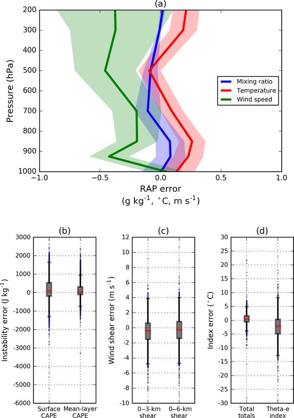
P. W. Miller and T. L. Mote: Characterizing severe weather potential                                                                 1269

Figure 5. Box plots of selected convective parameters that demonstrated skill in differentiating between the control days and SWS days.

Figure 6. ORs for the same eight convective parameters shown in Fig. 5. Whenever the OR, defined by Eq. (2), results from a numerator (red)
≥ 2 and a denominator (blue) ≤ 0.5, then the OR is drawn in black. The left y axis expresses values corresponding to the OR’s numerator and
denominator (red and blue lines), and the right y axis corresponds to the OR value (gray line). At very low and very high threshold values,
the variance of the OR may be undefined, and the 95 % OR confidence interval cannot be computed.

the OR calculation. In these situations, the OR is indicating           large ORs will result when the numerator indicates an ap-
that severe weather is very unlikely rather than that the severe        preciable increase against the climatology while the denom-
weather risk is enhanced. These results are not particularly            inator simultaneously indicates an appreciable decrease be-
useful because forecasters would not have needed a decision-            low climatology. Further, these ORs would ideally occur in
support tool in these environments in the first place. Ideally,         a range where the severe weather risk may be uncertain. In

www.nat-hazards-earth-syst-sci.net/18/1261/2018/                               Nat. Hazards Earth Syst. Sci., 18, 1261–1277, 2018
1270                                                     P. W. Miller and T. L. Mote: Characterizing severe weather potential

Table 5. Summary of convective parameters on SWS days. The           additional dew point term included. Meanwhile, MLCAPE
“sites” column indicates the number of spatial subdivisions within   and MLLCL demonstrate consistently lower ORs between 2
which the difference between the SWS mean and the control mean       and 4. The four wind-specific variables in Fig. 6e–h are rela-
was accompanied by p < 0.10; the “percent change” column shows       tively poor differentiators of SWS days in the WFT regime.
the relative increase or decrease of the mean on SWS days.           The maximum OR achieved by any of these parameters is
                                                                     approximately 10 driven by very low values of DCAPE with
             Parameter       Sites   Percent change                  corresponding wide confidence intervals.
             VT                 28              5.1                     Though ORs are greater at lower VT and TT thresholds,
             TT                 27              4.2                  these values are also somewhat common. Placing the afore-
             MLCAPE             25             31.2                  mentioned values (24.6 and 46.5 ◦ C, respectively) in the con-
             MICROB             23             44.0                  text of the 12 759 WFT environments included in this study,
             DCAPE              22             17.3                  they represent the 58.8th and 58.9th percentiles of their dis-
             TEI                22             13.1                  tributions. Alternatively, the maximum VT threshold that
             MLLCL              21             12.9
                                                                     yields a 2-fold OR is 25.1 ◦ C, which corresponds to the
             ThE_LOW            21              0.9
             RH_LOW             20             −5.5
                                                                     70.9th percentile of all VTs in the dataset; however, the OR
             WNDG               19             41.2                  for this value is smaller, 4.77. This result illustrates the trade-
             CT                 19              3.2                  off involved by seeking climatologically exceptional values
             Tc                 19              5.8                  to serve as guidance. As greater values are selected as the
             MLEL               18              8.0                  threshold, meteorologists can focus on a fewer number of
             SWEAT              14              7.8                  days. However, the OR decreases as more severe weather
             W_LOW              10              3.0                  events occur in environments not satisfying the threshold.
             K_IND               8              3.8                  As for TT, the maximum 2-fold OR value is 47.3 ◦ C, corre-
             RH_MID              7             −3.2                  sponding to the 70.6th percentile, but demonstrates an OR of
             ThE_MID             6              0.1                  5.16. This means that when TT meets or exceeds 47.3 ◦ C, the
             PEFF                6             −3.8
                                                                     odds of a pulse thunderstorm severe-wind event are 5.16×
             0–6 km_SHR          6             −4.5
             0–8 km_SHR          6             −6.5
                                                                     greater than when it does not.
             ApWBZ               5             −0.5
             HGT0                4              0.1                  3.2   Convective environments of pulse thunderstorm
             W_MID               3              0.0                        hail events
             MLBRN               3             −0.7
             NCAPE               2             23.9                  Table 6 replicates Table 5 except for SHS days. Many of
             PW                  2              0.9                  the same parameters that are statistically significant differ-
             0–3 km_SHR          2             −1.2                  entiators of SWS days also rank high for SHS days. How-
             MLCIN               0              6.6                  ever, fewer parameters in Table 6 are statistically significant
             MLLFC               0              0.9                  over two-thirds of the domain. Whereas 10 parameters in
             EBWD                0             −1.9
                                                                     Table 5 showed spatially expansive statistical skill on SWS
                                                                     days, only three quantities do so on SHS days. We attribute
                                                                     this result to the pattern in Table 4 and Fig. 4b and c whereby
Fig. 6, the OR is shown in a gray line, but the line is drawn        there are fewer SHS days than SWS days, which increases
in black whenever the OR results from a numerator ≥ 2 and            uncertainty related to the statistical tests and makes it harder
a denominator ≤ 0.5. ORs resulting from this combination             to confidently detect differences.
indicate that the threshold yields a simultaneous 2-fold in-            Nonetheless, VT and TT are once again skillful differen-
crease (decrease) in the odds of SWS days above (below) the          tiators and are now joined by their related parameter CT.
specified value. These ORs will be hereon referenced as “2-          Additionally, several new convective variables demonstrate
fold” ORs and represent a goal scenario.                             statistical significance across roughly half of the domain on
   Figures 6a–h show ORs for the same eight parameters in            SHS days that demonstrated little skill on SWS days: PW,
Fig. 5. Of all eight parameters, only VT and TT achieve 2-           PEFF, HGT0, and ApWBZ. For comparison, Fig. 7a–d du-
fold ORs for any range of thresholds, as indicated by the            plicate Fig. 5a–d, now comparing distributions between the
black segments in Fig. 6a and b. The maximum 2-fold OR               control and SHS days, while Fig. 7e–h display box plots
for VT is 5.16 at 24.6 ◦ C, meaning that the odds of an SWS          for the SHS-specific convective parameters listed above. The
day are 5.16× greater when this threshold is met. TT offers          distributions for MLCAPE and MLLCL are similar; how-
slightly more skill with a maximum 2-fold OR of 5.70 at              ever, there is a larger separation between control and SHS
46.5 ◦ C. As described in Appendix A, VTs and TT s are rela-         days for VT and TT than was apparent on SWS days. This
tively primitive indices. VT is purely a temperature lapse rate      observation is corroborated by the relative changes in VT
whereas TT is predominantly a measure of lapse rate with an          and TT on SHS days that are several percentage points larger

Nat. Hazards Earth Syst. Sci., 18, 1261–1277, 2018                           www.nat-hazards-earth-syst-sci.net/18/1261/2018/
P. W. Miller and T. L. Mote: Characterizing severe weather potential 1271
Figure 7. Same as Fig. 5 except for SHS days. Panels (a–d) replicate the same variables shown in Fig. 5, whereas (e–h) are replaced with
four SHS-specific parameters from Table 6.
than for SWS days (Table 6). PW, PEFF, HGT0, and ApWBZ storm days on the OR analysis is further scrutinized. For
demonstrate smaller differences. this purpose, “marginal” SWS and SHS days are defined as
Figure 8 replicates Fig. 6 except by representing SHS days those on which only one severe wind or hail report was re-
and substituting the four wind-specific parameters (DCAPE, ceived. Marginal days constitute 48.7 % of the SWS days and
TEI, WNDG, MICROB) with the four hail parameters listed 57.7 % of the SHS days in Table 4. Figure 9 replicates the
above (PW, PEFF, HGT0, ApWBZ). The ORs for VT and OR analysis for VT and TT, the two most promising envi-
TT are large, greater than 10, throughout the entire range ronmental parameters from Sects. 3.1 and 3.2, but with only
of thresholds tested, and contain larger swathes of 2-fold marginal SWS and SHS days being considered. Comparing
ORs. The maximum 2-fold OR for VT is 13.1 at 24.4 ◦ C, Figs. 6a and b and 8a and b to Fig. 9, marginal SWS and SHS
and the maximum VT threshold that achieves a 2-fold OR days resemble the OR patterns of the broader set of SWS
is 26.0 ◦ C with an OR of 9.61. These values relate to (Fig. 6a and b) and SHS (Fig. 8a and b) days. Though the
the 53.4th and 86.0th percentiles of the VT distribution. ORs for the marginal subset are slightly smaller than for the
As for TT, the maximum 2-fold OR is 14.98 at 46.3 ◦ C, broader group, they bear similar OR patterns as the thresh-
and the maximum 2-fold-OR threshold is 49.2 ◦ C with an olds are increased. Overall, marginal SWS and SHS days are
OR of 11.79. These two TT cutoffs translate to the 55.7th generally characterized by similar VT and TT values as when
and 88.4th percentiles. Similar to SWS days, MLCAPE all SWS and SHS days were aggregated. Corroborating this
and MLLCL show little skill with ORs generally between finding, an OR analysis comparing marginal SWS and SHS
1 and 2. PW, PEFF, HGT0, and ApWBZ perform more ca- days to those with > 1 severe event (not shown) revealed that
pably than MLCAPE and MLLCL; however, they do not ORs generally remained near 1 regardless of the VT or TT
produce any 2-fold ORs. Values for these metrics are gen- threshold selected. Thus, although marginal pulse thunder-
erally around 4 with several instances of higher ORs driven storm days are by no means easily distinguishable from non-
by a small denominator with wide 95 % confidence intervals. severe WFT days, they do not appear to be particularly more
challenging to differentiate than active pulse thunderstorm
3.3 Separating marginal pulse thunderstorm days days.
Because the severe weather generated by pulse thunder-
storms is often near the lower limit used to define severe 4 Discussion
weather in the United States, some pulse thunderstorm en-
vironments may closely resemble non-severe regimes. Con- The relative changes in the convective variables in Table 5 on
sequently, the influence of these “marginal” pulse thunder- SWS days vs. control days correspond well to previous mi-
www.nat-hazards-earth-syst-sci.net/18/1261/2018/ Nat. Hazards Earth Syst. Sci., 18, 1261–1277, 20181272 P. W. Miller and T. L. Mote: Characterizing severe weather potential Figure 8. Same as Fig. 6 except for SHS days. Panels (a–d) replicate the same variables shown in Fig. 6, whereas (e–h) are replaced with four SHS-specific parameters from Table 6. At very low and very high threshold values, the variance of the OR may be undefined, and the 95 % OR confidence interval cannot be computed. Figure 9. Same as Fig. 6a and b (a, b) and Fig. 8a and b (c, d) except that only marginal SWS and SHS days are used to calculate the OR. At very low and very high threshold values, the variance of the OR may be undefined, and the 95 % OR confidence interval cannot be computed. croburst research. Compared to the non-severe control days, face layer supports evaporative cooling, downdraft accelera- SWS days are characterized by a drier near-surface layer tion, and severe outflow winds. This same conceptual model (i.e., lower RH, higher LCLs). Simultaneously, steep mid- has been promoted by previous severe convective wind re- level lapse rates (i.e., larger VT and TT) aid an increase in search (e.g., Atkins and Wakimoto, 1991; Kingsmill and CAPE which supports stronger updrafts. As the strong up- Wakimoto, 1991; Wolfson, 1988). draft transitions to a downdraft-dominant storm, the drier sur- Nat. Hazards Earth Syst. Sci., 18, 1261–1277, 2018 www.nat-hazards-earth-syst-sci.net/18/1261/2018/
P. W. Miller and T. L. Mote: Characterizing severe weather potential                                                       1273

Table 6. Same as Table 5, except for SHS days.                     prising given their prominence in severe storm forecasting.
                                                                   One possibility is that the daily aggregation of MLCAPEs
             Parameter       Sites   Percent change                may have smoothed out locally higher values near the WFTs
             VT                27              8.0
                                                                   that were responsible for severe weather production. Alter-
             TT                27              7.5                 natively, VT and TT were among the strongest indicators
             CT                21              7.1                 of both SWS and SHS days. Recalling from Sect. 2.2, VT
             PEFF              16            −11.0                 and TT are also very well represented by the RAP. TTs were
             MLLCL             15             13.2                 replicated by the model with a < 1 ◦ C bias and a MAE repre-
             HGT0              14              2.4                 senting only 3 % of the average value (Table 3). Additionally,
             ApWBZ             14             −6.0                 mid-level temperatures, from which VT is computed, also
             RH_LOW            14             −5.3                 compared very well to the observed soundings (Fig. 2a). The
             DCAPE             13             23.3                 strong performance of VT and TT compared to other more
             MLCAPE            12             28.8                 heavily moisture-weighted metrics may be due to their more
             PW                12             −6.7
                                                                   accurate representation in the proxy soundings.
             W_MID             11             −9.2
             ThE_MID           10             −0.7
                                                                      Regardless, because the severe weather SNR is already
             WNDG              10             27.4                 low in WFT environments, any systematic error introduced
             RH_MID             9             −7.8                 by the data source (in this case the RAP) may significantly
             TEI                7             10.4                 dampen, or even remove, whatever environmental differ-
             MICROB             7             21.6                 ences exist. As Sect. 2.2 indicated and previous work has
             SWEAT              7             10.1                 also concluded, low-level moisture biases can impede the ac-
             W_LOW              6             −2.1                 curate calculation of convective parameters relying on those
             Tc                 6              3.2                 terms (e.g., Gensini et al., 2014; Thompson et al., 2003). In
             0–6 km_SHR         6              9.7                 this study, MLCAPE, MLLCL, PW, PEFF, and others were
             0–8 km_SHR         5              6.9                 vulnerable to such errors. The poorer performance of these
             MLEL               4              3.8
                                                                   variables’ ORs (relative to the lapse-rate-based parameters)
             K_IND              3              2.7
             ThE_LOW            3             −0.1
                                                                   and the sensitivity of PW, PEFF, and ApWBZ to simulated
             0–3 km_SHR         3              5.3                 RAP errors suggests that model inaccuracies may be ob-
             NCAPE              1             27.0                 scuring their potential skill to detect weakly forced severe
             MLCIN              1             17.7                 weather environments. The perception of the WFT environ-
             MLLFC              1              4.1                 ment as a difficult-to-forecast regime may partly be driven by
             MLBRN              1            −15.8                 model inconsistency exacerbating an already small SNR.
             EBWD               1              9.5                    Another confounding factor is the quality of the Storm
                                                                   Data severe weather reports. Section 3.3 discussed that
                                                                   marginal SWS and SHS days are more similar to days
                                                                   with > 1 report than days with no reports. Thus, the basis for
   The results of SHS days also support previous findings          the similarity may be that severe weather was simply under-
(Johns and Doswell, 1992; Moore and Pino, 1990; Púčik             reported on “marginal” days. Extending this logic, the pulse
et al., 2015). The distributions in Fig. 7 (and relative changes   regime’s low SNR may also be partially attributed to under-
in Table 6) indicate that SHS days are characterized by rel-       reporting of severe weather on “non-severe” days. Given
ative decreases in PW, a lower freezing level, a lower wet-        that the severe weather generated by pulse convection is of-
bulb freezing level, and dry near-surface air. Smaller PWs re-     ten short-lived, isolated, and narrowly exceeds severe crite-
sult in less waterloading and greater parcel buoyancy (larger      ria, the notion that some pulse-related severe weather events
VT, TT, and MLCAPE), which maximizes updraft strength.             go undetected is likely. If some “non-severe” days existing
Meanwhile, lower freezing levels and a dry layer between           above the tested parameter thresholds in Figs. 6 and 8 did
1000 and 850 hPa support evaporative cooling which can to-         in fact host severe weather, then the ORs would have been
gether yield a lower wet-bulb zero height and limit hail stone     larger than those found in Sects. 3.1 and 3.2.
melting during its descent to the surface. Interestingly, these
two concepts are both represented in the PEFF calculation
(Appendix A), which was not developed as a hail indicator.         5   Conclusions
PEFF as defined by Noel and Dobur (2002) equals the prod-
uct of PW and the mean 1000–700 hPa RH. As both values             Hazardous weather within WFT environments is character-
decrease, PEFF becomes smaller and hail is more likely for         ized by a lower SNR than other severe thunderstorm regimes.
the reasons stated above.                                          Though past research has developed promising tools for
   The poor performance of MLLCLs and MLCAPEs in dif-              forecasting pulse thunderstorm environments, their relatively
ferentiating SWS and SHS days from their controls is sur-          small samples sizes may have understated the SNR and, by

www.nat-hazards-earth-syst-sci.net/18/1261/2018/                         Nat. Hazards Earth Syst. Sci., 18, 1261–1277, 2018
1274 P. W. Miller and T. L. Mote: Characterizing severe weather potential
corollary, overstated the reliability of their tools. With re- The noteworthy performance of VT and TT, two quanti-
cent research suggesting that the performance of new severe ties calculated from the more reliable RAP output fields, is
weather forecasting tools is closely tied to the proportion of unlikely a coincidence. Our findings suggest that the already
non-severe thunderstorms in the sample (Murphy, 2017), this weak severe weather SNR in WFT environments is exac-
study sought to test the relative skill of 31 convective fore- erbated by model limitations in the low-level moisture and
casting parameters using realistic proportions of severe and temperature fields. Meteorologists may perhaps alleviate the
non-severe WFT environments (severe: 7.9 %; non-severe: challenges of the WFT environment by examining convective
92.1 %). Future research may consider broadening the meth- parameters that are well-represented by models, such as VT,
ods of Murphy (2017) to standardize the skill values across TT, and other measures of lapse rate. Future research might
previous studies of severe convective environments. seek to track the transmission of the model errors through
Only 13 (5) of the 31 convective parameters tested were calculation of forecast skill statistics and more concretely as-
statistically significant (p < 0.10) differentiators of SWS certain the contribution of model error to the SNR.
(SHS) days across at least half of the domain. Though the
distinctive variables for SWS and SHS days were consistent
with previous theories of severe microburst and hail forma- Data availability. The radar archive used to identify thunderstorm
tion, considerable overlap between the distribution of values activity over the Southeastern US is maintained by the United
on severe and non-severe days is problematic. Similarities States National Centers for Environmental Information (NCEI), and
between the SWS, SHS, and their corresponding control dis- can be accessed via the following publicly available URL: https:
//www.ncdc.noaa.gov/nexradinv/ (NCEI, 2018). The NCEI also
tributions inhibit consistent identification of pulse thunder-
hosts a publicly accessible database of Rapid Refresh analyses (ftp:
storm potential based on the value of any individual param-
//nomads.ncdc.noaa.gov/RUC/analysis_only/, NCEP, 2018), which
eter. Nonetheless, VT and TT did perform more skillfully were used to construct the proxy soundings.
than the others. When VTs exceed values between 24.6 and
25.1 ◦ C or TTs between 46.5 and 47.3 ◦ C, the relative odds
of a wind event increases roughly 5×. Meanwhile, the odds
of a hail event become roughly 10× greater when VTs ex-
ceed values between 24.4 and 26.0 ◦ C or TTs between 46.3
and 49.2 ◦ C.
Nat. Hazards Earth Syst. Sci., 18, 1261–1277, 2018 www.nat-hazards-earth-syst-sci.net/18/1261/2018/P. W. Miller and T. L. Mote: Characterizing severe weather potential 1275
Appendix A:
Table A1. Additional detail describing the convective parameters in
Table 2.
Parameter Comments
MLCAPE
MLCIN
MLLCL Mean-layer parcel mixed over the lowest 100 hPa
MLLFC
MLEL
NCAPE MLCAPE/MLEL
K_IND T850 − T500 + Td850 − (T700 − Td700 )
TT CT + VT
CT Td850 − T500
VT T850 − T500
PW Depth of liquid water if all water vapor were condensed from the sounding
HGT0 Pressure level of the 0 ◦ C isotherm
ApWBZ Height above ground level of the RAP pressure level with the wet bulb temperature nearest to 0 ◦ C
W_LOW Mean mixing ratio between 1000 and 850 hPa
W_MID Mean mixing ratio between 850 and 500 hPa
RH_LOW Mean RH between 1000 and 850 hPa
RH_MID Mean RH between 850 and 500 hPa
ThE_LOW Mean θe from 1000 to 850 hPa
ThE_MID Mean θe from 850 to 500 hPa
ML_BRN Bulk Richard number of the mean-layer parcel
Tc Temperature of parcel lowered dry adiabatically from the convective condensation level
PEFF As defined by Noel and Dobur (2002). PEFF equals the product of PW and the mean 1000–700 hPa RH.
DCAPE Downdraft CAPE with respect to parcel with the minimum 100 hPa layer-averaged θe found in the lowest
400 hPa of the sounding.
WNDG (MLCAPE)/2000·(0–3 km lapse rate)/9·(1–3.5 km mean wind)/15·[(MLCIN +50)/40]. Values larger than 1
indicate an increased risk for strong outflow gusts.
TEI Difference between the surface θe and the minimum θe value in the lowest 400 hPa a.g.l.
MICROB Weighted sum of the following individual parameters: surface θe , SBCAPE, surface-based lifted index, 0–3 km
lapse rate, VT, DCAPE, TEI, and PW. Values exceeding 9 indicate that microbursts are likely.
SWEAT 12(Td850 ) + 20(T T − 49) + 2(U850 ) + (U500 ) + 125[sin(Udir500 − Udir850 ) + 0.2]
0–3 km_SHR Magnitude of vector shear between surface and 3 km a.g.l.
0–6 km_SHR Magnitude of vector shear between surface and 6 km a.g.l.
0–8 km_SHR Magnitude of vector shear between surface and 8 km a.g.l.
EBWD Magnitude of vector shear between effective inflow base and one half of the MU equilibrium level height
www.nat-hazards-earth-syst-sci.net/18/1261/2018/ Nat. Hazards Earth Syst. Sci., 18, 1261–1277, 20181276 P. W. Miller and T. L. Mote: Characterizing severe weather potential
Competing interests. The authors declare that they have no conflict Guillot, E. M., Smith, T. M., Lakshmanan, V., Elmore, K. L.,
of interest. Burgess, D. W., and Stumpf, G. J.: Tornado and severe thunder-
storm warning forecast skill and its relationship to storm type, in:
24th Int. Conf. Interactive Information Processing Systems for
Acknowledgements. The authors thank Alan Black, Tomas Pucik, Meteor., Oceanogr., and Hydrol., New Orleans, LA, 4A.3, avail-
and an anonymous reviewer for providing comments on earlier able at: http://ams.confex.com/ams/pdfpapers/132244.pdf (last
drafts of the manuscript. access: 24 April 2018), 2008.
Hamlington, B. D., Leben, R. R., Nerem, R. S., and
Edited by: Uwe Ulbrich Kim, K. Y.: The effect of signal-to-noise ratio on the
Reviewed by: Tomas Pucik and one anonymous referee study of sea level trends, J. Climate, 24, 1396–1408,
https://doi.org/10.1175/2010JCLI3531.1, 2010.
Hurlbut, M. M. and Cohen, A. E.: Environments of Northeast
U.S. severe thunderstorm events from 1999 to 2009, Weather
Forecast., 29, 3–22, https://doi.org/10.1175/WAF-D-12-00042.1,
References 2013.
James, R. P. and Markowski, P. M.: A numerical investigation of the
Atkins, N. T. and Wakimoto, R. M.: Wet microburst activity over effects of dry air aloft on deep convection, Mon. Weather Rev.,
the southeastern United States: implications for forecasting, 138, 140–161, https://doi.org/10.1175/2009MWR3018.1, 2010.
Weather Forecast., 6, 470–482, https://doi.org/10.1175/1520- Johns, R. H. and Doswell, C. A. I.: Severe local storms forecasting,
0434(1991)0062.0.CO;2, 1991. Weather Forecast., 7, 588–612, https://doi.org/10.1175/1520-
Benjamin, S. G., Dévényi, D., Weygandt, S. S., Brundage, K. J., 0434(1992)0072.0.CO;2, 1992.
Brown, J. M., Grell, G. A., Kim, D., Schwartz, B. E., Kingsmill, D. E. and Wakimoto, R. M.: Kinematic, dy-
Smirnova, T. G., Smith, T. L., and Manikin, G. S.: namic, and thermodynamic analysis of a weakly sheared
An hourly assimilation–forecast cycle: the RUC, Mon. severe thunderstorm over northern Alabama, Mon.
Weather Rev., 132, 495–518, https://doi.org/10.1175/1520- Weather Rev., 119, 262–297, https://doi.org/10.1175/1520-
0493(2004)1322.0.CO;2, 2004. 0493(1991)1192.0.CO;2, 1991.
Benjamin, S. G., Weygandt, S. S., Brown, J. M., Hu, M., Alexan- Lee, J. W.: Tornado Proximity Soundings from the NCEP/NCAR
der, C. R., Smirnova, T. G., Olson, J. B., James, E. P., Reanalysis Data, M.S., Dept. of Meteorology, University of Ok-
Dowell, D. C., Grell, G. A., Lin, H., Peckham, S. E., lahoma, Norman, OK., 61 pp., 2002.
Smith, T. L., Moninger, W. R., Kenyon, J. S., and Manikin, G. S.: McCann, D. W.: WINDEX – a new index for
A North American hourly assimilation and model forecast cy- forecasting microburst potential, Weather Fore-
cle: the Rapid Refresh, Mon. Weather Rev., 144, 1669–1694, cast., 9, 532–541, https://doi.org/10.1175/1520-
https://doi.org/10.1175/MWR-D-15-0242.1, 2016. 0434(1994)0092.0.CO;2, 1994.
Black, A. W. and Mote, T. L.: Characteristics of winter- Mesinger, F., DiMego, G., Kalnay, E., Mitchell, K., Shafran, P. C.,
precipitation-related transportation fatalities in the United States, Ebisuzaki, W., Jović, D., Woollen, J., Rogers, E., Berbery, E. H.,
Weather Clim. Soc., 7, 133–145, https://doi.org/10.1175/WCAS- Ek, M. B., Fan, Y., Grumbine, R., Higgins, W., Li, H.,
D-14-00011.1, 2015. Lin, Y., Manikin, G., Parrish, D., and Shi, W.: North Ameri-
Black, A. W., Villarini, G., and Mote, T. L.: Effects of rainfall on can regional reanalysis, B. Am. Meteorol. Soc., 87, 343–360,
vehicle crashes in six U.S. states, Weather Clim. Soc., 9, 53–70, https://doi.org/10.1175/bams-87-3-343, 2006.
https://doi.org/10.1175/WCAS-D-16-0035.1, 2017. Miller, P. and Mote, T.: A climatology of weakly forced and pulse
Bland, J. M. and Altman, D. G.: The odds ratio, BMJ, 320, 1468, thunderstorms in the Southeast United States, J. Appl. Meteo-
https://doi.org/10.1136/bmj.320.7247.1468, 2000. rol. Clim., 56, 3017–3033, https://doi.org/10.1175/JAMC-D-17-
Blumberg, W. G., Halbert, K. T., Supinie, T. A., Marsh, P. T., 0005.1, 2017.
Thompson, R. L., and Hart, J. A.: SHARPpy: an open source Miller, P. W., Black, A. W., Williams, C. A., and Knox, J. A.: Quan-
sounding analysis toolkit for the atmospheric sciences, B. Am. titative assessment of human wind speed overestimation, J. Appl.
Meteorol. Soc., 98, 1625–1636, https://doi.org/10.1175/BAMS- Meteorol. Clim., 55, 1009–1020, https://doi.org/10.1175/JAMC-
D-15-00309.1, 2017. D-15-0259.1, 2016.
Cerniglia, C. S. and Snyder, W. R.: Development of Warning Cri- Moore, J. T. and Pino, J. P.: An interactive method for es-
teria for Severe Pulse Thunderstorms in the Northeastern United timating maximum hailstone size from forecast soundings,
States Using the WSR-88 D, National Weather Service, Albany, Weather Forecast., 5, 508–525, https://doi.org/10.1175/1520-
NY, 2002. 0434(1990)0052.0.CO;2, 1990.
Craven, J. P. and Brooks, H. E.: Baseline climatology of sounding Murphy, M.: Preliminary results from the inclusion of lightning type
derived parameters associated with deep, moist convection, Natl. and polarity in the identification of severe storms, in: 8th Conf.
Wea. Dig., 28, 13–24, 2004. on the Meteor. Appl. of Lightning Data, Seattle, WA, 22–26 Jan-
Fleiss, J. L., Levin, B., and Paik, M. C.: Statistical Methods for uary 2017, 1–12, 2017.
Rates and Proportions, Wiley, Hoboken, N.J., 2003. NCEI: NEXRAD data archive, inventory and access, available
Gensini, V. A., Mote, T. L., and Brooks, H. E.: Severe- at: https://www.ncdc.noaa.gov/nexradinv/, last access: 24 April
thunderstorm reanalysis environments and collocated ra- 2018.
diosonde observations, J. Appl. Meteorol. Clim., 53, 742–751,
https://doi.org/10.1175/JAMC-D-13-0263.1, 2014.
Nat. Hazards Earth Syst. Sci., 18, 1261–1277, 2018 www.nat-hazards-earth-syst-sci.net/18/1261/2018/You can also read