WEATHER SHOCKS, FOOD PRICES AND FOOD SECURITY: EVIDENCE FROM SOUTH AFRICA - AGECON SEARCH

Weather shocks, food prices and food security: Evidence
 from South Africa

 Kubik Z¹, May J²

¹Center For Development Research (ZEF), ²DST-NRF Centre of Excellence in Food Security
Corresponding author email: zkubik@uni-bonn.de

Abstract:
In this paper, we analyze the food access dimension of food security, and we model the link between weather
shocks and food security that acts specifically through food prices. We focus on dietary diversity as a
measure of food security, and we employ an instrumental variable model where household dietary diversity
is determined by food prices instrumented with standardized precipitation evapotranspiration index (SPEI),
a measure of weather shock. Our findings suggest that food prices have a significant negative impact on
household food security, i.e. a one per cent increase in local food prices induced by a weather shock
decreases the number of food items consumed by household by around 2.5 per cent, and the number of food
groups by almost one per cent. The low-income households are particularly vulnerable to weather and
price shocks; however, their response to shocks seem to depend on the level of poverty. The moderately
poor households from the second wealth quartile show the greatest response to shocks, but the extremely
poor household from the first wealth quartile have little scope to decrease their dietary diversity which is
already very low. While own food production might alleviate food insecurity of the poorest, it does not
insulate them form the weather and food price shocks. Our findings are robust to employing self-reported
measures of food security.
 #33

Weather shocks, food prices and food security:

 Evidence from South Africa

 Abstract
In this paper, we analyze the food access dimension of food security, and we model the link between
weather shocks and food security that acts specifically through food prices. We focus on dietary diversity
as a measure of food security, and we employ an instrumental variable model where household dietary
diversity is determined by food prices instrumented with standardized precipitation evapotranspiration
index (SPEI), a measure of weather shock. Our findings suggest that food prices have a significant
negative impact on household food security, i.e. a one per cent increase in local food prices induced by a
weather shock decreases the number of food items consumed by household by around 2.5 per cent, and
the number of food groups by almost one per cent. The low-income households are particularly
vulnerable to weather and price shocks; however, their response to shocks seem to depend on the level of
poverty. The moderately poor households from the second wealth quartile show the greatest response to
shocks, but the extremely poor household from the first wealth quartile have little scope to decrease their
dietary diversity which is already very low. While own food production might alleviate food insecurity of
the poorest, it does not insulate them form the weather and food price shocks. Our findings are robust to
employing self-reported measures of food security.

 1

Introduction

Over the last year, the state of food security has deteriorated in many parts of sub-Saharan Africa

and South-Eastern and Western Asia, according to a recent FAO report. After a prolonged

decline over a decade, the global hunger is once again on the rise, and climate-related shocks are

considered to be amongst the factors that have contributed to this reversal of trends (FAO, IFAD,

UNICEF, WFP & WHO, 2017). Climate change, expected to entail greater rainfall and

temperature variability and increased incidence of extreme events (IPCC, 2007), constitutes an

important challenge to food security particularly in developing countries which are already

vulnerable to hunger and undernutrition (Wheeler and von Braun, 2013; Parry et al., 1999). Not

only will these areas face the most adverse effects of climate change in the near future (Mora et

al., 2013), but also, their exposure to weather risk is substantial as a result of dependence on rain-

fed agriculture, while, at the same time, their adaptive capacity remains low due to financial

constraints (Ringler et al., 2010).

Starting with the seminal paper by Rosenzweig and Parry (1994), the potential impact of climate

change on agricultural productivity in sub-Saharan Africa has been thoroughly analyzed. Despite

uncertainty observed in different projections and the underlying climate models, a consistent

pattern has emerged in the literature. The lowest-income tropical countries are expected to incur

the sharpest losses (Parry et al., 1999; WB, 2010; Deryng, Sacks, Barford & Ramankutty, 2011),

especially given that crops such as maize, cassava, yam, plantain sorghum, wheat and millet, the

top sources of calories on the continent, seem to be particularly sensitive to weather extremes

(Schlenker & Lobell, 2010; Lobell et al., 2008). Several meta-analyses provided a robust

evidence of the projected decreases in yields (Müller et al., 2011; Roudier et al., 2011; Knox et

 2

al., 2012); for example, yields across Africa are expected to decline by 17 per cent for wheat, 15

per cent for sorghum, 10 per cent for millet and 5 per cent for maize (Knox et al., 2012), with

important regional differences (Lobell et al., 2008). The assessment of the adverse impact of

climate change on agricultural productivity would potentially be even more distressing if

changes in livestock, fisheries, and other crops, such as vegetables or pulses, which play a minor

role globally but might be relevant at a local level, were accounted for (Wheeler & von Braun,

2013; Campbell et al., 2016).

Accordingly, even though food security is an inherently complex concept, as reflected in the

multidimensional FAO definition encompassing food availability, access, utilization and stability

(FAO, 1996), the debate on climate change and food security has focused on one aspect, that is

food supply or availability (Wheeler & von Braun, 2013; Campbell et al., 2016). However, since

the remaining components of food security are expected to be affected by climate change as well,

it is necessary to include them in the analysis by adopting the food system approach rather than

focusing on food production alone (Porter et al., 2014; Vermeulen, Campbell, & Ingram, 2012).

One of the main indirect channels through which climate-related shocks might undermine food

security is the change in levels and volatility of food prices that, in turn, is a key determinant of

food access (Porter et al., 2014). In the climate change context, the IFPRI ‘business-as-usual

projections’ anticipate a rise in prices of most cereals and meats, reversing long-established

downward trends. For example, the price of maize is projected to increase by 104 per cent

between 2005 and 2050 if no technology adoption is taken into account (Rosegrant et al., 2014).

Declines in yields and production due to climate change are expected to significantly contribute

 3

to imbalances in supply and demand, together with the population and income growth on the

demand side (Nelson et al., 2010; Godfray et al., 2010).

Weather shocks are only one of the interlinking domestic and external factors affecting food

prices (Headey & Fan, 2010). Literature on domestic food prices in developing countries has

also focused on aspects such as market integration and price transmission (see Abdulai, 2000;

Rashid, 2004; Minot, 2011; Burke & Myers, 2014). Even though the systematic analysis of the

relationship between weather shocks and domestic food prices is rather limited (Mirzabaev &

Tsegai, 2012), the available evidence clearly suggests that in the context of many local markets

in developing countries, domestic weather shocks are a major source of short-term food price

variability. As a result of a limited scope of market integration, weather shocks have been shown

exert a greater influence than external shocks (Baffes, Kshirsagar, & Mitchell, 2015; Brown &

Kshirsagar, 2015).

Since they are endogenous outcomes of underlying market forces, prices cannot be considered as

a fundamental cause of changes in food security conditions (Kalkuhl, von Braun, & Torero,

2016); nevertheless, they are likely to signal food security risks (Ringler et al., 2010). Since the

share of food in the total budget of the poor amounts to two-thirds (Cranfield, Eales, Hertel, &

Preckel, 2003), a change in food prices implies a change in real income, but whether this change

is positive or negative depends on a household’s net food position, with higher food prices

expected to harm the net buyers but benefit net sellers of food (Deaton, 1989). Taking into

account that in many low- and middle-income countries, the poor are typically net food buyers,

albeit often only marginally so (Aksoy & Isik-Dikmelik, 2008), it is generally expected that

 4

increases in real food prices entail negative consequences in terms of welfare (de Hoyos &

Medvedev, 2011; Ivanic & Martin, 2014). The long-term secondary effects on labour market

and wages introduce further complexity (Ravallion, 1989; Hertel, 2016; Headey & Martin,

2016).

In the short run, the evidence suggests that food price shocks adversely affect food security, and

particularly so in case of the poorest households (Alem & Söderbom, 2012; Akter & Basher,

2014). In response to food price shocks, households adjust their consumption patterns in a

number of ways: by decreasing caloric intake (Robles & Torero, 2010; Tiwari & Zaman, 2010;

Anríquez, Daidone, & Mane, 2013), decreasing number of meals per day (Matz, Kalkuhl, &

Abegaz, 2015), decreasing food diversity (Hertel, 2016), or substituting with less preferred foods

(Matz et al., 2015). More importantly, even temporary disruptions in food access resulting from

food inflation can entail long-term, often irreversible nutritional damage, especially amongst

infants and young children in the period critical for growth and development (Robles & Torero,

2010; de Brauw, 2011; Arndt et al., 2016).

Therefore, if weather shocks translate into food price shocks which, in turn, adversely affect food

security, then the ongoing climate change should be considered as an important risk. This

extends beyond subsistence households relying on own food production, as commonly assumed

in the literature, but also, to net food buyers. This question has been addressed mainly in the

macroeconomic setting; for example, Badolo and Kinda (2012) find evidence that rainfall

volatility is a factor of food insecurity particularly in sub-Saharan Africa, and that this adverse

effect of weather shocks is exacerbated for countries that are vulnerable to food price shocks.

 5

Ringler et al. (2010) predict that as a result of climate change and consecutive price increases,

caloric intake in Africa will decrease while the number of malnourished children will increase.

Similar results are obtained for South Asia (Bandara & Cai, 2014). Several microeconomic

studies, even though they do not address the weather shocks – prices – food security link in

detail, find evidence of a non-negligible impact of adverse weather conditions on food security

outcomes. Weather shocks have been associated with lower child growth (Hoddinott & Kinsey,

2001), malnutrition (Jensen, 2000) and nutrient deficiencies in pregnant women (Gitau et al.,

2005).

In this paper, we analyze the food access dimension of food security, and we model the link

between weather shocks and food security that acts specifically through food prices. First, we

assume that negative weather shocks affect agricultural productivity and lead to a decrease in

local food supply. This reduction in food supply is then likely to entail an increase in domestic

food prices. Second, we expect the increase in food prices to negatively affect household food

security, or, more specifically, its access dimension. This study is a departure from existing

approaches focusing only on the direct impact of weather shocks on food availability in sub-

Saharan Africa to consider the situation in which a large share of households are net food buyers.

This is so the case of South Africa and will increasingly be relevant in other middle income

countries in an urbanizing Africa (May, 2017). We focus on dietary diversity as a measure of

food security, and we employ an instrumental variable model where household dietary diversity

is determined by food prices instrumented with standardized precipitation evapotranspiration

index (SPEI), our measure of weather shock. Our findings suggest that food prices have a

significant negative impact on household food security, i.e. a one per cent increase in local food

 6

prices induced by a weather shock decreases the number of food items consumed by household

by around 2.5 per cent, and the number of food groups by almost one per cent. In line with

expectations, the low-income households are particularly vulnerable to weather and price shocks;

however, their response to shocks seem to depend on the level of poverty.

Background

For several reasons, South Africa is a distinctive case study in terms of food security analysis,

and in particular, its access dimension, in comparison to other countries in sub-Saharan Africa.

With its overall surplus agricultural production and the net food exporter status (Rakotoariosa,

Iafrate, & Paschali, 2011), South Africa is considered to be food-secure at the national level

(BFAP, 2012). Nevertheless, the country is confronted with substantial food insecurity at the

household level (StatsSA, 2012). Hendriks (2005) estimates that more than half of South African

households may experience some form of food insecurity. The 2011 General Household Survey

(GHS) indicates that 11.5 per cent of the sampled households reported experiencing hunger

(StatsSA, 2012), and even though this proportion has been falling over years, it represents close

to ten million people (Hendriks, 2013). However, the biggest challenge for South African food

security remains persistent undernutrition or “hidden hunger” resulting from diets lacking the

quality and variety of foods necessary to meet nutritional requirements (Altman, Hart, & Jacobs,

2009).

In this context, food insecurity in South Africa should be seen not as food availability failure, but

rather as a livelihood failure (Devereux & Maxwell, 2001) that substantially undermine

 7

households’ food access (Altman et al., 2009). Indeed, this dimension of food security seems to

be particularly important in case of South Africa where most households, both urban and rural,

are net food buyers (Hendriks & Maunder, 2006) and where food expenditures account for up to

80 per cent in case of the low-income households (Baiphethi & Jacobs, 2009). The role of own

food production is very limited as a result of a highly dualistic nature of the agricultural sector,

with around 35,000 large-scale farms (Aliber & Cousins, 2013) producing almost all marketed

output (Vink & van Rooyen, 2009); and around 2.5 million black households involved in small-

scale farming (Aliber & Hall, 2010), of which only around 200,000 derive any monetary income

from these activities (Aliber & Cousins, 2013). Additionally, a considerable movement in and

out of agriculture over years suggests that farming is considered as rather residual activity by

most households (Aliber & Hart, 2009). More importantly, rural households, including

subsistence farmers, are increasingly reliant on food purchases, i.e. more than 90 per cent of rural

households purchase most of the grain, meat and dairy products they consume from formal

retailers, and this number is only lower in case of vegetables (Baiphethi & Jacobs, 2009);

consequently, agricultural production does not significantly increase household food security

unless home production exceeds subsistence (Hendriks, 2003; Kirsten et al., 1998).

Therefore, household purchasing power, determined by household livelihood strategy and

income on the one hand, and market prices on the other, is the key to understand food security

(Altman et al., 2009; Webb et al., 2006). Several studies pointed to the rising food prices as a

food security risk in South Africa (Hendriks, 2005; Altman et al., 2013; Hart, 2009), with

particularly dire consequences for the poorest households who experience greater inflation rates

than richer ones (FPMC, 2004), and disproportionately so in rural areas where retail prices are

 8

typically much higher than in urban areas (Watkinson & Kakgetla, 2002, cited by Hendriks,

2005; Altman et al., 2009). Additionally, weather shocks, and droughts especially, are identified

as a compounding factor of food insecurity (Hendriks, 2013; Webb et al., 2006; Fraser, Monde,

van Averbeker, 2003; Mekuria & Moletsane, 1996). Indeed, extreme climate events such as

droughts, floods, cyclones, and veld fires are already seriously affecting the country, putting a

strain on agriculture and water resources; for example, the country has recently experienced the

worst drought disaster in more than a century (Archer et al., 2017). Over the past five decades,

mean annual temperatures have increased by 50 per cent more than the observed global average

of 0.65℃ while rainfall has become more disparate (Ziervogel et al., 2014); and this trend is

expected to continue under the climate change scenarios, i.e. a warming of over 2.5º, and in

some areas well over 3º, is projected by 2050 (Johnston et al., 2013). This will have serious

implications for agricultural yields, especially in case of staples such as maize (Lobell et al.,

2011; Schulze, Kiker, & Kunz, 1993), and water demand for irrigation (Ziervogel et al., 2014),

and might translate into local food prices (Vink & Kirsten, 2002).

Data

The analysis is based in the Income and Expenditure Survey (IES) and Living Conditions Survey

(LCS) administered by Statistics South Africa (StatsSA), South Africa’s national statistics

organization.. Both the IES and LCS use the diary method for recording food expenditures, but

additionally, they also provide a data on household characteristics. We use 2005/06 and 2010/11

waves of the IES and 2008/09 and 2014/15 waves of the LCS, each of them being nationally

representative and covering between 21,000 and 25,000 households, which produces a pooled

 9

cross-section of almost 95,000 households for which we have all the required information. Of

course, ideally, we would have a panel dataset to observe changes in consumption patterns over

years within the same households (see, for example, Matz et al., 2015); nevertheless, we believe

that the variation in weather and prices between different survey years will enable us to capture

the impact of these shocks on food security. Importantly, earlier waves of the IES has previously

been used in other studies on food security (Rose, Bourne, & Bradshaw, 2002; Rose & Charlton,

2002), producing estimates comparable with the literature (Hendriks, 2005).

We employ dietary diversity as our main measure of food security, and this choice is dictated by

several reasons. First of all, dietary diversity is a well-recognized and attractive indicator of food

access (Hoddinott & Yohannes, 2002; Swindale & Bilinsky, 2006; Kennedy, Ballard, & Dop,

2011), and precisely this dimension of food security is the focus of the present paper. Second,

since the typical South African diet is energy dense but micronutrient poor (Shisana et al., 2013,

cited by Hendriks, 2014), dietary diversity, a proxy of nutrient adequacy (Swindale & Bilinsky,

2006), is more relevant than other measures, such as caloric intake. Besides, it is well established

that dietary diversity is correlated with different indictors of food security, such as energy

availability, birth weight or child anthropometric status (Hoddinott, 1999; Hoddinott &

Yohannes, 2002; Swindale & Bilinsky, 2006), also in the case of South Africa (Charlton & Rose,

2002). Last but not least, the availability of detailed expenditure records in our faciliaties

computing dietary diversity rather than other measures. We employ two indicators of dietary

diversity, i.e. a simple count of various food items consumed by the household over a reference

 10

period1 as well as Household Dietary Diversity Score (HDDS), i.e. the number of different food

groups consumed (see Kennedy, Ballar, & Dop, 2011 for details), which is expected to better

reflect the quality of a diet (Swindale & Bilinsky, 2006). Additionally, we also conduct the

analysis of food composition, i.e. the share of different food groups in total consumption; and we

use self-reported measures of food insecurity as a robustness check. The monthly data on retail

prices were obtained from StatsSA. These series are incomplete for some years in case of maize,

which is our proxy of food prices, and the missing observations were imputed using the CPI for

cereals, also obtained from StatsSA. We compute the mean price per kilogram, and we employ

this measure at the country level, and, alternatively, at the province level. The province level data

are available only starting from 2008; similarly, the missing observations were imputed using the

province-level CPI for cereals. Additionally, we also check the results for commodity price, i.e.

SAFEX white maize spot price obtained from Johannesburg Stock Exchange (JSE).

Our principal measure of weather shock is the Standardized Precipitation Evapotranspiration

Index (SPEI)2 obtained from the high-resolution (0.5x0.5 degree) gridded dataset by Vicente-

Serrano et al. (2010). SPEI is a monthly index of deviations from the average water balance, i.e.

precipitations minus potential evapotranspiration; with negative values indicating dry and

positive values wet conditions; it is therefore suitable to monitor onset, intensity, and duration of

drought (Masih et al., 2014). Contrary to other widely used drought indices such as Standardized

Precipitation Index (SPI) or Palmer Drought Severity Index (PDSI), it incorporates the role of

temperature in drought severity through its impact on the atmospheric evaporation demand

1 The reference period is four weeks in the IES 2005/06 and LCS 2008/09, and two weeks in the
IES 2010 and LCS 2014/15.
2 Following Masih et al., 2014, we employ SPEI at the 12 months scale. However, our results are

robust to change in scale of the index.

 11

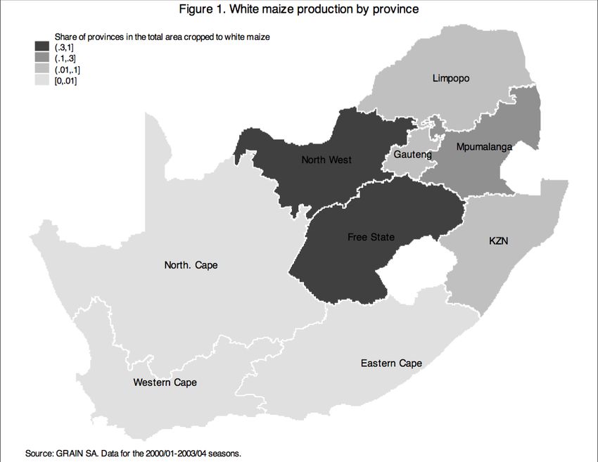
(Vicente-Serrano et al., 2010). More specifically, we apply this measure to the last growing

season. That is, we compute the mean index value for months from October to April at the

province level. Additionally, we also use the country average weighted by the share of each

province in the total area grown to white maize in order to capture the effect of local weather

shocks in the three provinces that provide the bulk of maize production, i.e. Free State, North

West and, to a lesser extent, Mpumalanga (Figure 1), on the total country supply. The data on

area grown and output per province come from GRAIN SA. Since each wave of the IES and

LCS surveys was conducted over 12 months, households interviewed in different months were

exposed to shocks in different growing seasons; in total, we can capture the variation in weather

conditions from eight different growing seasons. More importantly, during this period South

Africa experienced severe droughts, for example in the growing season 2007/08 and 2014/15. As

a robustness check, we also employ data from Agriculture Stress Index System (ASIS) by

FAO’s Global Information and Early Warning System (GIEWS).

 12

Descriptive Statistics

The descriptive statistics presented in Table 1 seem to support our arguments with respect to

weather shocks, food prices and food security in South Africa. On average, South African

households consumed 19 food items from 8 food groups over a reference period. Note, however,

that the reference period is different across survey waves, i.e. it is four weeks in the IES 2005/06

and LCS 2008/09, and two weeks in the IES 2010 and LCS 2014/15. The length of the reference

 13

period affects the dietary diversity measure (Ruel, 2003), and we expect that the longer the

period over which households are reporting their consumption, the greater the diversity of food

consumed. Indeed, the figures in Table 1 indicate that dietary diversity is definitely higher in

waves with four-week reference period. We control for this issue in all the regressions that

follow. Here, when we compare the mean dietary diversity between waves with the same

reference period, we can observe that both the number of food items and the number of food

groups consumed are lower in the LCS 2008/09 than in the IES 2005; and in the LCS 2014/15

than in the IES 2010/11.

 14

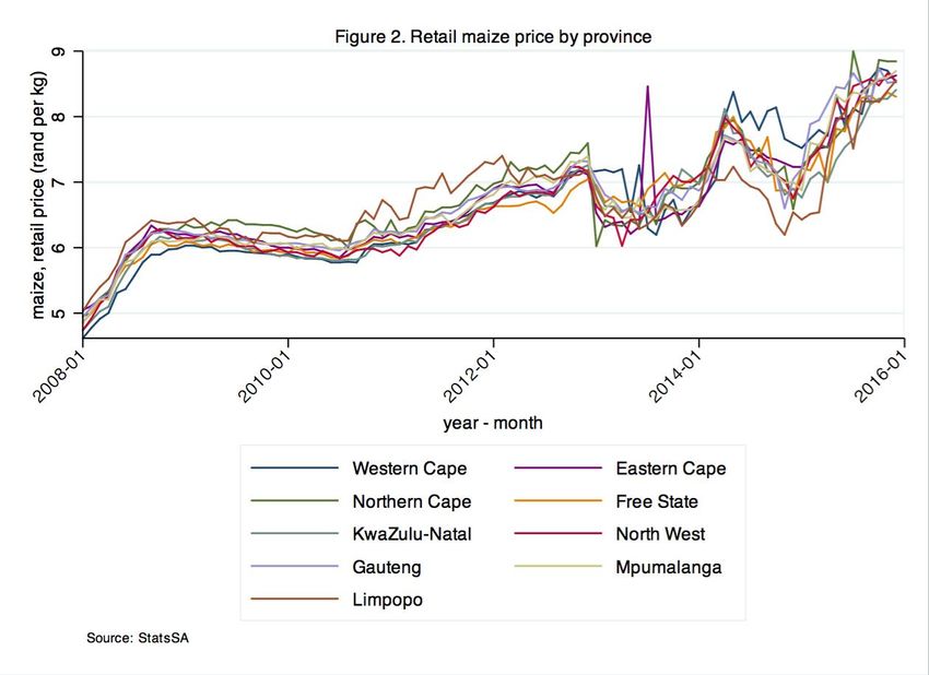
Not surprisingly, the dietary diversity decreases in years of weather stress and price spikes.

Indeed, the LCS 2008/09 and LCS 2014/15 households experienced much drier conditions, with

the SPEI index of -0.5 on average pointing to a moderate drought; however, the observed

drought intensity was much higher in certain provinces. The figures relative to ASI present a

similar picture, even though the increase in the agricultural stress in 2014/15 is not as spectacular

as in 2008/09. This, in turn, may result from the fact that while SPEI typically indicates

meteorological drought (Masih et al., 2014), ASI seeks to detect agricultural drought which takes

longer to develop, and indeed, ASI reached extremely high values only in 2016. Similarly, the

drought years coincide with the maize price spikes (Figure 2). This is especially visible in case of

the commodity price, which is not surprising taking into account asymmetry in the adjustment

process between commodity and retail prices (Vink & Kirsten, 2002). Interestingly, it is not only

the dietary diversity that decreases in the years of drought; food composition changes as well,

with, in particular, the increase in the share of cereals in the total consumption value. With

respect to the self-reported food security indicators, the lack of data in the IES 2005/06 and

IES2010 doesn’t allow for comparisons between years; however, the figures point to an overall

relatively high level of food insecurity in South Africa. More than 25 per cent of households

consider themselves to be food insecure, and around 20 per cent experienced any form of hunger

within past 12 months preceding the survey.

 15

Table 1. Descriptive statistics
 All waves IES 2005/06 LCS 2008/09 IES 2010/11 LCS 2014/15
Variable Mean St. dev. Mean St. dev. Mean St. dev. Mean St. dev. Mean St. dev.
Food security
Dietary diversity
Number of food items consumed 19.125 12.116 24.221 13.413 22.272 12.541 16.886 10.554 13.565 8.574
Household Dietary Diversity Score 8.257 2.906 9.455 2.689 9.099 2.586 7.578 2.819 7.007 2.800
Reference period 4 weeks 4 weeks 2 weeks 2 weeks
Food composition
Share of cereals in total cons. 0.294 0.177 0.261 0.153 0.334 0.168 0.280 0.177 0.297 0.197
Share of meat in total cons. 0.233 0.171 0.240 0.159 0.221 0.147 0.239 0.178 0.233 0.194
Share of diary in total cons. 0.094 0.094 0.089 0.083 0.092 0.080 0.097 0.100 0.100 0.110
Share of fruits and vegetables in total cons. 0.127 0.105 0.129 0.091 0.120 0.089 0.130 0.111 0.130 0.125
Self-reported food insecurity
Food insecure household 0.264 0.441 na. 0.273 0.445 na. 0.255 0.436
Hunger (adults) 0.209 0.406 na. 0.214 0.410 na. 0.203 0.402
Hunger (children) 0.183 0.387 na. 0.197 0.398 na. 0.168 0.374
Food variety lower than preferable 0.320 0.467 na. na. na. 0.320 0.467
Maize prices
Retail price, total country average (kg) 6.442 1.114 4.576 0.067 6.612 0.039 6.688 0.166 7.682 0.467
Commodity price (t) 1,711.762 590.143 1,090.076 180.102 1,657.200 154.153 1,505.351 229.179 2,556.119 436.457
Weather shocks
SPEI, total country weighted average -0.091 0.573 -0.256 0.030 -0.476 0.049 0.822 0.231 -0.517 0.075
ASI, total country weighted average 11.322 18.095 5.439 3.191 33.721 22.821 0.112 0.037 4.763 3.629
Household characteristics
Rural 0.381 0.486 0.439 0.496 0.382 0.486 0.357 0.479 0.354 0.478
Female head 0.442 0.497 0.441 0.496 0.444 0.497 0.436 0.496 0.447 0.497
Household size 3.860 2.508 4.019 2.683 3.888 2.496 3.752 2.351 3.803 2.515
African / Black 79.590 76.270 81.150 79.290 81.240
Coloured 10.980 12.740 10.050 10.750 10.650
Indian / Asian 1.750 1.650 1.600 1.850 1.890
White 7.680 9.350 7.200 8.110 6.210
Income, nominal 85,085.560 157,707.900 57,897.550 129,752.400 68,817.710 128,240.600 97,301.320 162,570.300 113,887.000 193,775.200
Expenditure, nominal 67,206.940 108,927.600 45,298.830 80,379.750 57,088.210 85,496.380 77,434.990 118,977.900 86,791.900 134,602.700
Food expenditure, nominal 11,469.090 11,923.650 7,492.015 8,175.455 12,952.610 12,399.060 11,837.260 12,316.920 13,075.880 12,969.140
Social welfare grant (exc. old age pension) 0.340 0.474 0.075 0.264 0.349 0.477 0.463 0.499 0.438 0.496
Own food production 0.168 0.374 na. 0.140 0.347 0.190 0.392 0.173 0.378
Income derived from own food production 0.011 0.106 na. 0.015 0.121 0.003 0.058 0.017 0.128
Number of observations 94,927 21,144 25,328 25,075 23,380

 16

Empirical Strategy

As noted earlier, typically, and particularly so in case of sub-Saharan Africa, the literature

analyzed the direct impact of weather shocks on food availability in case of own food production

by farmers. Here, we depart from this traditional approach and we model the link between

weather shocks and food security that acts specifically through food prices; therefore, this model

will be particularly relevant in contexts where a large share of households are net food buyers.

First, we assume that negative weather shocks affect agricultural productivity and lead to a

decrease in local food supply; this has previously been well established in the large literature and

does not require further attention in this paper. This reduction in food supply is then likely to

entail an increase in domestic food prices, and this effect might be especially pronounced in the

case of South Africa which is a net food exporter and where the international price transmission

mechanism is very limited (see below). In principle, the impact of weather shocks on prices

might be attenuated or exacerbated by the level of food stocks or grain reserves (Mirzabaev &

Tsegai, 2012), but because of data limitations, we are not able to control for this in our analysis.

Second, we expect the increase in food prices to negatively affect household food security, or,

more specifically, its access dimension. Of course, the impact of food prices on food security

might depend on the household food buyer / food seller position; however, in our dataset, around

17 per cent of households are involved in own food production activities, but only one per cent

derive any income from selling food produced on own plot, we can therefore safely assume that

households in our dataset are net food buyers. Note that in this model, we do not account for any

long-term secondary effects of weather shocks and food price increases on labour market

 17

conditions, and these might, indeed, be non-negligible3; however, we are not able to capture such

effects with the household survey data. In light of the assumptions discussed above, we employ

an instrumental variable model as in eq. (1):

 = ( , ) + (1)

 : ℎ 

where household’s i food security , measured as dietary diversity, depends on the level of

food prices in province j in year t, and where weather shocks do not affect food

security directly, but only through food prices. As a means of comparison, we also employ the

model with food prices and weather shocks at the country level; in this case the subscript j for

province should be removed. We also control for a set of household characteristics ,

including type of settlement (rural or urban), gender of household head, household size,

population group, own food production, and social grants. In order to represent the main

mechanism in our model, but also to take into account the endogeneity of food prices, we

instrument them with weather shocks. Technically, therefore, we capture the marginal

contribution of weather shocks to food prices, and use this variable to explain household food

security. Of course, weather shocks are only one of many factors influencing prices, and in

particular, we don’t account here for the long-term factors such as income levels, changes in

tastes and preferences or population growth.

3For example, the South African Agricultural Business Chamber reports on the commercial
agriculture sector clearly indicate that the employment is very responsive to seasonality,
weather and overall market conditions (AGBIZ, 2017).

 18

More importantly, we focus in this analysis specifically on the price of maize for several reasons.

First of all, white maize is a staple food in South Africa and therefore plays a central role in the

diets of the low-income households (Abidoye & Labuschagne, 2014; Altman et al., 2013).

Second, yellow maize is the single most important input in the dairy, pig, beef, and poultry

industries (Vink & Kirsten, 2002), and therefore, an increase in the price of maize implies that

the price of dairy and meat, major sources of protein in local diets, will increase accordingly.

Indeed, increase in the price of maize has been identified as the main driving force behind food

price inflation events (Vink & Kirsten, 2002; NAMC, 2003). Additionally, from the agricultural

production perspective, maize constitutes approximately 70 per cent of grain production and

covers 60 per cent of the country’s cropping area (Akpalu, Hassan, & Ringler, 2009), and

remains highly vulnerable to climate variability and climate change (Lobel et al., 2011).

What is more, since Southern Africa is the largest producer and consumer of white maize in the

world, the world price of white maize is largely determined by conditions in the South African

market (Vink & Kirsten, 2002). Further the international price transmission mechanism is

considered to be weak, with several studies suggesting that world maize prices have no

significant effect on South African maize prices (Minot, 2011; Kirsten, 2012), while others found

the threshold effect, where only large long-run deviations, such as oil price spike, are transmitted

to domestic market, but not the smaller changes (Abidoye and Labuschagne, 2014). The rand

exchange rate is, however, found to have an impact on the domestic food prices (Vink & Kirsten,

2002). In this context, we can expect that South African price of maize, but also prices of dairy

 19

and meat products, are shaped, to a large extent, by domestic conditions, and in particular, local

weather outcomes.4

Results

The main results of the 2SLS analysis are presented in Table 2. For sake of brevity, we do not

report the first-stage regressions output. The exogeneity of our instrument, i.e. weather shocks,

seems to be irrefutable, both intuitively and statistically; and its validity is confirmed in standard

tests (F-test, Anderson-Rubin Wald test5). Additionally, we verify these findings with the

conditional likelihood ratio (CLR) approach developed by Moreira (2003)6. Since we suspect

heteroscedasticity in our data, and indeed, the Breusch-Pagan test in the simple OLS regression7

supports this argument, we account for this issue in the following analyses. We present the

results for both measures of dietary diversity, i.e. the number of food items consumed and the

Household Dietary Diversity Score (HDDS). For ease of interpretation, we employ both

measures in logarithms; however, note that both are count variables, which might be particularly

meaningful in case of HDDS, and therefore, we also present the results for the Poisson

4 The remaining food groups, i.e. fresh products such as fruits and vegetables, are sourced
locally, and therefore their prices depend solely on local market conditions (Vink & Kirsten,
2002).
5 Note that our model is exactly identified, and therefore we cannot use other standard tests

such as Sargan-Hansen test.
6 Not reported here.
7 Not reported here.

 20

regression8 in Table A1 in the Annex. The main explanatory variable, i.e. price of maize, is also

used in logarithm.

In columns (1) – (2), we employ the total country average price of maize, and the country mean

seasonal SPEI averaged by the share of each province in the total area grown to white maize as

its instrument. The underlying assumption here is that local markets are spatially integrated and

therefore weather shocks in the last growing season, and in particular the shocks occurring in the

three provinces that are major producers of white maize, will affect prices in the whole country.

This might be plausible if we recall that South African households are net food buyers, and that

the share of big retail chains in total food sales is dominant and growing (see, for example,

Peyton, Moseley, & Battersby-Lennard, 2015).

An important limitation of such model, from a technical point of view, is that because of

multicollinearity, we cannot include dummy years and therefore control for possible structural

changes overs years. Keeping that in mind, and noting that the period under investigation follows

the sharp rise in commodity prices in 2006 and that beyond continued intensification of

production, does not appear to have had any other major change, we can, nevertheless, conclude

that, according to our expectations, food price shocks, entailed by weather shocks, do indeed

affect household food security, i.e. an increase in food prices by one per cent leads to a decrease

in the number of food items consumed by almost two per cent, or a decrease in the number of

food groups consumed, as reflected in the HDDS, by 0.8 per cent.

8More specifically, we employ ivpois method, which is a GMM estimator of Poisson regression
allowing for instrumental variables. Since the dependent variable is not over-dispersed and
does not have an excessive number of zeros, Poisson regression model seems appropriate here.

 21

On the other hand, if local markets are not well integrated, and if the small-scale or informal

trade plays an important role, then it is more appropriate to use the price and the weather data at

the province level9 as in columns (3) – (4)10. Johann Kirsten (personal communication, 2 October

2017) suggests that local food shortages occur even if the total country production registers a

surplus, and this, of course, have implications for local food prices; and Figure 2 shows that

while, globally, prices in South African provinces follow the same trend, they differ in the extent

of reaction to shocks, especially in recent years of severe drought. The results with respect to the

effect of price of maize on dietary diversity are overall confirmed, but the magnitude of the

coefficient increased substantially, especially in column (3) suggesting that indeed, this model is

more suitable. Importantly, in this model, year dummies are included which helps to isolate the

impact of weather shock and food prices on food security from structural factors. The results are

similar in terms of economic and statistical significance in the Poisson regression in Table A1.

The results with respect to control variables are generally in line with the literature, i.e. dietary

diversity is lower for rural households, while female-headed households demonstrate higher food

security. Important differences can be observed between different population groups; of course,

this might be as well related to the differences in wealth between these groups, and indeed,

wealthier households typically consume more diversified diets. Importantly, especially from the

policy perspective, social welfare grants, which cover a large population share in South Africa,

seem to improve household food security, even though, since they are targeted at low-income,

9More disaggregated data would be an optimal solution, but unfortunately, is not available.
10Note that price data at the province level is not available only for the IES 2005/06; therefore,
the number of observations decreases.

 22

and, potentially, food insecure, recipients, this variable might be flawed with endogeneity.

Finally, own food production, even though it might contribute only marginally to the total food

consumption, has a positive impact on household dietary diversity.

Additionally, we test if weather and price shocks, apart from affecting the number of food items

or food groups consumed, also influence household diets by changing the composition of food

consumption. We expect that as a result of food price increases, households, and especially the

poorest ones, will spend a greater share of their food expenditure on calorie-dense staples, i.e.

cereals, decreasing, at the same time, consumption of protein-rich but more expensive food

groups, such as meat or dairy. The figures in columns (5) – (8) confirm our hypothesis, with the

strongest effect observed for cereals; while the coefficient is insignificant in case of meat. On the

other hand, the magnitude of this effect is rather low; for example, an increase in food price by

one per cent entails an increase in the share of cereals in total consumption expenditure by 0.5

percentage point. This might be related to the fact that rather than substituting entire food groups,

household resort to brand switching, i.e. choosing lower quality products than usually. Such

effect was, for example, observed in a small-scale study presented by NAMC (2003); in our

study, we are not able to detect this kind of substitution due to the fact that our data on food

consumption is aggregated at the COICOP level.

 23

Table 2. Weather shocks, food prices and food security
 Dietary diversity Food composition

 Number of food Household Number of food Household
 Fruits and
 items consumed Dietary Diveristy items consumed Dietary Diveristy Cereals Dairy Meat
 vegetables
 (log) Score (log) (log) Score (log)

 2SLS 2SLS 2SLS 2SLS 2SLS 2SLS 2SLS 2SLS
 (1) (2) (3) (4) (5) (6) (7) (8)

Maize price, total country (log) -1.867*** -0.831***
 -0.0423 (0.0294)
Maize price, province (log) -2.506*** -0.881** 0.496*** -0.316*** 0.0766 0.228**
 (0.585) (0.382) (0.158) (0.0961) (0.168) (0.107)
Rural -0.0844*** -0.0622*** -0.0917*** -0.0643*** 0.0290*** -0.0104*** -0.0226*** 0.000495
 (0.00632) (0.00439) (0.00688) (0.00469) (0.00200) (0.00111) (0.00196) (0.00130)
Housheold size 0.0473*** 0.0246*** 0.0476*** 0.0247*** 0.00713*** -0.00203*** -0.00270*** -0.00191***
 (0.00101) (0.000669) (0.00103) (0.000672) (0.000302) (0.000153) (0.000282) (0.000183)
Black (reference group)

Coloured 0.0636*** 0.0301*** 0.0634*** 0.0304*** -0.0223*** 0.00127 0.0218*** -0.00555***
 (0.00894) (0.00561) (0.00905) (0.00564) (0.00227) (0.00140) (0.00266) (0.00146)
Indian / Asian -0.0201 -0.00717 -0.0155 -0.00546 -0.0261*** 0.0317*** -0.0332*** 0.0153***
 (0.0180) (0.0118) (0.0180) (0.0118) (0.00468) (0.00312) (0.00543) (0.00324)
White 0.207*** 0.0905*** 0.204*** 0.0894*** -0.0695*** 0.0346*** -0.0288*** 0.0341***
 (0.0104) (0.00640) (0.0105) (0.00644) (0.00230) (0.00176) (0.00288) (0.00181)
Female household head 0.0224*** 0.0177*** 0.0223*** 0.0176*** 0.00638*** 0.000189 -0.0171*** 0.0125***
 (0.00451) (0.00305) (0.00456) (0.00306) (0.00131) (0.000731) (0.00130) (0.000853)
Wealth index 0.0884*** 0.0394*** 0.0869*** 0.0389*** -0.0162*** 0.00658*** 0.0127*** -0.00189***
 (0.00163) (0.00109) (0.00169) (0.00113) (0.000489) (0.000264) (0.000471) (0.000315)
Social welfare grant 0.0302*** 0.0260*** 0.0313*** 0.0265*** 0.00335** -0.00295*** -0.00203 0.00176*
 (0.00514) (0.00345) (0.00521) (0.00347) (0.00152) (0.000822) (0.00148) (0.000959)
Own food production 0.0244*** 0.0110** 0.0240*** 0.0112** 0.00676*** -0.00370*** -0.0105*** 0.00634***
 (0.00643) (0.00444) (0.00652) (0.00446) (0.00203) (0.00103) (0.00184) (0.00129)
Constant 5.984*** 3.389*** 7.538*** 3.553*** -0.924** 0.847*** 0.104 -0.371
 (0.0869) (0.0599) (1.331) (0.869) (0.359) (0.219) (0.382) (0.244)
Province dummy Yes Yes Yes Yes Yes Yes Yes Yes
Year dummy No No Yes Yes Yes Yes Yes Yes

Observations 72,927 72,980 72,927 72,980 72,927 72,927 72,927 72,927
R-squared 0.272 0.190 0.256 0.186 0.149 0.057 0.060 0.012

Notes: Instrumented: logarithm of maize price. Instrument: SPEI12. First-stage regressions omitted. All regressions control for the survey reference period. Robust standard errors in parentheses. *** p

Table 3. Dietary diversity by wealth quartile
 1st quartile 2nd quartile 3rd quartile 4th quartile
 Mean St. dev. Mean St. dev. Mean St. dev. Mean St. dev.

Number of food items consumed 14.57 8.53 16.30 9.21 19.48 10.56 26.16 15.49
Household Dietary Diveristy Score 7.37 2.79 7.77 2.74 8.45 2.73 9.43 2.93

Number of observations 23732 23779 23702 23714

The figures in Table 2 suggest that wealth affect household food security, which corresponds to

our expectations and to the findings in the literature. Indeed, simple tabulations show that the

dietary diversity differs substantially between wealth groups (Table 3), i.e. the first quartile

reports 15 food items and 7 food groups on average, whereas the fourth 26 food items and 9 food

groups respectively. More importantly, the standard deviation, especially in case of the number

of food items consumed, increases with wealth, too; we might therefore expect that different

wealth groups will respond differently to a price shock. Table 4 presents the results of

regressions by wealth quartile, and these seem to be compatible with our expectations. In terms

of the number of food items consumed, the food price shock turns out significant only for the

two middle quartiles of wealth distribution, but is insignificant for the poorest and for the richest

households. This is not surprising; the poorest households, almost by definition, are the most

food insecure and consume the least diversified diets limited to the necessary minimum, and, as

result, they have little scope to decrease their dietary diversity even further as a response to food

price shocks. The richest households, on the other hand, are not financially constrained and

therefore, food price shocks do not affect their food consumption patterns. More importantly,

with respect to HDDS, only households from the second quartile adjust their food consumption

to food price shocks; and this result is probably even more meaningful taking into account that

contrary to the simple count of food items, HDDS reflects better the distribution of food groups,

 25

and consequently, macro and micronutrient, in the food basket. These findings are in line with

the literature pointing to the fact that the poor are at a higher risk of food insecurity.

 Table 4. Weather shocks, food prices and food security by wealth quartiles
 Number of food items consumed (log) Household Dietary Diveristy Score (log)
 1st quartile 2nd quartile 3rd quartile 4th quartile 1st quartile 2nd quartile 3rd quartile 4th quartile
 2SLS 2SLS 2SLS 2SLS 2SLS 2SLS 2SLS 2SLS
 (1) (2) (3) (4) (5) (6) (7) (8)

Maize price, province (log) -1.372 -2.552*** -3.696** 31.24 -0.482 -1.321*** -0.983 22.13
 (0.854) (0.581) (1.538) (64.84) (0.602) (0.395) (0.988) (42.44)
Rural -0.113*** -0.0751*** -0.0867*** 0.206 -0.0794*** -0.0512*** -0.0574*** 0.150
 (0.0121) (0.0119) (0.0154) (0.621) (0.00874) (0.00821) (0.0101) (0.407)
Housheold size 0.0511*** 0.0410*** 0.0428*** 0.0475*** 0.0291*** 0.0216*** 0.0211*** 0.0209***
 (0.00190) (0.00200) (0.00205) (0.00689) (0.00129) (0.00136) (0.00133) (0.00500)
Black (reference group)

Coloured 0.0245 0.0224 0.0523*** 0.107 0.0136 0.00163 0.0192* 0.0664
 (0.0279) (0.0220) (0.0165) (0.0672) (0.0193) (0.0143) (0.0103) (0.0454)
Indian / Asian 0.302*** 0.188*** -0.0116 -0.0972 0.129 0.113*** 0.00421 -0.0596
 (0.0968) (0.0626) (0.0380) (0.144) (0.110) (0.0409) (0.0253) (0.0954)
White 0.127 0.176*** 0.0754** 0.258** -0.0139 0.0624 0.0201 0.126*
 (0.125) (0.0656) (0.0373) (0.104) (0.0851) (0.0411) (0.0233) (0.0686)
Female household head 0.0345*** 0.0320*** 0.0234*** -0.0206 0.0185*** 0.0179*** 0.0218*** -0.00197
 (0.00926) (0.00902) (0.00876) (0.0311) (0.00666) (0.00623) (0.00572) (0.0208)
Social welfare grant 0.0819*** 0.0736*** 0.0357*** -0.0784*** 0.0523*** 0.0492*** 0.0275*** -0.0305
 (0.0107) (0.0104) (0.00967) (0.0304) (0.00762) (0.00714) (0.00620) (0.0211)
Own food production 0.0415*** 0.00455 0.0109 0.0589 0.0227*** -0.00298 0.00423 0.0373
 (0.0109) (0.0118) (0.0142) (0.0733) (0.00776) (0.00821) (0.00939) (0.0515)

Constant 4.668** 7.588*** 10.34*** -69.87 2.459* 4.536*** 3.835* -49.24
 (1.925) (1.314) (3.515) (149.3) (1.357) (0.894) (2.257) (97.72)
Province dummy Yes Yes Yes Yes Yes Yes Yes Yes
Year dummy Yes Yes Yes Yes Yes Yes Yes Yes

Observations 18,064 18,289 18,283 18,291 18,104 18,297 18,287 18,292
R-squared 0.209 0.158 0.140 -3.336 0.160 0.125 0.143 -4.971
Notes: Instrumented: logarithm of maize price. Instrument: SPEI12. First-stage regressions omitted. All regressions control for the survey
reference period. Wealth quartiles based on asset-based index based on the polychoric principal component analysis (Kolenikov & Angeles,
2004). Robust standard errors in parentheses. *** p

Table 5. The results point, however, to the contrary and show that households involved in

farming activities are actually more vulnerable to weather and food price shocks, with the

magnitude of the coefficient more than three times higher. This does not come as a surprise when

we take into account the complexity of livelihoods strategies of the poorest households. Indeed,

typically only the poorest households resort to subsistence farming, i.e. the incidence of

subsistence farming activities is 25 per cent for the first wealth quartile and less than 7 per cent

for the fourth quartile. Whereas this strategy proves overall helpful and, by decreasing the

dependence on food purchases, albeit marginally, it increases household food security, as shown

in Table 4, it can exacerbate household vulnerability to weather shocks. We can hypothesize that

a weather shock brings about crop failure; as a consequence, households will have to substitute

food from own production with food purchases; however, they will face higher food prices

resulting from the aggregate food shortage. Indeed, the extent of this effect is much higher when

we employ the country level measures of food price and weather shock.11 Additionally, with

reference to Hendriks (2003), we control for the income derived from own food production in

columns (2) and (5); however, we do not find any significant effect, which is very likely taking

into account the low number of households reporting such income.

11 Results not reported here.

 27

Table 5. Weather shocks, food prices and food security: role of own food production
 Number of food items consumed (log) Household Dietary Diveristy Score (log)
 No food No food
 Own food production Own food production
 production production
 2SLS 2SLS 2SLS 2SLS 2SLS 2SLS
 (1) (2) (3) (4) (5) (6)

Maize price, province (log) -5.356*** -5.374*** -1.737** -2.225*** -2.227*** -0.432
 (0.999) (1.000) (0.734) (0.656) (0.657) (0.477)
Rural -0.0799*** -0.0801*** -0.0912*** -0.0527*** -0.0527*** -0.0642***
 (0.0164) (0.0165) (0.00791) (0.0108) (0.0108) (0.00540)
Housheold size 0.0446*** 0.0446*** 0.0482*** 0.0232*** 0.0232*** 0.0250***
 (0.00215) (0.00215) (0.00119) (0.00140) (0.00140) (0.000773)
Black (reference group)

Coloured -0.0171 -0.0170 0.0627*** -0.00123 -0.00122 0.0294***
 (0.0481) (0.0481) (0.00919) (0.0287) (0.0287) (0.00576)
Indian / Asian 0.150 0.150 -0.0184 0.0745 0.0745 -0.00604
 (0.150) (0.151) (0.0182) (0.0862) (0.0863) (0.0120)
White 0.265*** 0.263*** 0.197*** 0.127*** 0.127*** 0.0857***
 (0.0409) (0.0410) (0.0110) (0.0240) (0.0240) (0.00675)
Female household head 0.0304*** 0.0307*** 0.0203*** 0.0144* 0.0144* 0.0181***
 (0.0114) (0.0114) (0.00501) (0.00753) (0.00753) (0.00337)
Wealth index 0.0726*** 0.0725*** 0.0896*** 0.0324*** 0.0324*** 0.0402***
 (0.00417) (0.00417) (0.00189) (0.00272) (0.00272) (0.00127)
Social welfare grant 0.0557*** 0.0559*** 0.0263*** 0.0346*** 0.0346*** 0.0247***
 (0.0131) (0.0131) (0.00570) (0.00873) (0.00874) (0.00378)
Income from own food production 0.0204 0.00256
 (0.0238) (0.0159)

Constant 13.75*** 13.78*** 5.812*** 6.474*** 6.479*** 2.540**
 (2.224) (2.226) (1.676) (1.460) (1.461) (1.089)
Province dummy Yes Yes Yes Yes Yes Yes
Year dummy Yes Yes Yes Yes Yes Yes

Observations 12,307 12,307 60,620 12,311 12,311 60,669
R-squared 0.105 0.104 0.275 0.110 0.110 0.196
Notes: Instrumented: logarithm of maize price. Instrument: SPEI12. First-stage regressions omitted. All regressions control for
the survey reference period. Robust standard errors in parentheses. *** p

adequate, or more than adequate), the experience of hunger in case of children as well as adult

household members (never, seldom, often, or always). We use these questions to construct

dummies for food insecurity (equal to one if a household reports less than adequate food

consumption) as well as child and adult hunger (equal to one if children or adults, respectively,

within a household were reported to seldom, often, or always go hungry). Additionally, the LCS

2014/15 provides data on household coping strategies in case of insufficient availability of food,

including reduction in food variety. We apply an instrumental variable probit model to estimate

if the food price, instrumented with weather shock, affect the probability of these measure of

food insecurity measures being reported. Keeping in mind that the sample size is now reduced by

half due to the lack of the data in the IES surveys, this is, nevertheless, a valuable way to

compare the official indicators of food security with individual perceptions.

The figures in Table 6 confirm our main findings. In particular, weather shocks and food prices

significantly affect household food security status; i.e. a one per cent increase in food prices

increases the probability of a household being food insecure by around 0.7 percentage point12,

and similar effect is found for the remaining measures of food insecurity, even though the

magnitude of the effect is much lower in case of child hunger. Most notably, a price increase

induced by weather shock increases the probability of a household reporting lower food

diversity, and this result offers relatively best comparability with our main findings. Regarding

the control variables, previous results are confirmed with respect to the impact of wealth or

population group, but they are less precise in case of own food production or rural dummy.

These discrepancies might, however, result from the contextual factors affecting individual

12Remember that food prices are employed in logarithm, therefore, the marginal effect
reported in Table 6 refers to a change in food prices by one log.

 29

perceptions and reference groups. Additionally, we checked the robustness of our main findings

by employing the commodity price of maize as the principal explanatory variable and second,

and by using the Agricultural Stress Index (ASI) and, alternatively, the drought dummy from

EM-DAT dataset, as the instrument for food prices13. The results for commodity price are similar

to the ones for the retail price at the country level, even though the magnitude is smaller which is

not surprising taking into account the asymmetric adjustment between commodity and retail

prices (Vink & Kirsten, 2002). On the other hand, the results for ASI produce higher estimates of

the effect of food price on dietary diversity, which might be due to the fact that ASI captures

longer-term changes in weather patterns.

13 Results not reported here.

 30

Table 6. Weather shocks, food prices and self-reported measures of food insecurity
 Food insecure Hunger Lower food
 Hunger (adults)
 household (children) variety
 IV probit IV probit IV probit IV probit
 (1) (2) (3) (4)

Maize price, province (log) 1.257*** 1.086*** 0.793*** 1.593***
 (0.234) (0.226) (0.221) (0.212)
Rural -0.0251*** -0.0623*** -0.0584*** -0.0487***
 (0.00499) (0.00458) (0.00532) (0.00930)
Housheold size 0.0119*** 0.0115*** 0.0139*** 0.0205***
 (0.000760) (0.000697) (0.000797) (0.00116)
Black (reference group)

Coloured -0.0504*** -0.0289*** -0.0404*** -0.0352***
 (0.00668) (0.00637) (0.00686) (0.0103)
Indian / Asian -0.0941*** -0.1000*** -0.116*** -0.100***
 (0.0159) (0.0142) (0.0161) (0.0233)
White -0.156*** -0.143*** -0.120*** -0.149***
 (0.00831) (0.00747) (0.0102) (0.0129)
Female household head 0.0214*** 0.0151*** 0.0389*** 0.0296***
 (0.00386) (0.00362) (0.00412) (0.00574)
Wealth index -0.0657*** -0.0619*** -0.0517*** -0.0751***
 (0.00139) (0.00121) (0.00134) (0.00238)
Income from own food production -0.0146*** 0.0189*** 0.0268*** 0.0626***
 (0.00546) (0.00531) (0.00576) (0.00818)

Observations 47,786 46,833 33,118 23,074
Notes: Instrumented: logarithm of maize price. Instrument: SPEI12. Results presented in terms of the average
marginal effects. First-stage regressions omitted. All regressions control for the survey reference period. Robust
standard errors in parentheses. *** p