On the Design of an Efficient Cardiac Health Monitoring System Through Combined Analysis of ECG and SCG Signals - MDPI
←
→
Page content transcription
If your browser does not render page correctly, please read the page content below
sensors
Article
On the Design of an Efficient Cardiac Health
Monitoring System Through Combined
Analysis of ECG and SCG Signals
Prasan Kumar Sahoo 1,4          ID
                                     , Hiren Kumar Thakkar 1 , Wen-Yen Lin 2,4 , Po-Cheng Chang 4 and
Ming-Yih Lee 3,4, * ID
 1   Department of Computer Science and Information Engineering, Chang Gung University, Guishan 33302,
     Taiwan; pksahoo@mail.cgu.edu.tw (P.K.S.); D0221015@cgu.edu.tw (H.K.T.)
 2   Department of Electrical Engineering and Center for Biomedical Engineering/College of Engineering,
     Chang Gung University, Guishan 33302, Taiwan; wylin@mail.cgu.edu.tw
 3   Graduate Institute of Medical Mechatronics, Center for Biomedical Engineering, Chang Gung University,
     Guishan 33302, Taiwan
 4   Division of Cardiology, Department of Internal Medicine, Chang Gung Memorial Hospital, Linkou 33305,
     Taiwan; pccbrian@gmail.com
 *   Correspondence: leemiy@mail.cgu.edu.tw; Tel.: +886-3-211-8800 (ext. 5340)

 Received: 30 November 2017; Accepted: 24 January 2018; Published: 28 January 2018

 Abstract: Cardiovascular disease (CVD) is a major public concern and socioeconomic problem across
 the globe. The popular high-end cardiac health monitoring systems such as magnetic resonance
 imaging (MRI), computerized tomography scan (CT scan), and echocardiography (Echo) are highly
 expensive and do not support long-term continuous monitoring of patients without disrupting
 their activities of daily living (ADL). In this paper, the continuous and non-invasive cardiac health
 monitoring using unobtrusive sensors is explored aiming to provide a feasible and low-cost alternative
 to foresee possible cardiac anomalies in an early stage. It is learned that cardiac health monitoring
 based on sole usage of electrocardiogram (ECG) signals may not provide powerful insights as ECG
 provides shallow information on various cardiac activities in the form of electrical impulses only.
 Hence, a novel low-cost, non-invasive seismocardiogram (SCG) signal along with ECG signals are
 jointly investigated for the robust cardiac health monitoring. For this purpose, the in-laboratory
 data collection model is designed for simultaneous acquisition of ECG and SCG signals followed by
 mechanisms for the automatic delineation of relevant feature points in acquired ECG and SCG signals.
 In addition, separate feature points based novel approach is adopted to distinguish between normal
 and abnormal morphology in each ECG and SCG cardiac cycle. Finally, a combined analysis of ECG
 and SCG is carried out by designing a Naïve Bayes conditional probability model. Experiments on
 Institutional Review Board (IRB) approved licensed ECG/SCG signals acquired from real subjects
 containing 12,000 cardiac cycles show that the proposed feature point delineation mechanisms and
 abnormal morphology detection methods consistently perform well and give promising results. In
 addition, experimental results show that the combined analysis of ECG and SCG signals provide
 more reliable cardiac health monitoring compared to the standalone use of ECG and SCG.

 Keywords: cardiovascular disease (CVD); electrocardiogram (ECG); seismocardiogram (SCG);
 cardiac anomalies

1. Introduction
     Recent advancements in sensor technology have made it possible to use low-powered, inexpensive
sensor-based devices to monitor various physiological parameters related to human health such as
heart rate, blood pressure, body temperature etc., [1,2]. Numerous applications are becoming reality in

Sensors 2018, 18, 379; doi:10.3390/s18020379                                    www.mdpi.com/journal/sensors
Sensors 2018, 18, 379                                                                                 2 of 28

the light of wearable sensor technology such as diet monitoring, drug monitoring, activity detection,
cardiac health monitoring, etc. [3]. Among the envisioned applications, designing a robust cardiac
health monitoring system to capture early signs of gradually developing cardiac anomalies using
low-cost wearable body sensors is a growing interest among medical and research communities as it
has serious consequences on human health. According to World Health Organization [4], CVD is the
leading cause of death in people across all age groups. Moreover, the recent report of the American
Heart Association [5] reveals that as high as 30% annual mortality rate is observed due to CVD in
the United States and Canada. Under such circumstances, there is a growing need for a reliable and
low-cost system that potentially aids in robust cardiac health monitoring.
       Several cardiac events take place during successive heartbeats such as opening and closing
of the heart valves, blood flow into vessels, contraction–relaxation of ventricular walls, etc. For a
healthy person, cardiac events unfold at regular intervals in a predefined order. However, cardiac
abnormalities such as myocardial ischemia, infarction, arrhythmias, etc., hinder the normal functioning
of cardiac events leading to CVD. Such cardiac abnormalities may result in dizziness, nausea, chest
pain, etc., which may lead to severe consequences such as heart attacks if not detected and taken care
of in an early stage. In many instances, the irregular heartbeats known as ectopic heartbeats appear
intermittently without showing any serious symptoms. Such ectopic heartbeats are becoming quite
common among healthy population and are often getting unnoticed.
       Nowadays, several clinical practices are used to monitor the cardiac abnormalities such as ECG,
magnetic resonance imaging (MRI), computerized tomography scan (CT scan), Echocardiography
(Echo), Nuclear myocardial perfusion scan etc., [6]. Among the mentioned clinical practices, ECG is a
well-established and widely adopted practice to monitor physiological activities of the heart. However,
ECG provides shallow information on the functioning of various cardiac events. Moreover, a study
conducted in [7] recommends that sole use of ECG is not reliable for the diagnosis of serious cardiac
abnormalities. On the other hand, MRI, CT scan, and Echo are reliable practices over ECG, but they are
highly expensive, time-consuming, and labor-intensive, which often require expertise to carry out [6].
       Different from the aforementioned clinical practices, non-invasive acquisition of cardiac signals
such as seismocardiogram (SCG) and ballistocardiogram (BCG) are also potential low-cost alternatives
to monitor cardiac mechanical activities. SCG is an accelerometer sensor based modality that can record
ultra-low-frequency vibrations of cardiac cycle mechanics along with timings of corresponding cardiac
events [8]. Although BCG and SCG can record cardiac mechanical activities, diagnosis based on them
is still in the premature stage to be considered for clinical practices. However, recent literature [6,8–11]
show growing confidence on the applicability of SCG in clinical practices over BCG. Moreover, SCG is
a noninvasive as well as an inexpensive accelerometer-based cardiac recording method, which can
easily be carried out using wearable sensors. Hence, in this proposal, SCG is explored as an additional
measure along with the ECG to design a robust cardiac health monitoring system.
       In past, it was difficult to gather a huge amount of continuous cardiac data such as ECG and SCG
to carry out comprehensive analysis. However, recent advancements in wearable technology have
made it possible to collect cardiac data in an easy and affordable manner via wearable sensors for the
longer duration. Although most cardiac abnormalities often appear only intermittently, they need to
be registered, tracked and analyzed thoroughly as time goes by. This encourages us to design an early
warning system, where continuously generated cardiac data are analyzed thoroughly to capture early
signs of cardiac abnormal behavior.
       The rest of the paper is organized as follows. Section 2 describes the related works followed by
motivation and goals of the paper. The system model is presented in Section 3. Cardiological data
analysis is described in Section 4. Performance evaluation is carried out in Section 5. Results and
discussions are made in Section 6. Concluding remarks and future works are discussed in Section 7.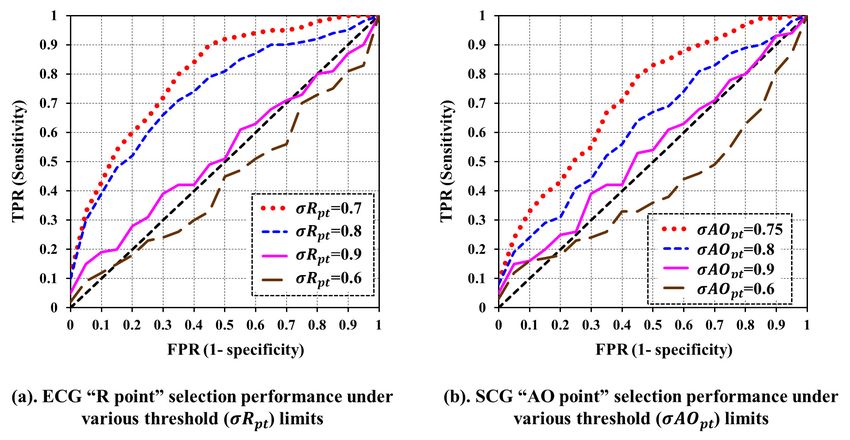
Sensors 2018, 18, 379                                                                              3 of 28

2. Related Works
      In the past, several efforts are made to remotely monitor various physiological parameters of
a user using affordable body sensors in a continuous manner. The LifeGuard [12] is one of the early
efforts that monitors electrocardiogram, heart rate, respiration rate, temperature and blood pressure
to alert the users. The LifeGuard equipped system transfers the health parameters to the base station
via Bluetooth-enabled cell phone and raises the buzzer alarm, whenever abnormalities are observed.
Similarly, in [13], ECG based body networks are proposed that raise an alarm if a heart attack is
detected. However, many times due to bad signal quality or intense physical activities by a user,
systems may raise false alarms under normal circumstances as well. In [14], a false arrhythmia alarm
reduction framework is proposed using machine learning. In [15], ECG-based automatic recognition
of arrhythmias is proposed for the diagnosis of heart diseases. Usually, remote monitoring of a person
becomes a challenging job, if a person is engaged in activities such as motor racing, cycling, car racing
and on field military service. The Smart Helmet is specifically designed to address the aforementioned
challenges and proposes a bio-sensors equipped embedded helmet to monitor ECG and respiration of
a user in an uninterrupted manner [16].
      The another recent effort to remotely monitor cardiovascular and respiratory variables is a
mobile healthcare platform PlaIMoS [17]. The conceived PlaIMoS architectural platform typically
deals with data collection, communication, analysis and visualization of various healthcare settings.
In continuously generated large data sets of ECG patterns, it is highly challenging to visualize cardiac
health information aggregated over the period of time. Under such circumstances, easy-to-interpret
visualization facility on cardiac health information is highly desirable to distinguish between healthy
and abnormal cardiac settings. The ECG Clock Generator [18] is an attempt to provide visualization
facility of cardiac activities accumulated over the period of time using ECG patterns.
      In addition to ECG, in recent times, seismocardiogram (SCG) signals are also used to monitor the
vital cardiac health parameters. In [19], authors have designed seismocardiography using tri-axial
accelerometer embedded with electrocardiogram. Recently, Di Rienzo et al. [20] have designed
accelerometer sensors based smart garment to record as well as monitor ECG, SCG, and respiratory
variables of an ambulant subject out-of-laboratory setting. SCG also has potential clinical applications
such as real-time heart rate monitoring [21] and left ventricular health monitoring [22] from wearable
SCG measurements.
      The raw SCG signals are less informative unless specific peaks are identified and correlated
with underlying cardiac activities. A typical SCG cardiac cycle includes a set of nine relevant peaks,
also called as feature points such as atrial systole AS, closing of mitral valve MC, opening of aortic
valve AO, rapid systolic ejection RE, closing of aortic valve AC, opening of mitral valve MO, rapid
diastolic filling RF, isovolumic movement I M, and isovolumic contraction IC. Various hemodynamic
parameters can be estimated using SCG feature points. For example, in [23] systolic time intervals
such as pre-ejection time (PEP), left ventricle ejection time (LVET), and electromechanical systole (QS2)
are estimated by identifying SCG feature points AO, AC, I M, MO, and MC. Similarly, in [8], cardiac
time intervals PEP, LVET, systolic time (SYS), and diastolic time (DIA) are estimated by identifying
relevant SCG feature points.
      In recent years, SCG shows numerous applications in real-time continuous health monitoring.
For example, SCG is employed for the detection of respiratory phases in [9] such as inhale or exhale,
which subsequently enable the estimation of systolic time intervals. In [11], the heart condition
is estimated from the learned morphology of seismocardiography. In [24], SCG based automated
detection of atrial fibrillation is demonstrated. In [25], a comparative study on pulse transit time
measurement using seismocardiography, photoplethysmography and acoustic recordings is carried
out. In [10], a cardiac early warning system using wearable ECG and SCG signals is introduced. In [6],
a multichannel SCG is employed and six location-specific feature points are identified in addition to
nine SCG feature points described previously.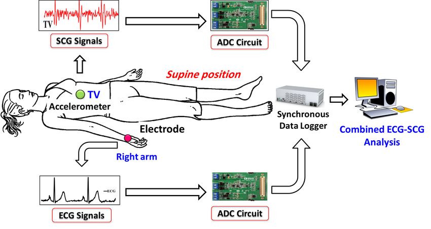
Sensors 2018, 18, 379                                                                              4 of 28

       To the best of our knowledge, the state-of-art recent studies [6,8,23] exclusively focus on
separate or combined annotation of ECG and SCG or focus on the annotation based disease-specific
cardiac function monitoring [9,24]. However, mere annotation of morphologies may not provide the
powerful insight unless the comprehensive theoretical analysis is explored. Since ECG and SCG are
pseudo-accurate in nature, their exclusive usage for the cardiac health monitoring limits the scope of
the improvement. It is known that ECG signals represent only cardiac electrical activities and all heart
problems cannot be detected by analyzing these ECG signals. For example, a common heart disorder
known as angina may not usually appear in routine ECG. In addition, vulnerable plaque deposition,
which is mainly responsible for asymptomatic blockages in heart arteries, is difficult to capture by
ECG and requires detailed investigation and tests. The Seismocardiogram (SCG) can be employed
to complement the ECG as SCG represents the cardiac mechanical activities and provides in-depth
meaningful insights of the mechanical functioning of the heart. However, SCG has also few limitations
such as lack of well studied features to determine the heart conditions such as hypertensive heart
disease. Hence, feature points based beat-by-beat combined analysis of ECG and SCG is expected to
bring additional information to carry out the detail analysis for continuous cardiac health monitoring.
It is likely that joint analysis of ECG and SCG can complement to each other to produce more reliable
outcomes. The combined analysis of ECG and SCG is beneficial as the outcome of each heartbeat is
validated based on the combined knowledge of the cardiac electrical and mechanical activities.

Motivation and Goals
      It is increasingly becoming important to record, monitor and investigate the intermittent cardiac
anomalies those appear due to the unhealthy lifestyle of people leading to CVD. Usually, cardiac
anomalies may occur only intermittently and they go completely unnoticed leading to a sudden death
of a cardiac patient. Moreover, ECG signals of cardiac patients also stay entirely normal on regular
basis except during those intermittent cardiac anomalies. Under such circumstances, it is highly
challenging to foresee potential cardiac health problems in the early stage using traditional in-hospital
ECG based diagnosis.
      To capture intermittent cardiac anomalies, various cardiac health parameters need to be recorded
and monitored for the longer duration of time, which can be accomplished via wearable ECG and
SCG sensors. However, raw ECG and SCG signals are less informative unless signals are properly
annotated and thoroughly investigated beat by beat. The manual annotation of feature points is a
tedious, cumbersome and time-consuming process. In addition, the manual annotation is not a viable
approach to design a continuous cardiac health monitoring system. Hence, the computer-assisted
automatic annotation of ECG and SCG is highly essential. Additionally, feature points based cardiac
health monitoring methods are needed to distinguish the morphology of any cardiac cycle between
normal and abnormal. In the proposed study, by use of phrase anomalies, we mean the unusual
morphology of ECG and SCG in terms of uncommon recording of an amplitude of peaks, and duration
of waves, segments, and intervals. It is to be noted that the mere presence of uncommon recordings in
a single cardiac cycle does not mean the cardiac anomalies. For this reason, the set of cardiac cycles is
needed to be monitored to help capture developing trends for the cardiac early warnings.
      Since cardiac health monitoring is a very broad area, we limit the scope of our investigation only
to jointly monitor the normal vs. abnormal behavior of cardiac cycles in simultaneous ECG and SCG
recordings. The main objective is to present the viability of joint investigation of ECG and SCG for
long-term cardiac health monitoring. In the future, the study can be extended to accommodate the
urgency of the abnormality. The goals of our study are listed as follows:

1.    Design a body sensor network to collect the simultaneous ECG and SCG signals;
2.    Design automatic feature point delineation algorithm for annotation of ECG and
      SCG signals;
3.    Design abnormal morphology detection method for ECG signals;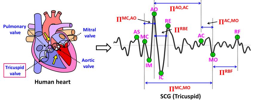
Sensors 2018, 18, 379                                                                               5 of 28

4.    Design abnormal morphology detection method for SCG signals;
5.    Design combined analysis model for ECG and SCG signals.

3. System Model
      The architectural view of the proposed ECG and SCG data collection model is shown in Figure 1.
For SCG data collection, an SCG sensing module is placed at a valvular auscultation site called a
Tricuspid valve TV, and ECG data collection is carried out placing an ECG sensing module (e.g.,
electrode) at the right arm as shown in Figure 1. The high quality disposable electrode H135SG
Covidien from Bio-Medical Instruments (Clinton Township, MI, USA) [26] is used as an ECG sensing
module. The accelerometer sensor LIS331DLH from STMicroelectronics (Geneva, Switzerland) [27] is
used as a core component of SCG sensing module. The sensing ability, sensing range and gravitational
force sensitivity of SCG sensing module is set to 0.5 Hz to 1 kHz, +2 g to –2 g, and 1 mg, respectively.
The band pass filter with frequency 0.5 Hz–50 Hz is applied analogically to get the required ECG and
SCG signals at sampling frequency of 1000 Hz. The microcontroller system ADuC7020 from Analog
Devices Inc. (Cambridge, MA, USA) [28] is used for the communication from ECG/SCG sensing
modules to Analog-to-Digital convert (ADC) circuit and the PowerLab 16/35 from AD Instruments
(Dunedin, New Zealand) [29] is used as the synchronous data logger, which further amplifies and
filters the concurrent signals. The class of nonlinear filters also known as filter bank presented in [30]
is employed for the noise reduction and baseline wander removal with minimal signal distortion. It is
reported that the nonlinear filters are expected to perform better than other baseline wander removal
methods such as adaptive filters, moving average filters, etc. [30].

                        Figure 1. Architectural view of ECG/SCG data collection model.

     The SCG signals acquired from Tricuspid valve and lead I ECG signals are used for the combined
analysis. The conventional Tricuspid valve site is chosen as the interventricular septum is located
beneath the Tricuspid valve, which provides more clear signals. During the entire data collection
process, the heart rate is monitored using Finger-clip sensor PAH8001EI-2G [31] and the respiratory
rates are monitored manually to ensure the stability and resting position of the subjects. The data
collection is performed in three sessions per subject with at least 5 min of break between the sessions.
The described data collection procedure is comprehensively verified and approved by Institutional
Review Board (IRB) of the Chang Gung Memorial Hospital (CGMH), Taoyuan, Taiwan with IRB license
number 104-6615B.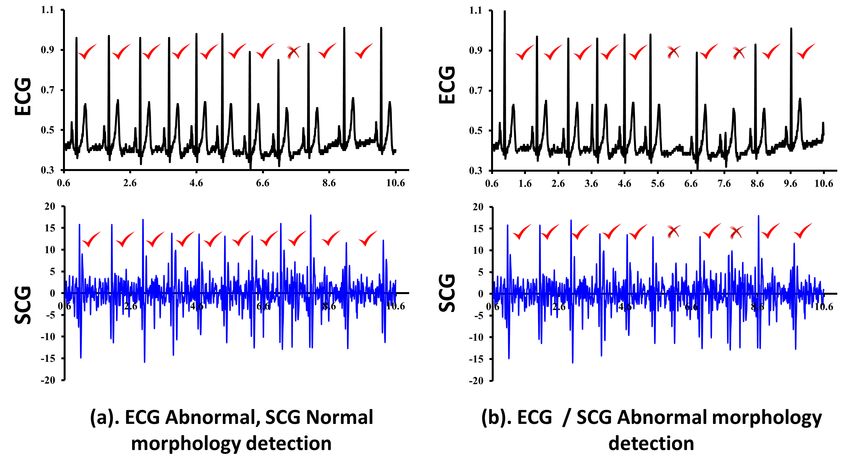
Sensors 2018, 18, 379 6 of 28
4. Cardiological Data Analysis
In this section, we introduce various feature points of ECG and SCG along with corresponding
values to distinguish between normal and abnormal cardiological data, followed by ECG/SCG based
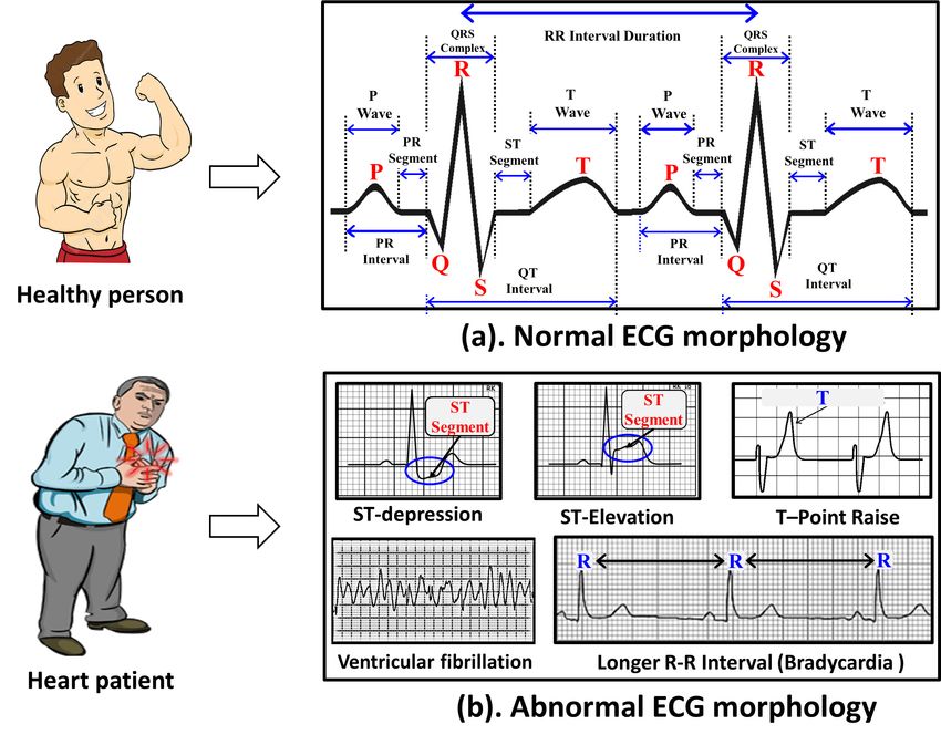
feature points delineations and cardiac health monitoring methods. The ECG and SCG cardiac
signals with corresponding cardiac electrical and mechanical activities are explained as shown in
Figure 2 using the normal ECG waveform aligned with the normal SCG waveform. The ventricle
depolarization, a cardiac electrical activity that takes place during the QRS complex can be represented
by the corresponding cardiac mechanical activities that take place between atrial systole AS to the
opening of aortic valve AO. Similarly, during the ventricle re-polarization (T wave) of ECG, the cardiac
mechanical activity such as rapid ejection of blood flow RE takes place until the closing of aortic valve
AC. Finally, during the atrial depolarization represented as P wave, cardiac mechanical activity known
as rapid diastolic filling RF can be observed.
Figure 2. Cardiac electrical and mechanical activities.
4.1. Differentiation between Normal and Abnormal ECG Morphology
For a normal and healthy heart, each heartbeat reflects an orderly progression of depolarization
in ECG tracing, which is helpful to know various heart functionalities. As shown in Figure 3a,
the normal ECG cycle is comprised of several cardiac electrical activities known as depolarization
and re-polarization responsible for heart muscular activities. The entire process of depolarization and
re-polarization of a cardiac cycle can be explained as follows. The ECG P wave represents the atrial
depolarization spreads from sinoatrial (SA) node throughout the atria followed by brief period of zero
voltage isoelectric representing delay at atrioventricular (AV) node. The QRS complex represents the
short duration of ventricular depolarization followed by ventricular re-polarization represented by T
wave. The ST segment between QRS complex and T wave represents the brief period of zero voltage
isoelectric, when both ventricles are completely depolarized. To define the normal and abnormal
behavior of depolarization, ECG trace is first divided into a set of heartbeat cycles. Each heartbeat
cycle is again sub-divided into various waves, segments, and interval such as P wave, QRS wave,
T wave, PR segment, ST segment, PR interval, and QT interval. The subdivision of heart beat cycle
into waves, segments, and intervals is performed based on the position and order of the ECG cardiac
feature points P, Q, R, S and T as shown in Figure 3a. In addition, RR interval duration can also be
used as a measure to decide between the normal and abnormal behavior of two consecutive heartbeats.
Table 1 shows the notations used in this paper to represent reference maximum and a minimum
value of waves, segments, and intervals observed in a normal ECG tracing. Cardiac anomalies such as
myocardial infarction, ischemia, sinus arrhythmia, sinus bradycardia, atrial/ventricular fibrillation,
etc., disturb the orderly progression of depolarization, and hence morphology of various waves,
segments and intervals changes significantly. Figure 3b shows various prominent ECG anomalies.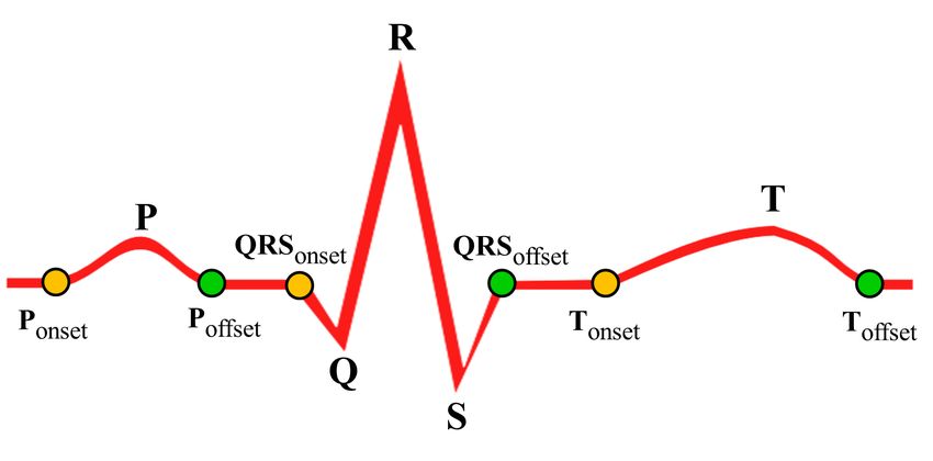
Sensors 2018, 18, 379                                                                            7 of 28

For example, in ST depression, a line at ST segment significantly bends downward below the isoelectric
line due to stable/unstable angina problem of a patient. On the other hand, in ST elevation, a line at
ST segment bends significantly upward above the isoelectric line due to non-transmural ischemia.
Moreover, bradycardia, characterized by a longer RR interval, can cause symptoms such as dizziness,
fatigue, chest pain etc. Although ECG is widely used to identify various cardiac anomalies, it may lead
to the wrong diagnosis and may falsely indicate the presence of CVD in patients with minor symptoms
of negligible risk to CVD [7]. Hence, it is necessary to correlate the abnormal behaviors observed in
ECG trace with the corresponding SCG trace to ensure the reliable cardiac health monitoring. The
following section describes the process of feature points delineation for ECG and SCG traces.

                          Figure 3. Example of normal and abnormal ECG morphologies.

                        Table 1. Notations for set of referenced normal feature values (RFV).

                               Notation                        Meaning
                                ∆Xwv         Referenced maximum X wave duration
                                δXwv          Referenced minimum X wave duration
                                ∆Yinv       Referenced maximum Y interval duration
                                δYinv       Referenced minimum Y interval duration
                                ∆Zseg       Referenced maximum Z segment duration
                                δZseg       Referenced minimum Z segment duration
                                ΩXwv        Referenced maximum X wave amplitude
                                ωPwv         Referenced minimum X wave amplitude
                                Here, X ∈ { P, QRS, T }, Y ∈ { RR, PR, QT }, Z ∈ { PR, ST }.

4.2. Feature Points Delineation Mechanism
     In this subsection, we present two separate mechanisms, one for ECG and another for SCG,
to select the corresponding feature points. Five ECG feature points such as P, Q, R, S, and T, and
nine SCG feature points such as AS, MC, I M, AO, IC, RE, AC, MO, and RF are considered. Figure 4
shows an example normal/abnormal ECG trace along with five ECG feature points selected by using
the proposed ECG feature points delineation algorithm. Similarly, Figure 5 shows an example SCG
trace with nine SCG feature points selected by the proposed SCG feature point delineation mechanism.
However, it is expected that the proposed ECG/SCG feature point delineation mechanisms should
select the corresponding feature points from normal as well as abnormal ECG/SCG traces, it is to note
that cardiac anomalies such as ventricular fibrillation shown in Figure 3b may result in non-detection
Sensors 2018, 18, 379 8 of 28
of few or all feature points. Here, it is assumed that ECG and SCG traces are collected in the form of
vectors of data points represented as Vecg and Vscg with known sampling rate Sr and mean heart rate Hr .
Each sampled ECG and SCG data point in Vecg and Vscg represents unique amplitude value in terms of
millivolts (mV). All of the local maximum and minimum peaks in ECG/SCG cycles are identified using
second derivatives with slope value zero to measure the corresponding ECG/SCG amplitude. The
measured amplitude represents the sensor value minus the baseline, where the baseline amplitude is
computed as zero voltage of ECG/SCG signal. For feature points’ delineation, both methodologies first
select the feature points in the first cardiac cycle and continue to select the feature points in subsequent
cardiac cycles with a minimum separation distance equivalent to the cardiac cycle length CL between
the same feature points. The sampling rate Sr and mean heart rate Hr are the known input parameters
1
of the experimental data sets used to estimate the cardiac cycle length represented as CL = ∗ Sr .
Hr
In practice, Hr is estimated continuously from the RR interval duration and updated to continuously
estimate the CL.
Figure 4. Feature points delineation in (a) normal ECG cycles; (b) abnormal ECG cycles.
Figure 5. Feature points delineation in (a) normal SCG cycles; (b) abnormal SCG cycles.Sensors 2018, 18, 379 9 of 28
4.2.1. ECG Feature Points Delineation Mechanism
For ECG trace, at first, the feature point R is selected and then after rest feature points Q, R,
S and T are selected with respect to R considering the referenced normal values of various waves,
intervals, and segments as reported in [32,33]. Although normal referenced values may not be the
best indicators to detect the very specific heart diseases, they can act as sufficient estimators under
quite a bit distorted morphologies for the unobtrusive cardiac health monitoring. Normally, feature
point R exhibits high amplitude, which is easy to detect. The process of feature point R detection can
be described as follows. Firstly, a unique peak ζ pt exhibiting the maximum amplitude is identified
from all the cardiac cycles under consideration. Later, all the peaks in a cardiac cycle with amplitude
greater than σR pt × ζ pt are chosen as candidate R peaks represented as cnR pts . Here, σR pt is a constant
between 0 and 1, which must be determined experimentally. In the current study, the σR pt = 0.7 is
obtained experimentally, which provides consistently superior performance as shown in Figure 6a.
Finally, the peak exhibiting maximum amplitude among cnR pts in a cardiac cycle is designated as
feature point R and is represented by R pt .
Figure 6. Evaluation of delineation of ECG feature point R and SCG feature point AO.
The feature points’ delineation other than R is a non-trivial process, and therefore feature point
specific range is formulated in such a way that it maximizes the chances of respective feature point
delineation. Four ranges of data points represented as Qrg , Prg , Srg , and Trg are formulated with respect
to the feature point R to select ECG feature points Q, P, S and T, respectively. The range format for
feature points appearing before and after R is formulated as ( R pt − Y, R pt ) and ( R pt , R pt + (Y + α)),
respectively. Here, Y represents the set of data points equivalent to the normal wave duration of the
∆QRSwv ∗ Sr
corresponding feature point. For example, for feature point Q, Y = . However, to reduce
2
the estimation error of Y, an error margin constant α is added as a precautionary measure to get
better estimation of feature-point range Y. Here, ∆QRSwv represents the normal time duration of
the QRS wave, and Sr represents the sampling frequency. For each feature point, the corresponding
peak is identified and designated as a feature point based on the minima and maxima characteristic.
For example, the peak representing the feature point Q in ECG normally appears as minima and
therefore the minimum peak from the range is designated as Q pt . A similar process is repeated for
each feature point except R in each ECG cardiac cycle. The entire process in the form of pseudo-code is
given in Algorithm 1.
Besides delineation of ECG feature points, it is also essential to delineate end points of the
waves. The ECG end points of waves can be classified into two sets. The set of onset pointsSensors 2018, 18, 379 10 of 28
such as { Ponset , QRSonset , Tonset }, and the set of offset points { Po f f set , QRSo f f set , To f f set } as shown
in Figure 7. In many instances, due to the cardiac abnormalities such as left/right atrial enlargement,
ST elevation/depression, and T point raise, the delineation of end points become difficult. In particular,
the delineation of end points in case of flatten/inverted T waves is painful. Hence, a simple end
point delineation mechanism is incorporated. At first, using the duration of P wave, QRS complex
rg rg rg
and T wave observed in normal ECG cycles, the set of onset range { Ponset , QRSonset , Tonset } and
rg rg rg
the set of offset range { Po f f set , QRSo f f set , To f f set } are derived with respect to the feature points P,
R and T, respectively. Finally, the data point with minimum amplitude value is located within the
rg rg rg rg
range Ponset , Tonset , Po f f set and To f f set and annotated with Ponset , Tonset , Po f f set and To f f set , respectively.
rg
Similarly, QRSonset and QRSo f f set are located as the maximum data points within the range QRSonset
rg
and QRSo f f set , respectively.
4.2.2. SCG Feature Points Delineation Mechanism
Similar approach of ECG is adopted while selecting various feature points from the SCG trace,
where, at first, feature point AO is selected and then rest eight feature points AS, MC, I M, IC, RE, AC,
MO, and RF are selected with respect to the position of AO. One of the distinguished properties of SCG
is the unusual high amplitude of feature point AO in SCG morphology as shown in Figure 5, which
makes it easy for the delineation of AO in a cardiac cycle. However, this does not hold true in every
cardiac cycles and is valid under the specific constraints. For example, in a clear SCG morphology of a
healthy subject, AO normally exhibits high amplitude in most cycles with few exceptions. However,
in distorted SCG morphology of an unhealthy subject, the delineation of AO is more complicated and
may give poor results. Similar to selecting R in ECG feature point delineation, maximum amplitude
peak ζ pt from the set of cardiac cycles is located first. Then, for each individual cardiac cycle, the set
of candidate AO peaks represented as cnAO pts are located with amplitude more than σAO pt × ζ pt .
Here, σAO pt is a user-defined constant between 0 and 1, which can be obtained experimentally. In the
current study, σAO pt = 0.75 is found to give consistently superior performance as shown in Figure 6b.
Finally, from the set cnAO pts , a unique peak exhibiting maximum amplitude is designated as SCG
feature point AO represented by AO pt .
SCG morphology is more complex in nature as compared to ECG and therefore it requires
significant efforts to correctly locate the feature points other than AO. Since SCG morphology is not
well studied, the normal representative value of an amplitude of various peaks and duration of waves
are not yet well defined in the literature. Hence, set of training SCG cardiac cycles from the healthy
subjects are used to estimate the distance (i.e., the window size) of various SCG feature points with
respect to AO to formulate feature point specific range. The window size calculated from the training
SCG cycles of healthy population has dual advantages: (1) it helps to estimate the normal window size
for healthy subjects; and (2) it also helps to identify the significantly varying abnormal SCG features
lying outside the normal window size (e.g., outliers), which is observed among non-healthy subjects.
For each SCG feature point, a fixed size range Xrg consisting of probable data points is formulated at the
obtained feature point specific window size SW ( X ), where X ∈ { AS, MC, I M, IC, RE, AC, MO, RF }.
Finally, based on the morphological maxima or minima characteristic of each feature point, a unique
peak is obtained from the Xrg and is designated as a feature point. For example, for SCG feature
point AS, range ASrg of probable data points for AS at distance SW ( AS) is formulated with respect to
AO. Subsequently, the peak with maximum amplitude in the range of ASrg + α is designated as SCG
feature point AS pt . A similar approach is followed for the delineation of all other SCG feature points.
Detailed pseudo code for SCG feature points’ delineation is described in Algorithm 2.Sensors 2018, 18, 379 11 of 28
Algorithm 1: Delineation of ECG feature points.
Input:
Vecg : Vector of ECG data points with amplitude, Sr : ECG data sampling rate,
Hr : Heart rate, RFV : Set of referenced feature values.
Output:
Fecg = { P, Q, R, S, T } : ECG feature point set.
Notations:
ζ pt : Maximum amplitude data point,
cnR pts : Candidate R points,
Xrg : Range of points to locate point X, where X ∈ { P, Q, S, T },
α: User defined error margin constant,
σR pt ∈ (0, 1): Constant to detect R points,
a : ECG feature point set for ath cardiac cycle.
Fecg
1 Initialize Fecg = null;
Sr
2 Estimate cardiac cycle length: CL = Hr ;
|Vecg |
3 Calculate # of cardiac cycles: CCs = CL ;
1 , ..., V |Vecg |
4 Select maximum amplitude data point: ζ pt = max (Vecg ecg );
5 for a = 1 to CCs do
6
a = null;
Initialize Fecg
j
7 Select candidate R points: cnR pts = (Vecg ≥ σR pt ∗ ζ pt ), ∀ j ∈ Vecg ;
8 R pt = max (cnR pts ); // Delineation of feature point R.;
9
a = Fa ∪ R ;
Fecg pt
ecg
∆QRSwv ∗ Sr
10 Qrg = R pt − ( + α), R pt ;
2
j
11 Q pt = min(Vecg ), ∀ j ∈ Qrg ; // Delineation of feature point Q.;
12
a = Fa ∪ Q ;
Fecg pt
ecg
13 Prg = R pt − (∆PRinv ∗ Sr + α), R pt ;
j
14 Ppt = max (Vecg ), ∀ j ∈ Prg ; // Delineation of feature point P.;
15
a = Fa ∪ P ;
Fecg pt
ecg
∆QRSwv ∗ Sr
16 Srg = R pt , R pt + ( + α) ;
2
j
17 S pt = min(Vecg ), ∀ j ∈ Srg ; // Delineation of feature point S.;
18
a = F a ∪ QRS ;
Fecg pt
ecg
∆QRSwv ∗ Sr
19 Trg = R pt , R pt + (∆QTinv ∗ Sr − + α) ;
2
j
20 Tpt = max (Vecg ), ∀ j ∈ Trg ; // Delineation of feature point T.;
21
a = Fa ∪ T ;
Fecg ecg pt
22
a ;
Fecg = Fecg ∪ Fecg
23 endfor
24 return Fecg ;Sensors 2018, 18, 379 12 of 28
Figure 7. Example of ECG feature points, onset points and offset points.
4.3. Data Analysis Methodology
In this subsection, we present mechanisms to differentiate between normal and abnormal
morphology of ECG and SCG cardiac cycles.
4.3.1. Abnormal ECG Morphology Detection
The cardiac abnormal morphology in ECG trace either appear in the form of significant variation
in amplitude of feature points P, Q, R, S, and T, or appear in the form of significant variation in the
duration of waves i.e., P, QRS, T, segments i.e., ST, PR, and intervals i.e., RR, PR, ST, and QT. In this
paper, the abnormal morphology related to P wave, QRS complex, and T wave is determined with
respect to the referenced amplitude and wave durations as suggested in [32]. It is observed that critical
cardiac anomalies in a patient normally last a little longer and affect multiple consecutive heartbeats.
Therefore, cardiac abnormalities that arise in an individual heartbeat due to occasional uncommon
amplitude and duration are ignored. Instead of monitoring cardiac cycles individually, the group
of cardiac cycles is monitored together such as 5-cycles, 10-cycles, 25-cycles, and 50-cycles, etc. The
purpose of considering the group of cardiac cycles is to ensure that robust cardiac abnormalities are
captured by the system instead of the system being misguided by occasional false abnormalities that
arise due to bad signal quality and external noises.
The cardiac abnormal morphology count is maintained, which is increased each time by one,
whenever amplitude, wave duration, or both vary substantially with respect to their corresponding
reference values. Finally, at the completion of the group of cardiac cycles, a feature point with
a maximum number of cardiac abnormalities is considered as the abnormal feature point. The
pseudo-code for abnormal morphology detection in ECG trace for the group of k-cycles is shown in
Algorithm 3, where k is a user-defined constant. Here, it is assumed that ECG signals are available in
i , where i = {1, 2, ..., |V |} represents set of data points sampled with sampling
the form of vector Vecg ecg
rate Sr .Sensors 2018, 18, 379 13 of 28
Algorithm 2: Delineation of SCG feature points.
Input:
Vscg : Vector of SCG data points with amplitude, Sr : SCG data sampling rate, Hr : Heart rate.
Output:
Fscg = { AS, MC, I M, AO, IC, RE, AC, MO, RF } : SCG feature point set.;
Notations:
ζ pt : Maximum amplitude data point, cnAO pts : Candidate AO points, Xrg : Range of points to
locate point X, where X ∈ { AS, MC, I M, IC, RE, AC, MO, RF },
SW ( X ) = Range of probable data points in sliding window of SCG feature point X,
Φ: Set of manually annotated normal training SCG cycles, α: User defined error margin
a : SCG feature point set for
constant, σAO pt ∈ (0, 1): Constant to detect AO points, Fscg
th
a cardiac cycle.
1 Initialize Φ as training data set ;
2 Estimate SW ( X ) with respect to AO for each training cycle in Φ ;
3 Initialize Fscg = null;
S
4 Estimate cardiac cycle length: CL = Hr ;
r
|Vscg |
5 Calculate # of cardiac cycles: CCs = CL ;
1 , ..., V |Vscg |
6 Select maximum amplitude data point: ζ pt = max (Vscg scg );
7 for a = 1 to CCs do
8
a = null;
Initialize Fscg
j
9 Select candidate AO points: cnAO pts = (Vscg ≥ σAO pt ∗ ζ pt ), ∀ j ∈ Vscg ;
10 AO pt = max (cnAO pts ); // Delineation of feature point AO.;
11
a = F a ∪ AO ;
Fscg scg pt
12 endfor
13 Load SCG testing dataset Vscg ;
14 for a = 1 to CCs do
15 foreach AO − AO duration do
16
a = null;
Initialize Fscg
17 ASrg = SW ( AS) ± α ;
j
18 AS pt = max (Vscg ), ∀ j ∈ ASrg // Delineation of feature point AS.;
19 MCrg = SW ( MC ) ± α ;
j
20 MC pt = max (Vscg ), ∀ j ∈ MCrg // Delineation of feature point MC.;
21 I Mrg = SW ( I M ) ± α ;
j
22 I M pt = min(Vscg ), ∀ j ∈ I Mrg // Delineation of feature point I M.;
23 ICrg = SW ( IC ) ± α ;
j
24 IC pt = min(Vscg ), ∀ j ∈ ICrg // Delineation of feature point IC.;
25 RErg = SW ( RE) ± α ;
j
26 RE pt = max (Vscg ), ∀ j ∈ RErg // Delineation of feature point RE.;
27 ACrg = SW ( AC ) ± α ;
j
28 AC pt = max (Vscg ), ∀ j ∈ ACrg // Delineation of feature point AC.;
29 MOrg = SW ( MO) ± α ;
j
30 MO pt = min(Vscg ), ∀ j ∈ MOrg // Delineation of feature point MO.;
31 RFrg = SW ( RF ) ± α ;
j
32 RFpt = max (Vscg ), ∀ j ∈ RFrg // Delineation of feature point RF.;
33
a = F a ∪ AS ∪ MC ∪ I M ∪ IC ∪ RE ∪ AC ∪ MO ∪ RF ;
Fscg scg pt pt pt pt pt pt pt pt
34 end
35
a ;
Fscg = Fscg ∪ Fscg
36 endfor
37 return Fscg ;Sensors 2018, 18, 379 14 of 28
Algorithm 3: Abnormal ECG morphology detection
Input:
Vecg : Vector of ECG data points with amplitude, Sr : ECG data sampling rate,
Hr : Heart rate, RFV : Set of referenced feature values, k : User defined constant to group
k-cycles.
Output: Detection of abnormal morphologies
Notations:
θXwv : Measured amplitude of X wave,
ψXwv : Measured duration of X wave,
cXwv : Counter for X wave abnormal morphologies, where X ∈ { P, QRS, T },
cRRinv : Counter for RR interval abnormal morphologies,
ψRRinv : Measured duration of RR interval.
1 Initialize k;
2 Initialize cPwv = cQRSwv = cTwv = cRRinv = 0;
S
3 Estimate Cardiac cycle Length: CL = Hr ;
r
|V |
ecg
4 Calculate # of cardiac cycles: CCs = CL ;
5 for i = 1 to CCs − k + 1 do
6 j=i;
7 while j ≤ (i + k) do
8 if (θPwv > ΩPwv ) ∨ (θPwv < ωPwv ) ∨ (ψPwv > ∆Pwv ) ∨ (ψPwv < δPwv ) then
9 cPwv = cPwv + 1; // P wave abnormal morphology detection
10 end
11 ;
12 if (θQRSwv > ΩQRSwv ) ∨ (θQRSwv < ωQRSwv ) ∨ (ψQRSwv >
∆QRSwv ) ∨ (ψQRSwv < δPwv ) then
13 cQRSwv = cQRSwv + 1; // QRS wave abnormal morphology detection;
14 end
15 if (θTwv > ΩTwv ) ∨ (θTwv < ωTwv ) ∨ (ψTwv > ∆Twv ) ∨ (ψTwv < δTwv ) then
16 cTwv = cTwv + 1; // T wave abnormal morphology detection;
17 end
18 if (ψRRinv > ∆RRinv ) ∨ (ψRRinv < δRRinv ) then
19 cRRinv = cRRinv + 1; // RRinv interval abnormal morphology detection;
20 end
21 end
22 endfor
At first, from the past studies [32,33], a set of reference values RFV is formulated. The RFV
consists of reference normal values corresponding to an amplitude of feature points and duration
of waves, segments, and intervals. The set RFV represents the reference normal values within two
standard deviations from the mean with percentile range of 2% through 98% of healthy subjects.
Table 1 defines the notations that are used to represent the reference values used in Algorithm 3.
i , S , H , and a set RFV are considered as input to Algorithm 3 to detect the cardiac abnormal
Vecg r r
cycles in ECG trace. In each cardiac cycle, the current measured value of amplitude, wave, segment,
and interval duration of each feature point is compared with the corresponding reference normal
values. As shown in Algorithm 3, in cardiac abnormality detection of P, the current measured value of
amplitude θPwv and wave duration ψPwv are compared with the reference minimum and maximum
value of amplitude (i.e., ΩPwv and ωPwv ) and wave duration (i.e., ∆Pwv and δPwv ), respectively. The P
wave cardiac abnormal morphology counter cPwv is maintained, which is increased by one in eachSensors 2018, 18, 379 15 of 28
time, either measured amplitude θPwv or wave duration ψPwv lies outside the reference normal values.
The similar approach is followed to detect the abnormal morphology of QRSwv , Twv and RRinv .
4.3.2. Abnormal SCG Morphology Detection
As far as our knowledge is concerned, there exists no well-studied method to detect the abnormal
morphology of SCG cardiac cycles. The existing literature mainly focuses on the delineation of
SCG feature points [6,8,23] or focuses on the applicability of SCG in the diagnosis of cardiac health
problems [20,23–25]. In this subsection, a process to identify abnormal morphologies in an SCG cardiac
cycle is described. Since SCG is employed as an additional measure to complement the performance
of ECG based monitoring, the SCG feature points’ delineation and designing of feature-variables
are made independent from the ECG to avoid any sorts of performance influence on SCG. Six SCG
feature variables are designed to detect morphological abnormalities in SCG cardiac cycles such as
Π MC,AO , Π AO,AC , Π MC,MO , Π AC,MO , Π RBE , and Π RBF . These six SCG feature-variables represent the
duration of various cardiac mechanical activities that take place in a cardiac cycle. The notation of
SCG feature-variables along with their corresponding cardiac mechanical activities are described in
Table 2. Due to the sensitive nature of SCG accelerometer sensors, the amplitude behavior of various
SCG feature points is observed highly fluctuating. Therefore, the only parameter considered important
to design SCG feature-variables is the duration of cardiac mechanical activities ignoring the amplitude
parameter. In this paper, an SCG cardiac mechanical activity is considered abnormal, whenever
significant variation is observed in the duration of corresponding SCG feature-variable with respect to
the normal duration. Figure 8 shows the derivation of SCG feature-variables from the SCG signal.
Table 2. Notation of SCG feature-variables.
Notation Meaning
Π MC,AO Time Duration from closing of mitral to opening of aortic.
Π AO,AC Time duration between opening and closing of aortic.
Π MC,MO Time duration between closing and opening of mitral.
Π AC,MO Time duration from closing of aortic to opening of mitral.
Π RBE Time duration of ventricle blood ejection.
Π RBF Time duration of diastolic blood filling.
FVscg = {Π MC,AO , Π AO,AC , Π MC,MO , Π AC,MO , Π RBE , Π RBF }.
Figure 8. Feature-variables derived from SCG Tricuspid valve site.
In contrast to ECG, SCG does not have predefined referenced values to detect the abnormal
behavior of feature-variables. Therefore, the reference value of each SCG feature-variable is first
estimated from η number of initial SCG cardiac cycles from a set of five subjects. It is to be notedSensors 2018, 18, 379 16 of 28
that the estimation of SCG reference values is the mean representation of five subjects. For a given
subject and heart rate, these reference time intervals are first normalized and then the customized
subject-specific set of reference time intervals is obtained. Later, the estimated value of feature-variables
is used to measure the significant variation of feature-variables for a given subject. Here, η can be
defined experimentally and it varies from one data set to another. The smaller the value of η, the more
premature the estimation is observed and the higher the value of η, the more error propagation is
observed. Hence, a trade-off needs to be balanced for optimum estimation of η. In this paper, the value
of η is kept to 20 cardiac cycles, which consistently performs better to estimate the feature-variables
with reasonable accuracy. The first η number of cardiac cycles is considered as an estimation phase,
during which a cardiac abnormality detection process is not initiated; rather, duration of various
feature-variables is estimated.
In the estimation phase, time series analysis of data is performed to smoothen out short-term
fluctuations and to capture the long-term trend of feature-variables. Moreover, behavioral changes
such as respirations and body movements are also accommodated in time-series signal analysis by
assigning weights to the cardiac cycles in the decreasing order. The weighted moving average duration
WavgDi and weighted moving standard deviation duration WstdDi are calculated for each individual
feature-variable-i, where i ∈ FVscg . At the end of the η number of cardiac cycles, the value of WavgDi
and WstdDi are used as the decision values to detect the cardiac abnormalities in the duration of
feature-variables in subsequent cardiac cycles.
In estimation phase, WavgDik is calculated using Equation (1) and WstdDik is calculated using
Equations (2) and (3) for η number of cardiac cycles, where i represents the ith feature-variable and k
represents the kth cardiac cycle. Here, Dik represents the measured time duration of ith feature-variable
in kth cardiac cycle, where i ∈ FVscg :
Dik , i f k < η,
η
∑k=1 k × Dik
WavgDik = η , i f k = η, (1)
∑ k =1 k
k −1 η k k −1
WavgDi + ∑η j ( Di − WavgDi ), i f k > η.
j =1
To calculate WstdDik , continuous variance Sik is first calculated using Equation (2). The method to
calculate Sik is inspired from B. P. Welford’s method [34], which is an accurate and guaranteed way to
generate the non-negative variance under floating point calculations:
0, i f k = 1,
1
η k 2 k
k
Si = η ∑k=1 k × ( Di ) − WavgDi , i f k = η, (2)
∑ k =1 k
k −1
+ k × ( Dik − WavgDik−1 ) ∗ ( Dik − WavgDik ),
Si i f k > η.
From variance Sik , weighted moving standard deviation duration WstdDik is calculated as shown
in Equation (3):
s
Sik
WstdDik = f or k > η. (3)
( k − 1)Sensors 2018, 18, 379 17 of 28
Once the estimation phase is concluded and decision values WavgDik and WstdDik are obtained,
evaluation phase is initiated. During each cycle in the evaluation phase, the value of each feature-variable
Dik , where i ∈ FVscg and k > η is inspected against the range (WavgDik + WstdDik , WavgDik − WstdDik )
of corresponding feature-variable. If value of any feature-variable Dik is found lying outside the range
(WavgDik + WstdDik , WavgDik − WstdDik ), then the corresponding feature-variable is considered as
potential outlier and it is marked as abnormal. Since the distribution of value of feature-variables
with respect to the mean of corresponding feature-variable can be considered as Gaussian distribution,
we used Chauvenet’s criterion [35] to identify outliers in each cycle of the evaluation phase. In order
to identify the outliers, deviation devDi and tolerance tolDi for each feature variable-i is calculated
using Equations (4) and (5), respectively:
Dik − WavgDik−1
devDi = f or η ≤ k ≤ CCs, (4)
WstdDik−1
1
tolDi = NORM.S.I NV ( ). f or η ≤ k ≤ CCs. (5)
4∗k
Here, NORM.S.I NV indicates the inverse of standard normal cumulative distribution and CCs
represents the total number of cardiac cycles. According to the empirical rule of statistics, in Gaussian
distribution, 95% of data lies within two standard deviations from the mean and hence as per the
thumb rule, one should consider no more than 5% of data as outliers. Hence, the value of tolerance
tolDi is calculated in such a way that for those feature-variables whose duration value deviates more
than two standard deviations from the mean of the corresponding feature variable is considered
as outliers.
4.4. Combined Analysis of ECG and SCG Signals
Once the detection of the various types of abnormal morphologies is concluded from ECG
and SCG signals. The next step is to ascertain that the cardiac cycle under consideration is indeed
abnormal. Since, mere the detection of abnormal morphologies does not mean the abnormal behavior
of the cardiac cycle, a Naïve Bayes probabilistic model is designed to know how likely the cardiac
cycle under consideration is to be abnormal. For the probabilistic model design, ECG feature set
consisting of seven features is used, which is represented as FVecg = {ΘXwv , ψXwv , ψRRinv }. Here,
X ∈ { P, QRS, T }, and Θ and ψ represents measured wave amplitude, and duration, respectively.
Similarly, SCG feature set consisting of six features is used, which is represented as FVscg =
{Π MC,AO , Π AO,AC , Π MC,MO , Π AC,MO , Π RBE , Π RBF }.
The conditional Naïve Bayes probability model is designed to classify each cardiac cycle into
class normal or abnormal. Let us say that for the kth ECG cardiac cycle with feature set FVecg k =
{ΘXwvk , ψX k , ψRRk }, the conditional probability for a cardiac cycle to be normal or abnormal can be
wv inv
defined as shown in Equation (6):
k |ϕ )
p( ϕl ) × p( FVecg
k l
p( ϕl | FVecg )= k )
, where l ∈ {1, 2}. (6)
p( FVecg
k )
Here, ϕl =1 and ϕl =2 represents output class normal and abnormal, respectively. The p( ϕl =1 | FVecg
k th
and p( ϕl =2 | FVecg ) represents the probability of k cardiac cycle to be normal and abnormal,Sensors 2018, 18, 379 18 of 28
k . The p ( ϕ | FV k ) can be rewritten as shown in
respectively, for a given ECG feature set FVecg l ecg
Equation (7):
k k k k
p( ϕl | FVecg ) = p( ϕl |ΘXwv , ψXwv , ψRRinv ). (7)
k is assumed
Under the Naïve Bayes conditional independence assumption, each feature xi ∈ FVecg
k for j 6 = i. Hence, Equation (7) can be
conditionally independent to every other features x j ∈ FVecg
simplified as follows:
k k k k k k
p( ϕl |ΘXwv , ψXwv , ψRRinv ) ∝ p( ϕl , ΘXwv , ψXwv , ψRRinv )
k k k
∝ p( ϕl ) × p(ΘXwv | ϕl ) × p(ψXwv | ϕl ) × p(ψRRinv | ϕl )
i =6
∝ p( ϕl ) × ∏ p( xi | ϕl ), where xi ∈ FVecg
k
i =1
i =6
= Ξ × p( ϕl ) × ∏ p( xi | ϕl ), Here, Ξ is a constant. (8)
i =1
The Naïve Bayes conditional probability model defined in Equation (8) can be transformed into
classifier using the maximum a posteriori decision rule as follows:
i =6
Γecg = arg max p( ϕl ) × ∏ p( xi | ϕl ), where xi ∈ FVecg
k
. (9)
l ∈{1,2} i =1
Similarly, the Naïve Bayes conditional probability classifier as shown in Equation (10) can be
constructed for SCG using a set of seven SCG features:
i =7
Γscg = arg max p( ϕl ) × ∏ p(yi | ϕl ), where yi ∈ FVscg
k
. (10)
l ∈{1,2} i =1
Here, Γecg and Γscg is assigned with class label ϕl for some l based on the maximum a posteriori
probability. Using the probabilistic outcome of Γecg and Γscg , each ECG and SCG cardiac cycle is
marked as normal (i.e., binary ’0’) or abnormal (i.e., binary ’1’):
k k
Joutcome = CCecg ∧ CCscg , (11)
# o f abnormal CCs in a group
CAI = . (12)
Total # o f CCs in a group
As mentioned in earlier sections, abnormalities in ECG cycles do not necessarily indicate the
underlying abnormal cardiac activities and therefore we look for the abnormalities in corresponding
SCG cardiac cycles as well. For an ECG and corresponding SCG cardiac cycle, if only one of them is
detected abnormal (e.g., binary ’1’) by proposed Naïve Bayes probabilistic classifier, then a conclusion
is drawn that the cardiac cycle under consideration is more likely to be normal in nature (e.g., binary
’0’) and observed abnormal morphology in either ECG or SCG cardiac cycle is due to the external
reasons such as noise. However, if both ECG as well as corresponding SCG cardiac cycles are
simultaneously detected with abnormal morphology, then a conclusion is drawn that the cardiac
cycle under consideration is indeed abnormal. Equation (11) acts as an additional measure to generate
reliable outcomes in the presence of signal artifacts. For example, if one of the modalities (let us say
ECG) outputs the abnormal cardiac cycle (e.g., binary 1) due to external signal artifacts, and the other
one (let us say SCG) outputs as entirely normal (e.g., binary 0), then the concerned cardiac cycle is
treated as normal ( e.g., 1 ∧ 0 = 0) to reduce the false positives and to avoid the mis-interpretation ofSensors 2018, 18, 379 19 of 28
results. The outcome of the combined analysis of ECG and SCG cardiac cycle can be calculated as
shown in Equation (11). Here, CCecg k and CC k represent individual outcomes of k th cardiac cycle of
scg
ECG and SCG, respectively. The Joutcome represents the combined outcome. In addition, Table 3 shows
all possibilities that arise in Equation (11). A new parameter called Cardiac Abnormality Index (CAI)
is defined to represent the intensity of cardiac abnormal behavior. The CAI is defined as the number of
abnormal cardiac cycles out of the total number of cardiac cycles in a group as shown in Equation (12).
The higher the value of CAI, the higher the risk of CVD and vice versa. If CAI increases gradually
over the period of time and crosses the predefined threshold value δ, an alert warning may be issued
to the user to consult the cardiologist. It is to note that the value of δ can be determined in consultation
with the cardiologists.
Table 3. Combined analysis outcomes of ECG and SCG cardiac cycles.
k
CCecg k
CCscg Joutcome
0 0 0
0 1 0
1 0 0
1 1 1
Here, 0 = normal, 1 = abnormal.
5. Performance Evaluation
In this section, first, we describe the methodology that we have adopted to evaluate the
performance of proposed ECG and SCG feature point delineation mechanisms followed by
corresponding results. Since our proposed combined cardiac anomaly detection mechanism is based on
the investigation of various feature points of ECG and SCG signals, first we need to verify the accuracy
of the proposed ECG and SCG feature point delineation mechanisms. Performance evaluation is carried
out on 12,000 cardiac cycles of ECG and SCG collected from three normal (N) and two abnormal (AN)
real subjects using our IRB license as described in Section 2.
5.1. Demographic Information
For each subject, an individual data file comprised of ECG and SCG signals in the form of sampled
data points is generated as an output as part of data collection process. Total 20 subjects are recruited for
the data collection purpose with an equal number of male and female subjects, i.e., 10 subjects per gender.
The demographic information of the subjects is summarized in Table 4. The average age of the subjects
is 24.45 years and the age ranges from 21 through 30 years. The data collection for all the subjects is
carried out in supine posture as presented in Figure 1. Out of 20 subjects, 12 subjects are found as
normal and eight subjects are considered as abnormal due to their sedentary lifestyle. The average
height, weight, and BMI (Body Mass Index) of subjects is 1.52 (m), 59 (kg) and 22.9, respectively. In
addition, Table 4 shows an example of value of amplitude in mV out of thousands/millions of mV
measurements for the reference purpose only. The inclusion criteria are presumably healthy adult
subjects with no known cardiac conditions, equal number of male and female subjects with age ≥ 18;
whereas the exclusion criteria are the inability to provide written consents, sample size less than 20
subjects. For each subject, data collection is carried out for total 15 min consisting of three sessions of
5 min each with 5 min of a break between the successive sessions. It is to be noted that the entire data
collection process is thoroughly verified by approved by an ethical committee of Institution Review
Board (IRB) of Gung Memorial Hospital (CGMH), Taiwan with IRB license number 104-6615B.
All of the 20 subjects are chosen for experiment purposes. Since manual annotation is a highly
laborious process, we present results based on the case study of 20 subjects. However, without losing
the generality, it is to be noted that 12,000 cardiac cycles in total are considered from the selected
subjects for joint investigation, which are statistically sufficient enough to interpret the trend and toYou can also read