Human visual motion perception shows hallmarks of Bayesian structural inference - Nature
←
→
Page content transcription
If your browser does not render page correctly, please read the page content below
www.nature.com/scientificreports
OPEN Human visual motion perception
shows hallmarks of Bayesian
structural inference
Sichao Yang1,2,6*, Johannes Bill3,4,6*, Jan Drugowitsch3,5,7 & Samuel J. Gershman4,5,7
Motion relations in visual scenes carry an abundance of behaviorally relevant information, but little
is known about how humans identify the structure underlying a scene’s motion in the first place. We
studied the computations governing human motion structure identification in two psychophysics
experiments and found that perception of motion relations showed hallmarks of Bayesian structural
inference. At the heart of our research lies a tractable task design that enabled us to reveal the
signatures of probabilistic reasoning about latent structure. We found that a choice model based on
the task’s Bayesian ideal observer accurately matched many facets of human structural inference,
including task performance, perceptual error patterns, single-trial responses, participant-specific
differences, and subjective decision confidence—especially, when motion scenes were ambiguous and
when object motion was hierarchically nested within other moving reference frames. Our work can
guide future neuroscience experiments to reveal the neural mechanisms underlying higher-level visual
motion perception.
Motion relations in visual scenes are a rich source of information for our brains to make sense of our environ-
ment. We group coherently flying birds together to form a flock, predict the future trajectory of cars from the
traffic flow, and infer our own velocity from a high-dimensional stream of retinal input by decomposing self-
motion and object motion in the scene. We refer to these relations between velocities as motion structure.
In general, motion structure is not directly observable; it must be inferred from ambiguous sensory input.
Bayesian inference provides a principled mathematical framework for dealing with ambiguous input, and under-
standing visual motion perception within a Bayesian framework has a long history in perceptual psychology, with
applications to diverse phenomena: contrast-dependent speed perception1, perceptual biases originating from
partial occlusions of moving rigid o bjects2, the perception of superimposed drifting g ratings2,3, depth perception
of moving o bjects4, and speed perception of naturalistic s timuli5. This previous work, however, was focused on
elementary motion structures, in the sense that stimulus features either moved independently or were grouped
to form rigid objects. Our goal is to understand how more complex and realistic forms of structure are inferred.
To perform the challenging task of inferring realistic structures, our minds can leverage that many real-
world motion patterns are decomposable into hierarchical structures, that is, some motions are nested inside
others6. For example, the motion of flocking birds can be decomposed into shared and unique components.
Intuitively, we see the motion of a bird in terms of its motion relative to the reference frame of the flock, which
itself is perceived as a coherently moving object. Yet the concept of a flock motion is a latent variable that cannot
be observed directly. In fact, coherent motion is one of the principal cues that the visual system uses to group
visual features into o bjects7,8. Thus, the computational puzzle is to understand how hierarchical structure can
serve as both an organizing force, bringing order to the unruly circus of visual features, while also being inferred
from those same features.
Building on the seminal work of Gunnar J ohansson9, which first systematically studied hierarchical motion
decomposition in displays of moving dots, subsequent studies formalized the i dea10–12 and identified principles of
how motion components are extracted when multiple decompositions are possible13–15. Recently, Gershman et al.6
proposed a Bayesian framework for explaining motion structure discovery, using probabilistic inference over
hierarchical motion structures (they called motion trees). Subsequently, Bill et al.16 established experimentally
1
Department of Psychology, University of Wisconsin-Madison, Madison, USA. 2Max Planck Institute for
Biological Cybernetics, Tübingen, Germany. 3Department of Neurobiology, Harvard Medical School, Boston,
USA. 4Department of Psychology, Harvard University, Boston, USA. 5Center for Brain Science, Harvard University,
Boston, USA. 6These authors contributed equally: Sichao Yang and Johannes Bill. 7These authors jointly
supervised this work: Jan Drugowitsch and Samuel J. Gershman. *email: sichao@cs.wisc.edu; johannes_bill@
hms.harvard.edu
Scientific Reports | (2021) 11:3714 | https://doi.org/10.1038/s41598-021-82175-7 1
Vol.:(0123456789)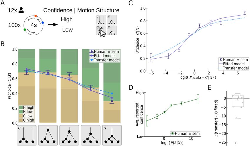
www.nature.com/scientificreports/
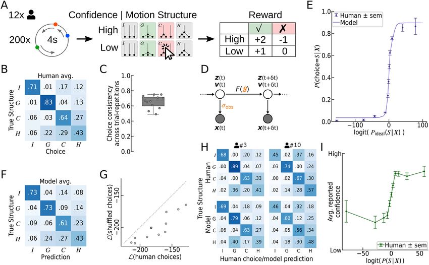
Figure 1. Motion structures used in Experiment 1. (A) Tree representations of 4 motion structures, each with
3 moving objects: independent (I), global (G), clustered (C), and hierarchical (H) motion. Next to each tree,
an example of the resulting motion patterns is provided. The motion structures are unobservable (latent), but
govern the velocity relations of the 3 visible objects (colored dots). In our formal representation of structure,
object velocities are driven by latent motion sources (non-leaf nodes in the graph; dashed boxes in the examples)
that affect the velocities of all connected downstream objects. Each motion source features a motion strength
(vertical edge length in the graph) with larger strengths corresponding to higher average velocities. For example,
the purple motion source drives the red and blue dots, either strongly (in structure C) or weakly (in H). (B) In
the experiments, colored dots moved along a circular track in order to make spatial relations among objects
uninformative. Dot colors were randomized in each trial. Here, a global (G) motion stimulus is illustrated.
that humans can exploit hierarchical structure when solving demanding visual tasks, such as object tracking
and trajectory prediction. However, in this study, participants were informed about the structure underlying
each trial, and the tested motion relations were designed to be clearly distinguishable. Thus, while this study
revealed which features of the structure were used by the visual system for solving a task, it remained unclear
whether participants could infer the underlying structure from sensory input in the first place. In particular,
Bill et al.16 did not address the computational principles which drive perception of latent motion structure and
explain occasional perceptual errors.
Here, we fill this gap by addressing the question how humans identify latent, hierarchical motion structure
in visual scenes. We do so by means of two theory-driven psychophysics experiments: alternative forced choice
tasks in which participants reported the perceived structure underlying short dynamic scenes. These experiments
go beyond previous work16 in that not only are object velocity percepts organized within a structure, but also
the structure itself is a latent variable that needs to be inferred. Furthermore, we designed the motion displays
such that stimuli could occasionally be ambiguous with regard to their underlying latent structure, thereby
probing perception in the face of uncertainty. Key to studying the specific contribution of motion structure to
perception is precise control over all object velocities. To this end, we employed a stimulus design that gener-
ates trials stochastically while endowing the experimenter with full control over the joint velocity distribution
of all visible objects. We were thereby able to eliminate several confounds that plague many traditional visual
motion displays, such as informative spatial arrangement of objects or informative low-level stimulus statistics.
As an additional benefit, the resulting visual scenes followed an analytically tractable generative model which,
when inverted according to Bayes’ rule, afforded an ideal observer of Bayesian structural inference. The ideal
observer enabled us to detect the behavioral signatures of structural inference that become apparent when the
evidence is ambiguous.
In our first experiment, we show that a choice model, which wraps a small set of known perceptual imper-
fections around an otherwise ideal Bayesian core, predicted many facets of human responses with high fidel-
ity. This included motion structure-specific task performance, distinct patterns of the confusability of certain
structures, predictions of responses with single-trial resolution, individual differences between participants, and
subjective confidence reporting. In our second experiment, we specifically targeted human perception of highly
ambiguous scenes, which we generated by morphing continuously between two prototypical motion structures.
The choice model again predicted human choice probabilities accurately. We conclude our study with a model
comparison revealing the differential contributions of the model’s components to explaining human motion
structural inference.
Results
Visual motion scenes with hierarchical structure. We adopted the hierarchical motion structure rep-
resentation from Gershman et al.6 and Bill et al.16, and the stimulus generation from Bill et al.16. Their main
components with respect to the present work are summarized in the following.
Graph representation of hierarchical structure. In Experiment 1, we focused on covert motion relations between
3 colored dots, using the 4 motion structures illustrated in Fig. 1A: independent (I), global (G), clustered (C), and
hierarchical (H) motion. In the case of independent motion, there are no correlations between the dots’ veloci-
ties. The independence is characterized in the graph structure (gray background in Figure 1A) by the absence of
shared ancestors between the 3 visible dots (colored nodes). The illustration next to the graph exemplifies the dot
velocities in a typical scene. For global (G) motion, a single latent motion source (gray node in the tree) is added,
which passes its velocity down to its descendants. In addition, each visible node features a smaller independent
motion component. Global motion describes, for example, to first order the velocities for a flock of birds. In
order to mathematically describe the coupling strength between the dots, we endow each source with a motion
strength (vertical extent of graph edges), with larger values of describing higher average velocities (see Mate-
rials and Methods for the mathematical definition). In the illustrated global motion scene, the shared motion
source is the dominant component to the dot velocities. The third motion structure is clustered (C) motion, in
Scientific Reports | (2021) 11:3714 | https://doi.org/10.1038/s41598-021-82175-7 2
Vol:.(1234567890)www.nature.com/scientificreports/
which 2 of the 3 dots share a latent motion source (purple node) while the 3rd dot moves independently. Finally,
in hierarchical (H) motion, two clustered dots and the 3rd dot are nested under an additional, global moving
reference frame. The fact that three is the smallest number of objects supporting such deeply-nested hierarchies
is why we chose a 3-dot stimulus design.
Stochastic generation of visual scenes. The graphs in Fig. 1A do not specify how a motion structure gives rise
to a concrete dynamic visual scene. We created motion scenes for our experiments using the stochastic stimu-
lus generation proposed in16 (see Materials and Methods for details). In this stimulus design, dot velocities
v(t) = (v1 (t), v2 (t), v3 (t)) follow a multivariate Ornstein–Uhlenbeck process17 in which latent motion sources
play the role of random forces which accelerate or decelerate the dots. The resulting velocity trajectories feature
the desired motion relations, obey our intuition that velocities change gradually due to inertia, and have an ana-
lytically tractable joint probability distribution. Analytical tractability enabled us to give all dots the same mar-
ginal speed distribution, independent of dot identities and the underlying motion structure. Thus, the velocity of
each dot taken alone was entirely uninformative about the motion structure. In addition, all dots were placed on
a circle, that is, v(t) describes their angular velocity (see Fig. 1B). Circular stochastic stimuli have the advantage
that they asymptotically break any spatial patterns between the dots, and thus leave correlations between veloci-
ties as the only information available for distinguishing different structures.
Humans can identify latent motion structure, but feature distinct error patterns. Using the
above-described stochastic motion scenes, we invited 12 participants to perform the visual motion structural
inference task illustrated in Fig. 2A. On each trial, a 4 s long dynamic scene with latent underlying motion
structure S ∈ {I, G, C, H} was presented on a computer screen (see Materials and Methods for details, and
Supplemental Video 1 for a screen recording of several trials). The structure S was drawn uniformly before
each trial, and remained fixed throughout the trial. After 4 s, the scene froze and the participant reported with
a mouse click the perceived structure and their level of confidence (low/high) in the decision. After the decision
was reported, the correct answer was revealed. Figure 2A exemplifies the feedback for a wrong choice (C), when
the correct answer was (G). For a low confidence decision, the participant received +1 point for correct answers
and 0 points for incorrect answers. For a high confidence decision, an additional point was “bet” which could
be matched (correct answer) or lost (wrong answer). Participants were aware of the 4 structures, received brief
training on the task, and conducted 200 trials (achieved score: 190 ± 33 points (mean ± SD)). In order to assess
the reliability of responses, the 200 trials of each participant consisted of only 100 unique scenes, each presented
twice in randomized order.
Our participants had a classification accuracy well above chance level for all four motion structures, as
evidenced by the confusion matrix shown in Fig. 2B. Yet, the different motion structures elicited distinct error
patterns. For example, participants tended to confuse clustered (C) and hierarchical (H) stimuli, or perceived
hierarchical motion as global (G). Interestingly, the confusability of motion structures often was not symmetrical,
as exemplified by the I-C and C-I elements of the confusion matrix. The spatial arrangement of the dots on the cir-
cle, in contrast, did not seem to have an influence on the perceived motion structure (see Supplemental Fig. S1),
in line with the uninformativeness of spatial arrangement in the task design. Furthermore, human responses
featured a truly stochastic component, as revealed by comparing their responses across the two unique-trial
repetitions (Fig. 2C). When re-presented with an identical scene, the same participant’s choice was consistent
with their previous choice only 65.2% ± 1.4% (s.e.m.) of the time. To summarize, our participants were generally
able to identify the structure underlying a motion scene. Yet, their responses featured stochasticity and systematic
error patterns, with some structures being more confusable than others.
Human motion perception is explained by a model of Bayesian structural inference. Errone-
ous identification of motion structures could arise either from false perceptual decision making or—owing to the
stochastic stimulus generation—from objective ambiguity of the presented scenes. To tease these factors apart,
we analyzed human responses from a normative standpoint of statistical inference. Concretely, we progressed
in two steps. First, we exploited the analytical tractability of the stimulus design to formulate a Bayesian ideal
observer. The ideal observer evaluates the likelihood p(X | S) of a presented trajectory, X := {x(t), 0 ≤ t ≤ T},
under the four alternative motion structures S and, thus, provides an objective statistical measure of a trial’s
most likely structure and of the statistical significance of this conjecture. In the second step, we devised a choice
model of human choices, P(choice = S | X), by augmenting the ideal observer with well-known imperfections of
human perceptual decision making (see Materials and Methods). The choice model featured a small number of
interpretable free parameters and afforded a deeper understanding of the computations driving human motion
structural inference. Both models and their implications are presented in the following.
The Bayesian ideal observer suggests statistically correct structural inference by humans. The analysis via an ideal
observer was made possible by the analytical tractability of the stimulus that obeyed the generative model shown
in Fig. 2D. True dot locations z(t) and velocities v(t) are latent variables that evolve according to a stochastic pro-
cess with correlated transitions F(S), which depend on the underlying latent structure S. For instance, a global
motion stimulus features positively correlated transitions of dot velocities. Ultimately, the correlated transitions
lead to temporal correlations among the observed locations x(t), which we assumed to be noisy observations
of z(t) at the times of the video frames, t = 0, δt, 2δt, . . . , T . The linear stochastic dynamics of the generative
process render Kalman filtering with a correlated state-transition model the ideal observer for these stimuli
(see Materials and Methods). In particular, Kalman filtering allows us to calculate the likelihood, p(X | S), of a
trial’s trajectory under any of the candidate motion structures, S = I, G, C, H . Thus, comparing the likelihoods
Scientific Reports | (2021) 11:3714 | https://doi.org/10.1038/s41598-021-82175-7 3
Vol.:(0123456789)www.nature.com/scientificreports/
Figure 2. Human perception of structured motion shows hallmarks of Bayesian structural inference.
(A) Illustration of Experiment 1. In each trial, a short scene of three moving dots was presented. The scene
was generated from a latent structure drawn randomly from the 4 structures in Fig. 1A. At the end of the trial,
participants reported the perceived structure (I/G/C/H) and their confidence (low/high) in that decision.
The correct structure was then revealed, and points were awarded based on correctness and confidence.
(B) Confusion matrix of human responses, averaged over all participants and trials. The (S, S′ ) element is the
empirical probability of choosing S′ in trials of structure S. Humans perform clearly above chance (0.25), but
show a reliable pattern of errors. (C) Each trial was presented twice to the same participant. Human choice
consistency across repetitions was significantly below 1, revealing a stochastic component in human motion
structural inference. Each dot represents one participant. Box plots mark the 0, 25, 50, 75, and 100 percentiles.
(D) Generative model underlying the Bayesian ideal observer and the choice model. True dot locations,
z(t), and velocities, v(t), evolve stochastically with motion structure-dependent transitions F(S). Only noisy
observations of the locations, x(t), are available to the observer. Kalman filtering inverts this generative model,
while assuming different candidate motion structures S, and allows us to calculate the likelihood p(X | S) that
structure S generated the observed trajectory X . (E) Psychometric function. Human responses show a sigmoidal
transition as a function of the ideal observer’s log-odds. The log-odds measure the statistical evidence for each of
the four structures S to have generated trial trajectory X . Our fitted choice model of human responses predicts
the psychometric function of the participants. Predictions were obtained via cross-validation to avoid over-
fitting the data. (F) Confusion matrix of the choice model, averaged over all participants and trials (cf. panel B).
The fitted model predicts human responses, including typical perceptual errors. (G) Predictions at single-trial
resolution. A shuffled data set removed the stimulus–response correspondence while leaving the confusion
matrix unchanged, for each participant. Refitting the model leads to significantly lower response likelihoods
than for the non-shuffled human responses. Each dot represents one participant. Two participants’ points are
overlapping. (H) Confusion matrices of two representative participants and their respective model predictions.
Participants featured different error patterns, which the model recapitulates. (I) Subjective confidence reports
show signatures of Bayesian inference. The average reported confidence is a sigmoidal function of the posterior
log-odds, logit(P(S | X)).
p(X | S) across candidate structures provides an objective statistical measure not only of a trial’s most likely
motion structure, but also of its ambiguity.
Using the ideal observer, we evaluated human choices on all trials in terms of the log-odds,
log Pideal (S | X) − log Pideal (not S | X), where Pideal (S | X) ∝ P(S) p(X | S) is the ideal observer’s posterior belief
over the four structures S, using a uniform prior P(S) = 41 . The frequency of human choices, P(choice = S | X), as
a function of the ideal observer’s log-odds is shown in Fig. 2E. The psychometric function exhibited the sigmoidal
shape expected from Bayesian decision making, and, thus, pointed to an element of correct statistical reasoning
by our participants over the latent structural features underlying the presented scene.
Scientific Reports | (2021) 11:3714 | https://doi.org/10.1038/s41598-021-82175-7 4
Vol:.(1234567890)www.nature.com/scientificreports/
A model of human choices: wrapping imperfections around a Bayesian core. Inspired by the psychometric func-
tion (Fig. 2E) and the stochasticity of human responses (Fig. 2C), we devised a choice model that added well-
known imperfections of human perceptual decision making to the Kalman filter’s Bayesian c ore16,18–20:
1 eβ (log p(X|S )+bs )
P(choice = S|X ) = πL + (1 − πL )
β (log p(X|S′ )+bs′ )
(1)
4 S′ e
The model has a small lapse probability, πL, for guessing randomly, three a priori-biases, bS with S ∈ {G, C, H},
playing the role of a log-prior bS = log P(S)
P(I) relative to the independent structure, and an inverse temperature,
β > 0, for adjusting the amount of decision noise. One additional parameter is the observation noise, σobs, that
enters the likelihood p(X | S) through the Kalman filter. For better identifiability, we fitted the lapse probability πL
and the observation noise σobs globally to all participants, leaving four free parameters (β, bG , bC , bH ), which we
fitted per-participant via maximum likelihood (see Materials and Methods). Thus, in the choice model, the only
connection between the presented trial X and the predicted choice S is formed by the Bayesian core log p(X | S)
from the Kalman filter.
Prediction of human choice patterns. The choice model in Eq. (1) predicted human responses across all motion
conditions, as evident from comparing the model’s confusion matrix in Fig. 2F with the confusion matrix of
human participants (Fig. 2B). Besides the qualitative similarity of responses, the model also captured the “fine-
structure” of typical human errors, such as the asymmetry between the I-to-C and C-to-I elements. Notably,
the model’s confusion matrix was obtained via leave-one-out cross-validation. This makes the match to human
responses a prediction, not a result of over-fitting. Furthermore, the model replicated the psychometric curve
in Fig. 2E with high accuracy, and featured response consistencies across trial-repetitions that were qualitatively
similar to human responses (see Supplemental Fig. S2).
Prediction of human choices at single‑trial resolution. The confusion matrix does not contain information on
the exact trial that a certain response had been given to. We wondered if the model’s predictions only matched
“summary statistics” of human responses, as expressed by the confusion matrix, or whether the model also
captured responses to individual trials. To test this, we created a shuffled data set for each participant by ran-
domly swapping the human responses to trials of the same motion structure. Thus, the shuffled data removed
the stimulus–response correspondence under the constraint of leaving the confusion matrix unchanged. We
then re-fitted the choice model to the shuffled data. As shown in Fig. 2G, the model explained the original, non-
shuffled data better than the shuffled data, for all 12 participants (cross-validated). This suggests that the model
captured features of human motion structural inference at trial-level resolution.
Prediction of individual differences between participants. When analyzing the data of different participants, we
noticed participant-specific differences in their confusion matrices (see top row of Fig. 2H for two representative
participants). Differences were particularly prominent for perceiving independent motion as being clustered
(I-C element) or whether hierarchical motion was preferentially confused with global or clustered motion (H–G
and H–C elements). The model can account for such perceptual biases via the prior parameters bS . We found
that the biases allow the model to feature the same participant-specific differences as the participants, as can be
seen by the predicted confusion matrices (bottom row of Fig. 2H; see Supplemental Fig. S3 for the data of all par-
ticipants). In principle, the individual differences observed in Fig. 2H could have arisen from the stochastic trial
generation since each participant had been presented with a different set of stimuli. To rule out such stimulus-
induced effects, we compared how well each participant’s model predicted the responses of all other participants,
confirming the unique fitness of each participant’s model parameters (see Supplemental Fig. S4).
Overall, the choice model’s ability to predict various aspects of human responses supported the hypothesis
that human motion structural inference could be understood as probabilistic inference over the presence (or
absence) of latent motion features.
Human subjective confidence shows signatures of Bayesian decision confidence. Beyond the reported motion
structure, we asked if our participants’ subjective confidence was dependent on the stimulus ambiguity, as meas-
ured by the Bayesian model. The relation between experimentally reported subjective confidence and theoreti-
cally derived Bayesian confidence has been studied for a variety of tasks21–28, and the literature is often equivocal
about the exact nature of the relation. We analyzed the participants’ reported confidence as a function of the
Bayesian predicted confidence, p(S | X), where the prior P(S) is given by the fitted biases bS for each participant,
and the structure S is evaluated at the human choice25. Thus, the Bayesian predicted confidence expresses the
subjective belief in having made the correct decision, under the assumption that participants calculate their sub-
jective posterior over the four structures (without decision noise or lapses). In Fig. 2I, the participants’ reported
confidences are shown as a function of the log-odds of the Bayesian predicted confidence, logit( P(S | X) ). The
logistic shape of the psychometric curve indicates that participants employed an estimate of their subjective
perceptual (un-)certainty, and judged their own decision in line with Bayesian models of confidence. Also, when
evaluating the confidence in terms of the ideal observer’s posterior—that is, disregarding putative subjective pri-
ors P(S)—the psychometric function showed an approximately monotonic increase (see Supplemental Fig. S5).
Thus, our data suggest that the mental computation of confidence obeys principles of correct statistical reason-
ing.
Scientific Reports | (2021) 11:3714 | https://doi.org/10.1038/s41598-021-82175-7 5
Vol.:(0123456789)www.nature.com/scientificreports/
Figure 3. Predicting human motion structural inference of ambiguous scenes. (A) Illustration of Experiment
2. In a 2-AFC task without feedback, participants had to distinguish between the especially confusable C- and
H-motion structures. (B) Gradual transition of choice probabilities. Bottom: unbeknown to the participants, we
presented also stimuli of intermediate structures by morphing between the C- and H-prototypes. The resulting
ambiguous scenes specifically probed for signatures of statistical evidence integration in human motion
perception. Top: Human choices gradually shifted with changing structure (purple data points). The choice
model, with fitted temperature and bias for each participant, predicted human choice probabilities accurately
(purple line; cross-validated). Also the model from Experiment 1, termed the “transfer model”, qualitatively
predicted human choices without refitting any parameters (dashed blue line). Bar plots: human choices (C:
ocher, H: green) and decision confidence (color intensity). (C) Psychometric function. Human choices, the
fitted choice model, and the transfer model, all exhibit a sigmoidal transition as a function of the ideal observer’s
log odds. The fitted model’s predictions were obtained via cross-validation to prevent over-fitting. (D) Human
reported confidence follows a monotonically increasing (sigmoidal) curve as a function of the log-odds of the
Bayesian predicted confidence. (E) The cross-validated log-likelihood difference between the transfer model and
the fitted model suggests that most participants are explained equally well by both models.
Hallmarks of Bayesian structural inference when perceiving ambiguous scenes. Signatures of
statistical reasoning become particularly apparent in the face of ambiguous stimuli. To put our hypothesis—that
human motion structural inference can be understood as Bayesian inference—to test, we focused on a pair of
motion structures which had been identified in pilot data to be particularly confusable: clustered (C) and hierar-
chical (H) motion. In Experiment 2, which directly followed Experiment 1, the same participants reported their
percept in a two-alternative forced choice (2-AFC) task which specifically asked them to distinguish between
clustered and hierarchical motion (see Fig. 3A, and Supplemental Video 2 for a screen recording of several tri-
als). The task was designed similar to Experiment 1, with two notable differences. First, participants did not
receive any feedback about the correctness of their choices, in order to prevent further learning. Second, unbe-
known to the participants, we presented not only stimuli of the C- and H-structure, but also stimuli of inter-
mediate structure, i.e., stimuli of particularly high ambiguity (see x-axis of Fig. 3B). Such morphing between
motion structures was made possible by our tractable structure representation, which allowed us to gradually
introduce a global motion component of strength g while simultaneously reducing the strength c of the clus-
tered component. A small value of g , for example, entails a barely discernible global correlation in velocities.
Importantly, the morphed structures did not alter the marginal speed distributions of the dots, thus leaving dot
velocity correlations as the only feature to build the percept on (see Materials and Methods for details on the
experiment design). Experiment 2 was therefore tailored to investigating motion structural inference of highly
ambiguous scenes.
As expected for a Bayesian observer, and as shown in Fig. 3B, human reporting gradually shifted from
clustered (C) to hierarchical (H) percepts as the underlying structure moved between the two prototypes. Fur-
thermore, human responses followed the signature logistic shape when trials were evaluated in terms of an ideal
observer’s log-odds (see Fig. 3C). Analogous to Experiment 1, we subsequently fitted our choice model to each
Scientific Reports | (2021) 11:3714 | https://doi.org/10.1038/s41598-021-82175-7 6
Vol:.(1234567890)www.nature.com/scientificreports/
participant. For the 2-AFC task, the model had only two free parameters, namely, inverse temperature β and
bias bH for each participant (we maintained the shared parameters πL and σobs from Experiment 1). The model,
shown as purple lines in Fig. 3B & C, predicted human responses accurately, thereby corroborating our hypothesis
of structural inference in the face of uncertainty.
Predictability of human confidence reporting. As for Experiment 1, we asked how the subjective confidence of
our participants varied with the (un-)certainty of the presented motion scenes. As shown in Fig. 3D, human con-
fidence reporting followed a sigmoidal curve as a function of logit( P(S | X) ), as expected by models of Bayesian
decision confidence25.
Generalization of model predictions across both experiments. While human responses in both
experiments were accurately described by the separately fitted choice models, we wondered if model predictions
would generalize across both experiments. To test for generalization, we evaluated, for each participant, the
trials of Experiment 2 using the model fitted to Experiment 1 (excluding the unavailable ’I’ and ’G’ responses).
We refer to this model as the transfer model. Predicting human choices across the two experiments involves two
types of generalization: reduction to a smaller choice set, and the ability to make sense of “morphed” motion
structures, which had neither been part of the transfer model’s nor of the humans’ training set (i.e., Experiment
1).
The predictions of the transfer model are shown as dashed, light-blue lines in Fig. 3B & C. While not reach-
ing the accuracy of dedicated model fits, the transfer model’s predictions of human choices were qualitatively
correct. Concretely, the transfer model featured a shallower slope, but did not show any significant bias. Thus,
the model appeared to generalize, at least qualitatively, across the two experiments.
To corroborate this observation, we strove to compare both models at the level of individual participants.
Such comparison was complicated by the small number of trials in Experiment 2. We had limited the number
of trials to 100 per person for not risking the participants’ task engagement (there was no feedback), which led
to only 20 trials per tested intermediate motion structure and participant. Accordingly, when evaluated for each
participant separately, both human responses and the models’ predictions showed strong variability (see Sup-
plemental Fig. S6). We therefore employed cross-validated log-likelihood comparison in order to test whether
the improved prediction accuracy of the directly fitted model warranted the additional free parameters involved
in the fitting process. The log-likelihood of held-out trials is shown in Fig. 3E for the transfer model relative to
the fitted model. Half of the participants were actually slightly better described by the transfer model than by
a newly fitted model, an effect likely attributed to the limited number of trials available for fitting the model in
Experiment 2. Thus, while heterogeneous across participants, the cross-validated log-likelihoods indicate that
the refitting of parameters does not warrant the added model complexity, in our experiment. In summary, our
findings point to some generalization of the choice model across experiments, yet a study with more statistical
power would be required to solidify this observation.
Importance of different model components to explaining human responses. We conclude our
study of visual motion structural inference with a systematic model comparison to assess which model compo-
nents are essential for explaining human responses. To approach this question, we re-analyzed the data from the
4-AFC experiment of Fig. 2 by means of the data log-likelihood and the protected exceedance probability. In
particular, we studied the importance of the choice model’s “Bayesian core” given by the Kalman filter.
Differential comparison of model components. We measured each model component’s importance by differ-
entially removing it from the choice model and refitting the resulting reduced model. The log-likelihood ratio
relative to the full model is shown in Fig. 4A for models without lapses (πL = 0) or biases (bS = 0). We did not
include a model with zero temperature, β → ∞, since the intrinsic stochasticity of human choices (cf. Fig. 2C)
rules out a deterministic model. We found that, for most participants, the full model explained human responses
significantly better than the reduced models. For the model without lapses, the analysis highlights the impor-
tance of including a lapse probability (even if it is a shared parameter, as in our case). For the model without
biases, in contrast, the reduced log-likelihood is no surprise since this model is contained within the full choice
model as a special case.
Beyond relative model comparison, the log-likelihood of human choices provides an absolute measure of
how well each model explains human responses (see Supplemental Fig. S7 for an evaluation relative to random
choices). We find that some participants are generally better explainable than others. Indeed, it turns out that the
full model’s log-likelihoods are highly correlated with the participants’ consistency across the two trial repetitions
(cf. Fig. 2C): more consistent participants’ responses have a higher likelihood under the model (Spearman’s rank
correlation ρ = 0.91). This correlation is reassuring since it confirms that the prediction quality of the model
strongly co-varies with the general predictability of the participants.
A non‑Bayesian choice model explains human responses significantly worse. While the choice model built around
the Bayesian core was sufficient for predicting many facets of human motion structural inference, we wondered
if a Bayesian core was also necessary. In order to obtain at least a tentative answer to this question, we replaced
the model’s Bayesian core—the stimulus log-likelihood log p(X | S) obtained from Kalman filtering—by a non-
Bayesian, yet reasonable, statistic: the Pearson cross-correlation matrix between all dot velocities. Concretely,
we calculated for each trial X the correlation matrix Corr(V (X)) for the empirical velocities obtained from sub-
sequent stimulus frames, V (X) = { x(t)−x(t−δt)
δt , δt ≤ t ≤ T }. To make this measure as accurate as possible, we
Scientific Reports | (2021) 11:3714 | https://doi.org/10.1038/s41598-021-82175-7 7
Vol.:(0123456789)www.nature.com/scientificreports/
Figure 4. Importance of different model components to explaining human responses (Experiment 1).
(A) Model comparison in terms of the cross-validated log-likelihood of human responses under different choice
models with differentially replaced model components. The alternative models were re-fitted. All log-likelihoods
are evaluated relative to the full model of Eq. (1). For most participants, the full model explains human
responses better than models with a uniform prior (all bS = 0, “bias-free”), without lapses (πL = 0, “lapse-free”),
and a model without the Bayesian core, p(X | S), of the Kalman filter (“non-Bayesian”). (B) Bayesian model
comparison in terms of the protected exceedance probability (PXP), using the cross-validated log-likelihood
approximation to the model evidence. Also the PXP, which estimates the probability of a model to be the
“winning” model, identifies the full model as prevalent over the alternatives.
removed any putative observation noise by setting σobs = 0. The trial’s correlation matrix Corr(V (X)) was then
compared to the expected correlation Corr(V (S)) under the different motion structures S, which can be calcu-
lated analytically for our stimuli (see Materials and Methods and Supplemental Fig. S8). The negative distance
to the prototypical correlation matrices, −||Corr(V (X)) − Corr(V (S))||r , measured with regard to an ℓr-norm,
replaced the Bayesian core in the model of Eq. (1). We then re-fitted the four free parameters (β, bG , bC , bH ) for
each participant and the shared lapse probability πL and norm parameter r, for a fair comparison. The resulting
non-Bayesian choice model, which resembles the generalized context m odel29, captured some aspects of human
motion structural inference (see Supplemental Fig. S7), a reassuring confirmation that the model was based on
a reasonable statistic. It did, however, achieve a significantly lower quality-of-fit than the model with a Bayesian
core, as evidenced by the model log-likelihood ratios in Fig. 4A.
As a final check, we calculated the protected exceedance probabilties (PXP) for all considered models30,31. The
PXP estimates the probability of a model to be the most frequent model in a group of participants. The PXP is
shown in Fig. 4B and corroborates all earlier analyses by clearly favoring the full model over all tested alternatives.
In conclusion, all considered components appear to contribute significantly to our choice model’s explanatory
power—especially its Bayesian core.
Discussion
We have shown that human observers can identify hierarchically nested, latent motion relations in visual scenes,
and that they do so in close correspondence with Bayesian structural inference. Our choice model with a Bayes-
ian core predicted a wide range of human responses across two psychophysics experiments. Besides general
performance levels and typical error patterns (confusion matrices), the model captured participant-specific
differences, trial-specific responses, subjective confidence, and the perception of the highly ambiguous motion
scenes in Experiment 2 which neither humans nor the model had been trained on before. Key to isolating the
contribution of motion structure to visual perception was an analytically tractable task design that rendered the
presented scenes indistinguishable with regard to low-level stimulus statistics, such as spatial arrangement and
marginal velocity distributions. Task tractability further afforded the formulation of an ideal observer via Kalman
filtering, the Bayesian core for predicting human percepts. Notably, replacing this ideal core by a non-Bayesian
statistic of velocity correlations led to a significantly reduced prediction quality. Our findings suggest that the
human mind employs a dynamical model of object motion, which enables it to identify (this work) and exploit16
latent structure in demanding visual tasks.
To investigate the isolated contribution of motion structure to visual perception, several simplifications had
to be made in the stimulus design and analysis. In real-world scenes, motion relations are only one feature con-
tributing to perception which is combined with other features such as the spatial arrangement, shape, texture and
color of objects. Furthermore, the combinatorial complexity of possible structures underlying real-world scenes
can hinder uncovering the computations driving structural inference. To make structural inference accessible
to a quantitative treatment in the laboratory, we employed an impoverished stimulus that capitalized on motion
relations as the only source of information and reduced the structural complexity to four categories. Nonetheless,
the stochastically generated scenes of our study extend the complexity of traditional visual displays, such as drift-
ing gratings or plaids, by supporting hierarchically nested motion structure and a wide range of dot trajectories.
The observed stochasticity of human responses to identical scenes (trial repetitions) is in line with previous
studies16,19,20,32, which we were able to partially capture with generalized probability matching, by raising the
Scientific Reports | (2021) 11:3714 | https://doi.org/10.1038/s41598-021-82175-7 8
Vol:.(1234567890)www.nature.com/scientificreports/
posterior to the power of β . The fact that our choice model shows a systematically higher stochasticity than
human observers (cf. Supplemental Fig. S2), however, is most likely attributed to additional mechanisms in
human perception that are not captured by the model. One possible class of missing mechanisms are sequential
effects33,34, that is, the stimulus of and response to one trial alters our percept of subsequent trials. In contrast,
we assumed that each trial is processed in isolation for better tractability of the analysis.
Another experimental limitation with regard to a mechanistic understanding of structural inference is that
our task design cannot separate multiplicative errors during sensory integration in the log-likelihood term of
Eq. (1) from stochasticity in the decision process. Both mechanisms are intertwined in the inverse temperature,
β , in our model. An in-depth discussion of how to distinguish between these mechanisms can be found i n20.
Since our motion stimuli had a fixed duration of 4s, it remains unclear if the same fitted model parameters
would apply also to varying stimulus durations. Future experiments, which will require additional controls for
attention span, could address whether the visual system treats structure as flexible over time (e.g., by weighting
recent input more strongly).
Finally, our model systematically under-predicted the identifiability of the global motion condition (cf. Fig. 3B
& F). Interestingly, a similar discrepancy was observed in16, where human performance exceeded the model’s
predictions specifically in this motion condition. Globally coherent motion arguably is the most prevalent motion
structure encountered by our visual system, triggered for instance by every saccade of our eyes. Evolution may
have found solutions to process global motion more accurately than others structures.
Bayesian models of statistically ideal motion integration have been employed successfully to explain human
motion perception for reduced stimuli in the laboratory1,2,35 (but see Hammett et al.36). However, for the com-
plexity of real-world scenes, exact inference in any generative model, which would be sufficiently expressive to
capture fine details, becomes intractable. Hierarchically structured models provide a strategy for the brain to
tackle intractability by “abstracting away” behaviorally irrelevant details while facilitating inference over behav-
iorally relevant variables (e.g., the flock’s velocity in the example of observing many birds). One would expect
that the expertise of which structural features are behaviorally most relevant evolves, at least in part, postnatally
from experience. Indeed, developmental studies have found that structured motion perception begins to develop
during the first year of infancy37 and continues to mature throughout later childhood38. Together with other
studies, this led to the conclusion that “motion processing systems detecting locally uniform motion mature earlier
than do systems specializing in complex, globally non-uniform patterns of motion”39. Our work extends this line
of research by demonstrating that adult participants can recognize nested, rotating motion relations.
The behavioral results of our study can furthermore inform new directions in neuroscience research. Cells
in the middle temporal (MT) area show tuning to the local speed and direction of visual stimuli40 and undergo
temporal switching between representations of locally coherent velocity when input is ambiguous41. Neuronal
firing in downstream areas, such as the dorsal medial superior temporal (MST) area, has been shown to carry
information about elementary motion features, such as expansion or rotation42,43. To measure the brain’s repre-
sentation of richer motion structures, it will be necessary to dissociate stimulus-induced neural responses from
internally generated activity patterns that could reflect beliefs about structure. If adapted for animal experiments,
our study could help link the values of task-relevant internal variables to neural recordings, particularly when the
stimulus structure is ambiguous. With regard to computational modeling, we propose to investigate how on-line
algorithms could implement the required Bayesian computations and how they could tame the combinatorial
complexity of real-world motion structures.
Methods
Matrix representation of hierarchical structures. All motion structures in this study can be described
as 3 objects driven by 5 motion sources: the global component (g), the cluster component (c), and three indi-
vidual components (1, 2, 3), if we allow the global/cluster component to have zero strength in some of the
structures. For example, the global motion source has zero strength in the clustered (C) condition. Bill et al.16
proposed that the hierarchical motion structures S from Fig. 1A can be mathematically formulated as a matrix,
combining a basis set B of motion features and the strength of each feature:
(S) 0 0 0 0
� g
1 1 1 0 0 0 c (S) 0 0 0 (S) c (S) 1 (S) 0 0
�
g
B (S) = 1 1 0 1 0 0 0 1 (S) 0 0 = g (S) c (S) 0 2 (S) 0 . (2)
1 0 0 0 1 0 0 0 (S) 0
2 (S) 0
g 0 0 (S) 3
0 0 0 0 3 (S)
In 3 × 5 matrix B, Bk,s = 1 indicates that object k is driven by motion source s, and Bk,s = 0 if object k is not
affected by s. The basis B is shared across all used motion structures. The 5 × 5 diagonal matrix (S) describes
the structure-specific component strengths. The values of (S) used in the experiments are provided in the
experiment details, below.
Stochastic generation of visual scenes. Dot velocities were generated stochastically from a multivari-
ate Ornstein–Uhlenbeck process. Concretely, the dynamics of dot locations z(t) and velocities v(t) are given by
dz(t) = v(t) dt
(3)
dv(t) = −v(t)/τ dt + B (S) dW(t) ,
with 5-dimensional Wiener process W(t) and friction time constant τ = 1.5 s, the typical time scale of sig-
nificant changes in velocity. In the discrete-time computer implementation, we updated the dot velocities and
Scientific Reports | (2021) 11:3714 | https://doi.org/10.1038/s41598-021-82175-7 9
Vol.:(0123456789)www.nature.com/scientificreports/
locations via the
Euler–Maruyama method with time interval dt = 1ms. To stay on a circle, we constrained z(t)
to z(t) mod 2π after each integration step.
A stochastic dynamical system following Eq. (3) converges to the stationary distribution
τ
p(v(t), z(t) | S) = N (v(t); 0, B (S)2 BT ) Uniform(zk (t); 0, 2π) , (4)
2
k=1,2,3
under the condition that all dots have a nonvanishing individual motion component, i.e., 1/2/3 > 0 (see17).
This means that, in equilibrium, dot velocities are distributed according to a multivariate normal distribution
and dot locations become asymptotically independent. When generating trials, we sampled the initial dot states
from this stationary distribution in order to always stay in equilibrium. By choosing (S) appropriately, we can
keep the velocity distribution of each dot, i.e. each diagonal element of τ2 B (S)2 BT , identical across all tested
motion structures S, leaving velocity correlation as the only evidence for structural inference. We achieved this
by ensuring g (S)2 + c (S)2 + 1 (S)2 = g (S)2 + c (S)2 + 2 (S)2 = g (S)2 + 3 (S)2 = 22 throughout the study.
Experiment details. 12 Greater Boston residents (9 female, age 27.8±5.0) with normal/corrected-to-nor-
mal vision participated in the experiments in anechoic experiment rooms at Harvard for a $10 base pay and a
$5.2 ± 0.9 performance-dependent bonus. After receiving brief verbal introduction to the experiment proce-
dures and the four motion structures, participants sat in front of a 14” ThinkPad T460p laptop (viewable area: 31
cm x 18 cm, resolution: 1920 x 1080, refresh rate: 50 fps, operating system: Ubuntu 18.04). While viewing dis-
tance, viewing angle, head- and eye movement were unconstrained, participants viewed the screen perpendicu-
larly from approximately 40 cm distance. Each participant completed three parts of motion structure identifica-
tion trials: training, 4-AFC (Experiment 1), and ambiguous 2-AFC (Experiment 2). Trials across all parts shared
the same computer interface. At the beginning of each trial, 3 dots in red, green, and blue (diameter: 0.6◦ of visual
angle) were initialized on a black circle (diameter: 12◦ of visual angle) indicating the orbit of motion trajectories.
To avoid color-based biases and heuristics, we randomly permuted dot colors for each trial. Initially, the dots
were frozen for 0.5s, then moved for 4s following Eq. (3), and then froze again for decision making. A 2 × 4 grid
of buttons appeared at the lower right corner on the screen, and the mouse cursor appeared at the center of the
screen, waiting for the participant to click a button according to their perceived structure (I/G/C/H) and decision
confidence (high/low). Finally, decision feedback, trial count, and a brief instructional text were shown, guiding
the participant to initiate the next trial with a mouse click or key press. Participants received 2 points for a high
confidence-correct choice, 1 point for a low confidence-correct choice, 0 points for a low confidence-incorrect
choice, and lost 1 point for a high confidence-incorrect choice. The motion animation and the experiment inter-
face were implemented in Python 3.7 (mainly Matplotlib 3.1.0) and displayed at 50 fps with the Qt 5.12 backend.
Sessions took ca. 70 minutes per participant. All participants provided informed consent at the beginning of the
study. The experiment was approved by the Harvard Institutional Review Board (IRB15-2048), and the study
was performed in accordance with relevant guidelines and regulations. No data was excluded from the analysis.
Experiment 1: 4‑AFC visual motion structural inference task. The four motion structures used during training
and the subsequent experiment were specified by their motion strengths:
�(I) = diag(0, 0, 2, 2, 2) ,
1 1 1 1
�(G) = diag( 22 − 2 , 0, , , ) ,
4 4 4 4
(5)
1 1 1 1
�(C) = diag(0, 22 − 2 , , , ) ,
4 4 4 4
3 2 1 1 2 1 1 1 1
�(H) = diag( (2 − 2 ), (2 − 2 ), , , ) .
4 4 4 4 4 4 4
We had chosen these strength values based on pilot experiments with the aim to provoke a significant fraction
of error trials while not risking task engagement. Pilot experiments were conducted in multiple sessions with
varying distinguishability of the motion structures (by varying the ’s), varying trial numbers, and varying trial
durations. In parallel, the data analysis pipeline was developed based on the pilot data.
During training, participants performed ∼30 trials for which the true structure of the upcoming trial was
revealed by showing the structure’s name (see Supplemental Video 1 for structure names) at the center of the
screen at the beginning of the trial, and participants could ask for more training trials until they felt ready to start
the experiment. Participants were not instructed about the a-priori probabilities of the four structures. During
the experiment, participants were asked to identify the motion structure underlying 200 trials (as sketched in
Fig. 2A): per participant, 100 unique trials were generated by uniformly sampling 1 of the 4 motion structures.
Each trial was duplicated, and the resulting 200 trials were presented in shuffled order. Participants showed no
awareness of trial repetitions during debriefing. The motion structure was drawn randomly before each trial and
remained fixed thereafter. After the participant had made a choice, the button turned green if the choice was
correct. If incorrect, the button turned red and the correct answer was highlighted in green.
Experiment 2: ambiguous 2‑AFC visual motion structural inference task. The same participants performed the
ambiguous 2-AFC part, following the 4-AFC part after a short break. They were instructed to distinguish
Scientific Reports | (2021) 11:3714 | https://doi.org/10.1038/s41598-021-82175-7 10
Vol:.(1234567890)www.nature.com/scientificreports/
between C and H, because these two structures are particularly hard to distinguish (as sketched in Fig. 3A).
2 (C)2 (H)2
Unbeknown to the participants, we morphed 2 + g
2 between (C)2 + (C)2 = 0.00 and (H)2 + (H)2 = 0.75, cre-
g g
g c g c g c
ating ambiguous, intermediate structures between the prototypes C and H. Each participant received 100 2-AFC
2
trials with 2 +
g
2 = 0.00, 0.20, 0.35, 0.55, 0.75, 20 trials each, presented in shuffled order. Due to the limited num-
g c
ber of trials, we refrained from trial repetitions in Experiment 2. No feedback was provided at trial end. The
explanation given to the participants for removing feedback was that we wanted to avoid any further learning.
Due to the lack of a “correct” C/H answer for most of the trials, the participant’s monetary bonus was calculated
based on the choice that an Bayesian ideal observer (see below) would have made.
Model details. Bayesian ideal observer. The ideal observer treats the dynamics of Eq. (3) as latent. Only
noisy observations, x(t), of the true dot locations, z(t), can be observed at the times of the video frames. Velocity
is unobservable and must be inferred from the observed locations. Observable locations are modelled as centered
at the true locations, z(t), yet corrupted by independent Gaussian noise: p(x(t) | z(t)) = N (x(t); z(t), σobs2 I),
with I denoting the identity matrix. By inverting this dynamical generative model, we identify Kalman
filtering44,45 as the correct method for on-line inference. Using the standard terminology for Kalman filtering,
the state transition matrix F and the covariance of the process noise Q are given by:
I 3×3
δtI 3×3
0 03×3
F= , Q = 3×3 , (6)
δt 2 T
03×3 1 − τ I 3×3 03×3 δtB (S) B
with δt denoting the time between consecutive frames. On a cautionary note, Kalman filters employ a Gaussian
posterior distribution which, from a strict standpoint, is not compatible with the circle. However, all dots are
always visible and, thus, the uncertainty about location in the posterior is much smaller than π . Consequently,
inference errors due to circularity of the stimulus are negligible.
Kalman filters provide an efficient method for
calculating
T the likelihood of a presented trajectory recursively
from the pre-fit residuals, via p(X | S) = p x(0) . In the numerical evalua-
t=1 p x(t) | x(0), . . . , x(t−1); S
tion of trajectory likelihoods, we set x(t) to the dot locations of the presented trial, without applying noise to the
presented locations. This choice was made for computational reasons because, when applying noise, we would
have to evaluate many trial repetitions (with different noise realizations) to obtain a stable estimate of the trajec-
tory likelihood. Nonetheless, we decided to model observation noise in the observer (the inference machine) for
biological realism. Without observation noise, the Kalman filter could base its decision on minuscule correlated
velocity changes at single-frame precision—an unlikely faculty for any biological observer. The value of σobs was
determined by maximum likelihood fitting, as explained below in “Model fitting”.
A technical complication, that we have not discussed so far, lies in the assignment between dot identities (their
role in the structure) and dot colors (colors were randomized in the stimulus). Using the example of clustered
(C) motion, grouping of any two of the three dots is a valid form of the clustered motion structure and leads
to the same response (choice ’C’). However, the Kalman filter calculates the trajectory likelihood for only one
particular assignment. For clarity of the presentation, we had left out this detail in the Results section. Here, we
present the full ideal observer which accounts for the multiplicity of dot assignments. We accommodate dot
assignments by means of three dot permutations,
1 0 0 0 0 1 0 1 0
P1 = 0 1 0 , P2 = 1 0 0 , P3 = 0 0 1 . (7)
0 0 1 0 1 0 1 0 0
Returning to
the example of C choices, we need three separate Kalman filter evaluations, calculating
p X | P m B (C) for m = 1, 2, 3, in order to accommodate all possible clustered structures. We denote the set of
involved permutations by multiplicity M(C) = {1, 2, 3}. Similarly, hierarchical structure also has a multiplicity
of |M(H)| = 3 with M(H) = {1, 2, 3}. In contrast, independent motion and global motion are permutation-
invariant, and we have M(I) = M(G) = {1}. Incorporating the structure multiplicities, we obtain:
1
log p X | P m B (S) −log |M(S)|
m∈M(S) p X | P m B (S) 4 |M(S)|
m∈M(S) e
Pideal (S | X) =
′
1
=
S′ m∈M(S′ ) p X | P m B (S ) 4 |M(S′ )| ′ ′ e log p X | P m B (S′ ) −log |M(S′ )|
S m∈M(S )
(8)
where log denotes the natural logarithm, and the multiplicity penalty |M(S)| ensures that the posterior distribu-
tion in the absence of evidence matches the optimal prior, P(S) = 41 , for all S. The last equality is not required
for evaluating the ideal observer’s posterior, but will ease the understanding of the choice model discussed next.
Choice model. The choice model augments the ideal observer with three known human imperfections. First,
human participants may be biased towards certain structures. This is accounted for by a prior probability P(S)
for perceiving each of the four structures. Since the prior must sum to one, this leaves three degrees of freedom
such that we can express the log-prior bS = log P(S)
P(I) relative to independent motion, for S = G, C, H . Second,
human choices often are not deterministic, but stochastic. We model choice stochasticity by exponentiating the
posterior with inverse temperature parameter, β > 0. For β → ∞, we recover deterministic selection of the
Scientific Reports | (2021) 11:3714 | https://doi.org/10.1038/s41598-021-82175-7 11
Vol.:(0123456789)You can also read