Insufficient Consumption Demand of Chinese Urban Residents: An Explanation of the Consumption Structure Effect from Income Distribution Change - MDPI
←
→
Page content transcription
If your browser does not render page correctly, please read the page content below
sustainability

Article
Insufficient Consumption Demand of Chinese Urban
Residents: An Explanation of the Consumption
Structure Effect from Income Distribution Change
Peng Su 1 , Xiaochun Jiang 2,3 , Chengbo Yang 4 , Ting Wang 5, * and Xing Feng 3
 1    School of Management, China University of Mining and Technology, Xuzhou 221116, China;
      supeng09@mails.jlu.edu.cn
 2    Center for Quantitative Economies, Jilin University, Changchun 130012, China; brainjiang@jlu.edu.cn
 3    Business school of Jilin University, Jilin University, Changchun 130012, China; fengxing16@mails.jlu.edu.cn
 4    Mathematics school of Jilin University, Jilin University, Changchun 130012, China; yangchengbo@jlu.edu.cn
 5    Economics school of Jilin University, Jilin University, Changchun 130012, China
 *    Correspondence: wangting@jlu.edu.cn

 Received: 18 January 2019; Accepted: 12 February 2019; Published: 14 February 2019

 Abstract: China’s consumption rate has continued to decline since 2000, which has retarded the
 sustainable growth of China’s economy. The dramatic changes in China’s income distribution have
 been very significant social characteristics, and they are also a very important factor for consumption.
 Therefore, this study analyzes the problem of insufficient domestic demand from the perspective
 of the effects of the income distribution changes on the consumption structure. The Almost Ideal
 Demand System model is improved by relaxing its assumption that expenditure equals income and
 giving it a dynamic form that includes the three characteristics of the income distribution evolution
 (the mean, variance, and residual effects) and measuring these. The results show that the mean effect
 is the largest one, and it basically determines the size and direction of the total effect. The variance
 effect is much smaller, but it may have some positive effects on the individual markets. The residual
 effect is the smallest and has a certain randomness. The income gap is not the main cause of the
 insufficient domestic demand. It is more likely to be caused by the decline of the mean effect, and the
 main driver of this is the irrationality of the supply side and excessive housing prices.

 Keywords: insufficient demand; income distribution change; demand structure effects; AIDS model;
 counterfactual decomposition

1. Introduction
     Since the reform in 1978, China’s economy has experienced nearly 30 years of rapid growth.
According to the data from the National Bureau of Statistics of China [1], China’s per capita GDP
growth rate was 8.4% from 1978 to 1999, and per capita GDP reached $840 in 1999, marking the entry
of middle and lower income countries. From 2000 to 2010, the average annual growth rate of per capita
GDP was 9.7%, and per capita GDP rose to $4240, successfully ranking among the upper and middle
income countries. But since 2011 the previous investment and external trade-oriented development
pattern seems to have reached its limitation. Similar to the typical stagnant growth countries in
Latin America and emerging economies in Southeast Asia, such as Malaysia, the Philippines, and
Thailand, which is known as the “middle income trap” [2]. China’s economic growth has also slowed
down. From 2011 to 2018, GDP growth rates were 9.5%, 7.8%, 7.7%, 7.3%, 6.9%, 6.7%, 6.9%, and 6.6%,
respectively. Therefore, the Chinese government announces that China’s economy has shifted from
high-speed growth to a “new normal” dominated by medium- and high-speed growth, and scholars
become more concerned about the future trend of China’s economy and its sustainability. The core

Sustainability 2019, 11, 984; doi:10.3390/su11040984                         www.mdpi.com/journal/sustainability
Sustainability 2019, 11, 984                                                                      2 of 22

issue is whether the Chinese economy will further decline and when it can successfully cross the
“middle income trap”.
      In fact, one of the fundamental reasons for being trapped in the “middle income trap” is that,
after a country has completed rapid development from a low-income level to a middle-income
level, the internal structure of its economic system has not been optimized autonomously with the
improvement of production levels, making endogenous growth factors unable to support economic
development to a higher level. Therefore, the essence of the “middle income trap” is a problem of the
transformation of economic growth mode. The key to crossing the “middle income trap” is to find new
combinations of economic growth factors and improve the structural quality of the economic system.
As the ultimate goal of social production, consumer demand plays an exceptional role in the process of
transformation [3].
      Firstly, after reaching the middle income level, labor factor as one of the three basic factors is
the key to optimize the combination of factors and ultimately improve the efficiency and quality
of economic growth. The improvement of consumption level reflecting the living standard of
residents can improve the overall quality of labor force from many aspects. The corresponding
technological innovation will also increase with the improvement of the quality of labor force, which
will produce a qualitative leap in the productivity of input factors, effectively promote supply-side
reform, and provide a source of power for economic growth. Secondly, the continuous upgrading
of industrial structure is an important part of the transformation process of economic growth mode.
The improvement of consumption level puts forward higher requirements for product quality and
supply structure, which can play a guiding role in the optimization and upgrading of industrial
structure and improve the quality of economic growth. Finally, the consumption-oriented mode
can guide the optimal allocation of resources, improve the level of marketization, make social
distribution more equitable and reasonable, and ultimately promote the sustained and healthy growth
of the economy.
      Moreover, the international experience of economic development has also fully affirmed the role of
consumer demand in driving economic growth. Saito [4] and Horioka [5] studied the causes of Japan’s
economic slowdown, and found that insufficient consumption was an important factor in slowing
down economic growth. At the same time, from the economic performance of developing countries
after 1956, the degree of attention to consumption largely determined the economic development speed
of each country. Munir and Mansur [6] theoretically proved that the improvement of consumption
level, as one of the driving forces of GDP growth, can promote the growth of a country’s economy.
Using international data starting in 1957, Eichengreen et al. [2] construct a sample of cases where
fast-growing economies slow down. Their results suggest that a low consumption share of GDP is
positively associated with the probability of a slowdown, although there is no iron law of slowdowns.
Liu and Wang [7] based on 32 samples from developed and developing countries, using panel
smoothing transfer regression model, obtained a consumption rate of 68.12% which is most conducive
to promoting economic growth.
      Chinese government is also gradually realizing the importance of consumption to long-term
sustainable economic growth [8], with the emergence of overcapacity, a slowdown in growth, and a
series of other developmental problems. Unfortunately, China is also facing a big consumption
problem, that is, insufficient domestic demand. According to the World Bank’s World Development
Indicators [9], China’s final consumption rate reached 63.6% in 2000, close to Liu’s optimal level [7],
but then continued to decline to 48.1% in 2010. Although it has improved since 2011, it has only
increased to 52.6% by 2017, which is far below the theoretical optimum level. Excluding government
consumption, the resident consumption rate has also continued to decline since 2000 from 46.7% to its
lowest point of 35.6% in 2010, although the recent rate has rebounded but only minimally. The Chinese
government has called for rebalancing the economy towards greater reliance on consumption as the
driver of growth and implemented a series of positive policies to expand domestic demand, but so far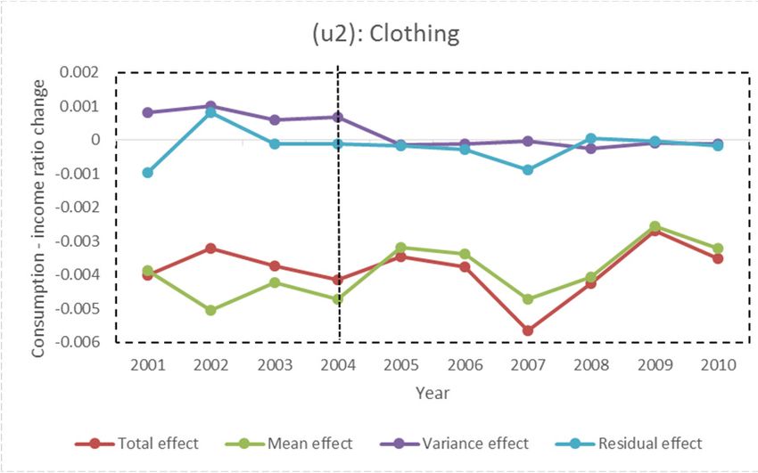
Sustainability 2019, 11, 984                                                                        3 of 22

these have had little effect. So, the main purpose of this paper is to analyze the internal mechanism of
why China’s consumption demand has not fully promoted economic growth.
     Further, in sharp contrast to the lack of consumer demand, there has been a series of consumer
booms in single markets, such as real estate, cars, Apple mobile phones, and other high-tech digital
products, and Chinese consumers have been eager to purchase some goods that are booming
overseas, so inadequate domestic demand is not the whole question; Chinese residents still have
a strong consumer potential. We see a “lack of overall demand but strong local demand” coexistence
phenomenon. So, we believe that there are certainly deeper reasons for the special economic operation
phenomenon caused by the accumulation of deep-seated flaws in China’s economic growth.
     The most direct way to stimulate consumption is to increase residents’ income, but the unequal
promotion will widen the income gap and is not conducive to consumption. The drastic change in
income distribution of billions of people is a significant special factor that distinguishes China from
other countries. The income distribution here refers not only to the income gap that can be expressed
by variances but also to the whole income distribution curve characteristics such as mean, skewness,
and kurtosis. Moreover, the successful experience of Korea and Japan in crossing the “middle income
trap” tells us that the formation of stable, reasonable and strong consumer demand is inseparable
from the sustained growth of household income and reasonable income distribution [5,10]. Therefore,
the final specific research objective is to study the impact of income distribution changes on the
consumption structure.
     Based on the perspective of the income distribution change, this study holds that the above-
mentioned “lack of overall demand, but strong local demand” that coexists with the consumption
structure problem is mainly caused by the imbalance between the demand structure and the supply
structure, and the rapid evolution of the demand structure is the dominant factor in this contradiction.
The effects of the three dynamic characteristics of the income distribution on the consumption demand
structure are called the mean effect, variance effect, and residual effect, respectively. The mean effect
mainly reflects the effect of the overall income level on the whole consumption structure. The variance
effect and the residual effect collectively reflect the effect of the income gap on the consumption
demand. However, the residual effect reflects a symmetry heterogeneity effect that is caused by the
differences of region and human capital. This study calls them “the demand effects of residents’ income
distribution change.”
     In the perspective of income distribution changes, the question of how to expand the domestic
demand and realize the transformation of economic growth driven by consumption is transformed
into the question of how to form a reasonable consumption structure, which is, of course, affected
by the change in the income distribution. Accordingly, once the relationship between the income
distribution and consumption structure is sorted out, the problem of insufficient demand can be
solved at the source, which is of great significance to the structural reform and sustainable growth of
China’s economy.
     The rest of this paper is as follows. The second section is about review of literature. The third
section is the derivation of the AIDS dynamic expansion model. The fourth section is the description
of the data and construction of the indicators; the consumption and income data related to the urban
residents in the Chinese Statistical Yearbook are selected. The fifth section is the empirical test, where
the influence of income changes on the consumption demand structure is measured and discussed.
The sixth Section gives the conclusions and the consequent policy recommendations.

2. Review of Literature
      There are many explanations for the root causes of China’s insufficient domestic demand, and one
of these is the mainstream view that says the problem can be attributed to the Chinese residents’ high
and rising savings. The research [11–13] on this explanation suggests that China’s economic structure
is in rapid change, and the urban and rural social security system is not perfect, so there is uncertainty
about personal future income and expenditure thereby causing residents to require precautionary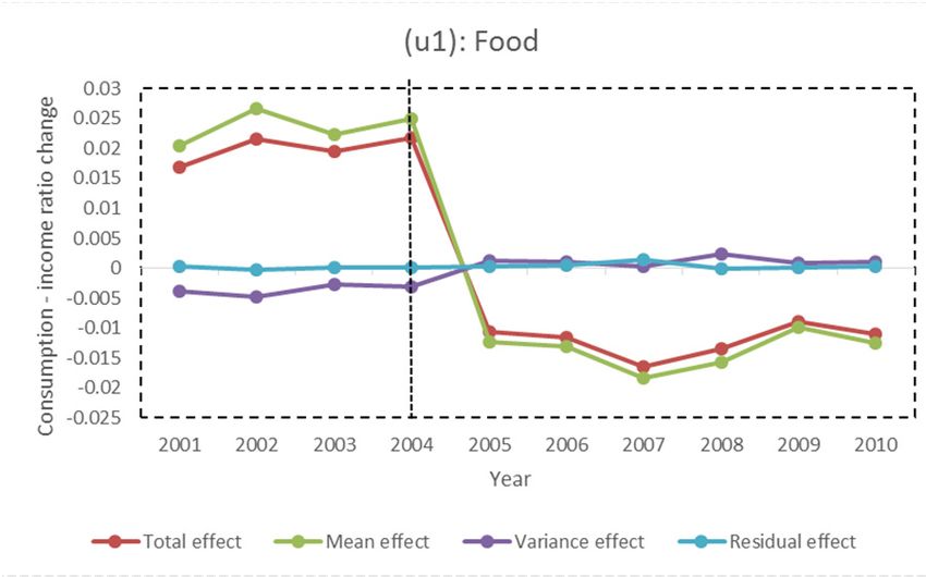
Sustainability 2019, 11, 984                                                                           4 of 22

savings. But Aziz and Cui [14] suggest that the increase in saving alone explains only a small fraction
of the decline in the consumption share; in their view a much larger cause of the problem has been the
role of the declining share of household income in the national income.
      Another popular view is that the insufficient domestic demand is due to the increasing income
disparity between residents, which is actually more a reference to foreign scholars’ related research [15,16].
For example, based on a cointegration and error correction model, Chen [17] found that the urban
Gini coefficient, rural Gini coefficient, and urban and rural income ratio are all Granger reasons for the
decline in the consumption rate. Zhang and Chen [18] used the Theil index to discuss the relationship
between income distribution and expanding domestic demand, and they believe that the widening
income gap is the fundamental factor hindering China’s expansion of domestic demand and the
transformation of economic growth. However, Zhu et al. [19] pointed out that this view is based
solely on the measurement results and lacks sufficient theoretical support, which still needs further
discussion. In recent years some empirical results have also come to the opposite conclusion: Li [20]
studied the relationship between the income gap and consumption demand of urban residents in
China and found that the widening income gap could not be the main cause of the inadequate domestic
demand; Qiao and Kong [21] argued that the impact of the income gap on the consumption propensity
is related to the level of economic development; Su and Sun [22], by depicting the “U” non-linear
characteristics of Chinese residents’ consumption demand with income changes, further argued that
the income gap may not be the main reason for the insufficient domestic demand. From the current
empirical results, this view reflects a certain degree of controversy.
      Theoretically, the view of the income distribution affecting consumption is derived from
Keynes [23], who proposed the rule of the “marginal propensity to decline.” If a social income
distribution gap widens, income will be concentrated in the hands of a small number of people,
and the marginal propensity to consume will lead to a decline in consumer demand. However, this
hypothesis focuses on short-term analysis and does not give sufficient attention to the long-term
relationship between income distribution and consumption demand. In response to this deficiency,
Modigliani proposed a life-cycle hypothesis [24], which argues that consumption depends on the
permanent income not the current income. In the generalized life cycle hypothesis, he also believes
that a widening income gap will lead to a lack of consumer demand through the bequest effect.
Post-Keynesians believe that income distribution is a determinant of consumer demand. They have
established a persuasive theoretical model [25,26] trying to reveal the relationship between income
distribution and consumer demand, and the conclusion is that a widening income gap leads to
insufficient demand.
      In fact, these theories do not show a clear relationship between income distribution or the
income gap and social aggregate demand, because they have all adopted a simplified way of using
“the representative agent” to deal with the problem of aggregation, that is, the transition from the
individual level to macro data. Stokes [27] confirms that the form and coefficient of the macroscopic
consumption function depend not only on the form and coefficient of the microscopic function but
also depend on the characteristics of the social income distribution. Campbell and Mankiw [28] then
broke this homogeneity constraint and put forward the “λ hypothesis.” This hypothesis holds that
a class of consumers in society chooses to consume based on their permanent income, whereas the
other consumers base their consumption on their current income. If you choose to spend based on
your permanent income, the widening income gap will result in a reduction in consumption through
bequests; if the current income is arranged to be consumed, the widening income gap will result in a
reduction in consumption through a reduction in the consumption propensity.
      In addition to the above two points of view, there are still aspects related to the population age
structure and infrastructure that need to be considered [29,30], and it clear that there is no perfect
explanation for the issue of insufficient domestic demand. Although there is little doubt that these
factors could be important in explaining the insufficient domestic demand, it is less convincing that
Sustainability 2019, 11, 984 5 of 22
these are the main reasons because of the incompetence facing the phenomenon of the strong demand
in a single market.
Therefore, China’s domestic demand problem is not just a matter of level, but it is also a structural
problem. There are many explanations for it, but, as we all know, the dramatic changes in the income
distribution have been one of the most significant social characteristics in China [31], and the impact of
income distribution is very important to consumption. Therefore, the idea of analyzing the impact
of changes in income distribution on the evolution of consumption structure arose. Fitting income
distribution is a traditional economic problem, especially in the field of labor economics. Recently,
scholars have paid more attention to the decomposition of income distribution changes in order to dig
deeper information of income changes. Using counterfactual analysis the income distribution can be
decomposed into three parts: the mean change, variance change, and residual (skewness, kurtosis,
and other high-order moments) change [32,33]. This study will also use this method to decompose the
income distribution of Chinese residents. The counterfactual method was first proposed by Fogel [34].
He used it to measure the contribution of the railway to the economic growth of the United States in
the 19th century, refuting the mainstream view that the large-scale railway investment was the main
reason for the rapid growth of the US economy at that time. Today it is still widely used in the impact
assessment of events or policies [35].
Although it is a new attempt to explain the demand of urban residents in China from the
perspective of the income distribution change, the existing research on the consumption structure has
laid a solid foundation for the work in this study. The study of consumption structure began in the
1950s. Subsequently, different models have been proposed one after another. The more famous models
are the linear expenditure system (LES) proposed by Stone [36], the extended linear expenditure
system (ELES) model proposed by Lluch [37], and the approximate ideal demand system (AIDS)
model proposed by Deaton [38]. Among them, AIDS model is the most widely used. Based on this
model, Ray [39] used household expenditure survey data to analyze the consumption structure of
Indian residents, while Blanciforti and Green [40], Chesher and Rees [41] studied the food consumption
situation of American and British residents respectively. Filippini [42] measured the various elasticities
of Swiss household consumption. However, there is a non-linear relationship between the share of
commodity expenditure and the price and expenditure in the AIDS benchmark model. Therefore,
only the non-linear method can be used in the estimation, which makes the actual estimation not
very convenient. Deaton [38] proposed that when the prices of various consumer goods have
strong multi-collinearity, they can be approximated by linear relationship (LA-AIDS). Subsequently,
the expansion of AIDS has gradually enriched, such as inverse AIDS, quadratic AIDS, two-stage linear
expenditure system-approximate ideal demand system LES-AIDS, etc [43–48].
In addition, more and more scholars begin to add some other variables to traditional AIDS
or LA-AIDS models, such as demographic characteristics, seasonal variables, time trend variables,
structural change paths, and other external disturbances, to characterize the impact of these factors on
budget share and consumption structure [40,49]. These studies make the AIDS model more perfect
and convenient. Therefore, this paper also chooses AIDS model as the basic model to integrate the
factors of income distribution changes.
However, numerous existing AIDS models are all based on the assumption that the expenditure
is equal to the income; the expenditure is allocated among the different commodities, and then the
expenditure structure is used to approximate the demand structure. Foreign economic development
tends to be stable, because the residents’ income is already at a high level, and the credit and social
security systems are perfect. In these circumstances the residents have the courage to advance their
consumption, and the expenditure structure can then better reflect the demand structure.
China’s economy is operating at a rapid speed, the residents’ income changes violently, and the
rapid and significant change in income of hundreds of millions of people has a strong impact on
consumer demand, which is rarely encountered in the development of other countries. Coupled with
the lack of social security and the consumption habit of “base one’s expenditures upon one’s income”Sustainability 2019, 11, 984 6 of 22
and other reasons, a considerable part of the residents’ income is saved, so their expenditure is not
equal to their income, and then the expenditure and demand structures are inconsistent. Therefore,
to study China’s consumption structure problem, following the existing foreign models will require
some deviations.
In order to achieve the research objectives, this study will make two improvements to the AIDS
model. One of these is to relax the hypothesis that the expenditure is equal to the income through the
introduction of income items in the model to make it more in line with the concept of consumption of
China’s residents. The second improvement to the AIDS model is based on counterfactual analysis,
whereby the three dynamic features of the income distribution change are introduced into the model.
3. Construction of the Model Used
In order to study the imbalance of the consumption structure from the perspective of the income
distribution, we need to expand the AIDS model. The AIDS model is to achieve the established utility
level by minimizing the expenditure, and the Hicks demand function is obtained. By solving the
duality problem of the AIDS model, the Marshallian demand function is solved according to the utility
maximization principle under the budget constraint condition so the model contains the revenue items
that can reflect the characteristics of the Chinese residents’ consumption. The dynamic characteristics
of the changes in the income distribution of the residents are then quantified; this part mainly draws
on the research of Jenkins and Van Kerm [33]. After completing the decomposition of the change in the
income distribution, the income distribution characteristic is introduced into the model by means of
an anti-fact process.
3.1. The Duality Problem of the AIDS Model
The AIDS model assumes that the consumer behavior satisfies the price indifferent generalized
logarithmic preference hypothesis, so the expenditure function is
ln(C (u, p)) = (1 − u) ln( a( p)) + u ln(b( p)), (1)
where u(0 ≤ u ≤ 1) is the utility index, u = 0 only to maintain the basic physiological needs of
the utility, and u = 1 for the utility to achieve its maximum. a( p) and b( p) denote the minimum
expenditure required by the consumers to meet their basic physiological needs and obtain the
maximum utility, and the form is as follows:
n n n
1
ln( a( p)) = a0 + ∑ ai ln( pi ) + ∑ ∑ rij ln( pi ) ln( p j ),
2
i =1 i =1 j =1
n , (2)
ln(b( p)) = ln( a( p)) + b0 ∏ pi bi
i =1
According to the principle of duality, the expenditure function and indirect utility function are
inverse functions, so the indirect utility function corresponding to the expenditure function is
v( p, m) = (ln m − ln a( p))/(ln b( p) − ln a( p)), (3)
As obtained from the Roy equation, the Marshallian demand function for the commodity i is
n
xi ( p, m) = −[∂v( p, m)/∂pi ]/[∂v( p, m)/∂m] = (m/pi )( ai + ∑ rij∗ ln( p j ) + bi ln(m/a( p))), (4)
j =1Sustainability 2019, 11, 984 7 of 22
where rij∗ = (rij + r ji )/2. Given µi = pi xi ( p, m)/m represents the ratio of the expenditure to income
for commodity i, we get an expanded version of the AIDS model with income m as follows:
n
µi = ai + ∑ rij∗ ln( p j ) + bi ln(m/a( p)), (5)
j =1
If we take the difference between the income and expenditure as savings, this can be seen as a
special commodity that buys a certain amount of vouchers for future consumption. Let the discount
rate 1/(1 + r ) be the price of the savings, where r is the real interest rate. To preserve the aggregation
n n n
properties of AIDS, this is ∑ ai = 1, ∑ rij∗ = 0, ∑ bi = 0. Furthermore, a( p) can be understood as
i =1 i =1 i =1
a price index, so it can be set to a( p) ≈ θP, where P is the total price index. We take it into the
Equation (5), then
n
µi = ai∗ + ∑ rij∗ ln( p j ) + bi ln(m/P), (6)
j =1
where ai∗ = ai − bi ln θ, and it also satisfies the aggregation property. Moreover, Equation (6) also
n
satisfies the homogeneity ∑ rij∗ = 0 and the symmetry rij∗ = r ∗ji .
j =1
3.2. Counterfactual Decomposition of Income Distribution
Before the AIDS model is dynamically expanded, we should complete the measurement of the
income distribution changes. For the decomposing method of the income distribution, by using a
counterfactual analysis method, Jenkins and Van Kerm [33] successfully decomposed the income
distribution change into three parts, which reflect the mean, variance, and residual changes. In fact,
the residual change reflects the skewness, kurtosis, and other high-order moments changes of the
income distribution. Counterfactual analysis can be understood as an application of comparative static
analysis, a qualitative research method in economics. The difference is that counterfactual analysis is a
quantitative analysis method. It constructs a counterfactual situation in which only one factor changes
but other factors remain unchanged relative to a basic fact. And it evaluates the impact of a single
factor by comparing the results of counterfactual and factual situations based on specific regression
models or statistical methods., so we will use the counterfactual decomposition method of Jenkins and
Van Kermin in this study.
Suppose that we have and y2 for two years of the income survey data, assuming we temporarily
disregard the price factors and they follow the same distribution, y1 ∼ F (µ1 ,σ1 2 ) and y2 ∼ F (µ2 ,σ22 ),
then the decomposition process can be illustrated below:
meanchange variancechange residualchange
y1 (µ1 , σ12 ) → ξ 1 ∼ F (µ2 , σ12 ) → ξ 2 ∼ F (µ2 , σ22 ) → y2 (µ2 , σ22 ), (7)
Assuming there is only a change in the mean between the two income samples, and then the
underlying income ξ 1 relative to the base period y1 can be denoted by
ξ 1 = y1 + ∆y = y1 + (µ2 − µ1 ), (8)
The variance change reflects the polarization of the income between the individuals around the
mean. Based on the counterfactual analysis, we keep the mean of the counterfactual income ξ 1 and ξ 2
qual and only allow their variance changes. According to the statistical knowledge it is easy to see that
(ξ 1 − µ2 )/σ1 = (ξ 2 − µ2 )/σ2 ∼ F (0, 1). (9)
So we get
ξ 2 = µ2 + σ2 (ξ 1 − µ2 )/σ1 . (10)Sustainability 2019, 11, 984 8 of 22
The difference between ξ 2 and y2 is the residual change.
3.3. Dynamic Expansion of AIDS Model
Equation (6) is a static model, but the change in the income distribution is a dynamic process, so
the combination of the two will also be a dynamic system. Based on model (6), the expenditure share
µi of the commodity i can be regarded as a function of the income m and the price vector p, which is
µi (m, p); if p is kept constant, µi (m, p) is similar to the Engel equation of commodity i. Taking the two
periods as an example, the evolution of the consumption structure caused by the income changes can
be decomposed as follows:
µ (y , p ) price→
e f f ect
ηi1 = µi (y1 , p2 )
i1 1 1
, (11)
η = µ (y , p ) mean→ e f f ect
ηi2 = µi (ξ 1 , p2 )
variance e f f ect
→ ηi3 = µi (ξ 2 , p2 )
residual e f f ect
→ µi2 (y2 , p2 )
i1 i 1 2
The above process is clearly also a counterfactual decomposition process and its first step is to
eliminate the impact of the price change. The mean, variance, and residual effects of the evolution of
the consumption structure caused by income distribution change are then denoted by ∆1 , ∆2 , and ∆3 ,
respectively. So,
∆1 = ηi2 − ηi1 = αi ln(ξ 1 /y1 )
∆2 = ηi3 − ηi2 = β i ln(ξ 2 /ξ 1 ) (12)
∆3 = µi2 − ηi3 = θi ln(y2 /ξ 2 )
Then, the dynamic expansion model of AIDS can be obtained as follows:
µi2 = ηi1 + ∆1 + ∆2 + ∆3
n
(13)
= ai∗ + ∑ rij∗ ln( p j2 ) + bi ln(y1 /p2 ) + αi ln(ξ 1 /y1 ) + β i ln(ξ 2 /ξ 1 ) + θi ln(y2 /ξ 2 )
j =1
Equation (13) is the dynamic expansion of the AIDS model, which includes the factors of the
income distribution change. The dependent variable is the consumption share of each commodity
in the second period, and the independent variable contains two kinds of price factors and income
distribution factors: ∑nj=1 rij∗ ln( p j2 ) denotes the impact of its own price and the interactive price,
and ln(y1 /p2 ) represents the change in real income due to the price changes. These factors measure
the effect of the price on various expenditures together, as the nominal income remains constant.
Obviously, the three items ln(ξ 1 /y1 ), ln(ξ 2 /ξ 1 ), and ln(y2 /ξ 2 ) indicate the impact of the changes in
the income distribution, which is the focus of this study.
4. Data Preparation and Regression Equation Setting
4.1. Data Preparation
The focus of this study is to examine the issue of China’s domestic demand, not the dynamic
evolution trend of the consumption structure. As can be seen from the consumption rate curve in
Figure 1 (source: [1]), the significant decline in consumption rate occurred between 2000 and 2010
is what we want to explain from the structural level. In addition, as China’s economy enters a new
normal, the statistical caliber of urban residents’ income has also changed since 2012. After 2010, only
two years of data are available. For the robustness of the results, the empirical discussion focuses on
the provincial panel data from 2000 to 2010.Sustainability 2019, 11, 984 9 of 22
Sustainability 2018, 10, x FOR PEER REVIEW 9 of 22
Figure 1. Consumption Rate of Chinese Urban Residents during 1995–2014.
Figure 1. Consumption Rate of Chinese Urban Residents during 1995–2014.
The data used are mainly from the National Statistical Yearbook 2000-2010 data in respect of
For the
the urban income indexes,
residents which are The
in the provinces. the last three income
indicators items inthe
used include model (13), the structure
expenditure data for of the
eight
two potential income variables and are relative to the income of the
categories of goods, the disposable1income2data, the classified consumer price index, and the annual previous year, so the
change in
nominal the income
interest distribution
rate data. The eightiscategories
measuredofbetweengoods arethefood,
adjacent two residence,
clothing, years. Thehousehold
standard
deviation will be used when we calculate ;
facilities, medical care, transportation and communications,
2 the income data of the yearbook are derived
entertainment and education, and from the
other
same household
miscellaneous surveyand
expenses data, so theThe
services. standard
nominaldeviation is calculated
interest rate by using
used is a 1-year the data
time deposit of which
rate, seven
income
is levels
actually in each year,
the average annualand the proportion
interest rate. Because of the
thepopulation
government inonly
eachannounces
group is 0.1,
the0.1, 0.2, 0.2, 0.2,
corresponding
0.1, and rate
interest 0.1, respectively (see Table
of the adjustment 1).there are multiple interest rates in a given year, this study will
day, if
average the different interest rates by the number of days. In addition, we still need to construct some
new indicators based onTable 1. Disposable
the available data.Income of Chinese Residents by Group.
ForPer
thecapita
income indexes, which areLower the last three income items in model (13), the structure
Upper of the
Standard
Year
two potential Lowest Low
income variables ξ 1 and Middle Middle
ξ 2 are relative to the income High Highest
income Middle of the previous year, so deviation
the change
in2000
the income6280.0distribution
2653.0 is measured
3633.5 between the
4623.5 adjacent
5897.9 two years.
7487.4 The standard
9434.2 13,311.0 deviation
1122.7will
be2001
used when6859.6 2802.8 ξ 23319.7
we calculate ; the income 4946.6
data of6366.2
the yearbook8164.2 12,662.6
are derived from15,114.9 1424.4
the same household
2002 7702.8 2408.6 3032.1 4932.0 6656.8 8869.5 15,459.5
survey data, so the standard deviation is calculated by using the data of seven income levels 18,995.9 1919.1
in each
2003 8472.2 2590.2 3295.4 5377.3 7278.8 9763.4 17,471.8 21,837.3
year, and the proportion of the population in each group is 0.1, 0.1, 0.2, 0.2, 0.2, 0.1, and 0.1, respectively 2224.4
2004
(see Table 9421.6
1). 2862.4 3642.2 6024.1 8166.5 11,050.9 20,101.6 25,377.2 2609.4
2005 10,493.0 3134.9 4017.3 6710.6 9190.1 12,603.4 22,902.3 28,773.1 2988.4
2006 11,759.5 3568.7 4567.1
Table 1. 7554.2
Disposable Income10,269.7
of Chinese 14,049.2 25,410.8
Residents by Group. 31,967.3 3303.3
2007 13,785.8 4210.1 6504.6 8900.5 12,042.3 16,385.8 22,233.6 36,784.5 3406.6
2008 15,780.8
Per Capita 4753.6 7363.3 10,195.6
Lower 13,984.2 19,254.1
Upper 26,250.1 43,613.8 Standard
4087.8
Year Lowest Low Middle High Highest
2009 Income 5253.2
17,174.7 8162.1 Middle 15,399.9
11,243.6 Middle
21,018.0 28,386.5 46,826.1 Deviation
4366.2
2010
2000 19,109.4
6280.0 5948.1
2653.09285.3
3633.5 12,702.1
4623.5 17,224.0
5897.9 23,188.9
7487.4 31,044.0
9434.2 51,431.6
13,311.0 4750.0
1122.7
2001
Note: The 6859.6 2802.8
per capita income 3319.7
data are 4946.6 and 6366.2
not calculated 8164.2
are the original data in12,662.6 15,114.9Yearbook.
the China Statistical 1424.4
All
2002 7702.8 2408.6 3032.1 4932.0 6656.8 8869.5 15,459.5 18,995.9 1919.1
data were converted using 2000 as the base year.
2003 8472.2 2590.2 3295.4 5377.3 7278.8 9763.4 17,471.8 21,837.3 2224.4
2004
For the9421.6 2862.4
price indicators 3642.2
we use6024.1 8166.5
the 2000–2010 11,050.9 20,101.6
consumer 25,377.2for the
price indices 2609.4
various
2005 10,493.0 3134.9 4017.3 6710.6 9190.1 12,603.4 22,902.3 28,773.1 2988.4
commodities
2006
based on 2000.
11,759.5 3568.7
We4567.1
take the7554.2
discount10,269.7 + r) as the
rate 1 (114,049.2 price of31,967.3
25,410.8
the savings,3303.3
where the
real 2007
interest 13,785.8
rate r is obtained
4210.1 by using8900.5
6504.6 the annual nominal
12,042.3 interest
16,385.8 rate minus
22,233.6 the total3406.6
36,784.5 consumer
price2008
index. 15,780.8
In order to 4753.6
maintain7363.3 10,195.6
the order 13,984.2 consistent
of magnitude 19,254.1 26,250.1 43,613.8
with the other 4087.8 price
commodity
2009 17,174.7 5253.2 8162.1 11,243.6 15,399.9 21,018.0 28,386.5 46,826.1 4366.2
indices,
2010 the savings
19,109.4 price is also9285.3
5948.1 converted at the17,224.0
12,702.1 2000 base23,188.9
price. The total price
31,044.0 index also
51,431.6 needs to
4750.0
be reconstructed assuming that the share of savings is s, then the "total price index = (1 − s) total
Note: The per capita income data are not calculated and are the original data in the China Statistical Yearbook.
expenditure price
All data were converted + s savings
index using 2000 as theprice index."
base year.
4.2. Regression Equation
For the price Setting
indicators we use the 2000–2010 consumer price indices for the various commodities
basedWith
on 2000. We take
the rapid the discount
economic rate
growth, 1/(1 + rliving
residents’ ) as thestandards
price of the savings,
have wheregreat
undergone the real interest
changes, so
rate r is obtained by using the annual nominal interest rate minus the total consumer price index.
the consumer spending structure is bound to change significantly as a consequence of this. Therefore,
the problem of structural mutation must be considered when we estimate the model. In order toSustainability 2019, 11, 984 10 of 22
In order to maintain the order of magnitude consistent with the other commodity price indices,
the savings price is also converted at the 2000 base price. The total price index also needs to be
reconstructed assuming that the share of savings is s, then the “total price index = (1 − s)× total
expenditure price index +s× savings price index.”
4.2. Regression Equation Setting
With the rapid economic growth, residents’ living standards have undergone great changes, so the
consumer spending structure is bound to change significantly as a consequence of this. Therefore, the
problem of structural mutation must be considered when we estimate the model. In order to avoid
the estimated error caused by the artificial set of abrupt points, this study chooses to use Hansen’s
threshold method to find the abrupt points [50–52], which is completely determined by the data, so we
introduce dummy variables in model (13) as Hansen did. The equation for setting a single mutation
point is as follows:
n
µit = ∑ rij∗ ln( p jt ) + bi ln(yt−1 /pt ) + [ ai1
∗ + α ln( ξ /y
i1 1t t−1 ) + β i1 ln( ξ 2t /ξ 1t ) + θi1 ln( yt /ξ 2t )] · h1 ( t < T )
j =1 (14)
∗ + α ln( ξ /y
+[ ai2 i2 1t t−1 ) + β i2 ln( ξ 2t /ξ 1t ) + θi2 ln( yt /ξ 2t )] · h2 ( t ≥ T )
where T is the structural break point, h1 (t < T ) and h2 (t ≥ T ) are both indicator functions. If t < T,
then h1 = 1, and h2 has a similar definition. This study only adds the dummy variable to the intercept
term and the income change factor; the price variable is not the focus, so we take it as the control
variable. Because of the use of the panel data, the equation intercept also introduces province dummy
variables to remove the impact of the individual effects, which is not reflected in the equation.
When the structural mutation is not considered, the degree of freedom of the system is 92, so in
order to ensure the robustness of the estimation results, the time interval span set in this study is not
less than three years. The sample point for each year is 31, which ensures that there are no less than 93
data observations per interval. Therefore, the potential mutation points considered in this study are in
the 2003–2007 range. In addition, Hansen chooses the residual squared sum as the criterion of fitting
and then determines the mutation point, and this study chooses the logarithmic maximum likelihood
statistic in the regression result. The larger the likelihood value, the more likely that the corresponding
potential mutation year is real.
From the above results (Table 2), the corresponding logarithmic likelihood is largest in 2004, and
the results of the likelihood ratio test show that the original hypothesis of structural change is rejected
at the significance level of 1%, so the structural mutation point T is 2004. So far, the final regression
equation used in this study has been obtained.
Table 2. (a, b) Determination of the Point of Structural Change.
(a)
Mutation Point 2003 2004 2005 2006 2007
Likelihood Value 9033.876 9035.975 * 9035.189 9001.732 8980.904
(b)
Critical value
Likelihood-ratio Test Test Statistic df Probability
1% 5% 10%
Assumption: No
250.20 32 0.000 53.486 46.194 42.585
Structural Change
Note: (a) Tests of potential mutation years, (b) Nonlinear test with 2004 as the mutation year. * indicates that
the value is the largest. The “df” is the degree of freedom and the likelihood-ratio test is based on the results of
Table 2(a).Sustainability 2019, 11, 984 11 of 22
5. Empirical Results and Discussion
5.1. The Counter-factual Decomposition of Income Distribution
From the non-parametric kernel density estimation results of the residents’ income distribution
(Figure 2, source: [1]), we can see that the income level and the income gap have both changed
significantly, and the domestic scholars Sun and Su [31] show that the growth in the income level is
dominant. Therefore, if we do not consider the growth in income when discussing the lack of demand,
Sustainability
is bound 2018,
itSustainability to 10, x FOR PEER
exaggerate REVIEW impact of the income gap and thereby add fuel to the controversy
the negative 11 of 22
2018, 10, x FOR PEER REVIEW 11 of 22
mentioned earlier.
.0004
.0004 INC_1997 Kernel INC_1998 Kernel
INC_1999
INC_1997 Kernel
Kernel INC_2000
INC_1998 Kernel
Kernel
INC_2001
INC_1999 Kernel
Kernel INC_2002
INC_2000 Kernel
Kernel
INC_2003
INC_2001 Kernel
Kernel INC_2004
INC_2002 Kernel
Kernel
INC_2005
INC_2003 Kernel
Kernel INC_2006
INC_2004 Kernel
Kernel
.0003 INC_2007
INC_2005 Kernel
Kernel INC_2008
INC_2006 Kernel
Kernel
.0003 INC_2009
INC_2007 Kernel
Kernel INC_2010
INC_2008 Kernel
Kernel
INC_2011
INC_2009 Kernel
Kernel INC_2012
INC_2010 Kernel
Kernel
INC_2013
INC_2011 Kernel
Kernel INC_2014
INC_2012 Kernel
Kernel
Density
INC_2013 Kernel INC_2014 Kernel
Density
.0002
.0002
.0001
.0001
.0000
.0000 0 10,000 20,000 30,000 40,000
0 10,000 20,000 30,000 40,000
Income .
Income .
Non-parametric
Figure2.2.Non
Figure - parametricKernel
Kernel Density
DensityEstimation
EstimationResults
Resultsof
ofIncome
IncomeDistribution.
Distribution.
Figure 2. Non - parametric Kernel Density Estimation Results of Income Distribution.
Based on the counter-factual decomposition method of Jenkins and Van Kerm [33], the non-
Based on the counter-factual decomposition method of Jenkins and Van Kerm [33], the non-
Based kernel
parametric on the density
counter-factual decomposition
decomposition is estimatedmethod
for of
theJenkins anddisposable
per capita Van Kerm income
[33], theofnon-
the
parametric kernel density decomposition is estimated for the per capita disposable income of the
parametric kernel density decomposition is estimated for the per capita disposable income
urban residents in 30 provinces. The results of the decomposition of the income distribution between of the
urban residents in 30 provinces. The results of the decomposition of the income distribution between
urban
the residents
other in 30are
two years provinces. Thesoresults
consistent, of the
we only take decomposition
the 2005–2006ofgroup
the income
in the distribution
middle of the between
study
the other two years are consistent, so we only take the 2005–2006 group in the middle of the study
the other
period two
as an years are
example consistent,
(Figure 3). Theso we only
graph takeform
is in the the 2005–2006 group
of a probability in thecurve,
density middle of the
which is study
fitted
period as an example (Figure 3). The graph is in the form of a probability density curve, which is
period as an example (Figure 3). The graph is in the form
according to the counter-factual income variables of each province. of a probability density curve, which is
fitted according to the counter-factual income variables of each province.
fitted according to the counter-factual income variables of each province.
Figure 3. Decomposition of Income Distribution Changes during 2005–2006.
Figure 3. Decomposition of Income Distribution Changes during 2005–2006.
Figure 3. Decomposition of Income Distribution Changes during 2005–2006.
From the results we can see that the mean change is the dominant effect, the variance change is the
From thedominant
second-most results we can see
effect, andthat
the the meanchange
residual change is thesmallest.
dominant effect, the variance change is
From the results we can see that the mean changeisisthe
the dominant Furthermore, the mean
effect, the variance change
change is
the
is second-most
basically alwaysdominant
consistent effect, and
with and the
the total residual change
change, change is the
whereasisthe smallest. Furthermore, the mean
the second-most dominant effect, the residual thevariance
smallest.and the residual
Furthermore, thechange
mean
change
are is basically
opposite always
to the mean consistent
change beforewith the 11910,
income total change, whereaswith
then consistent the variance
the meanand the residual
change, and the
change is basically always consistent with the total change, whereas the variance and the residual
change
residual are opposite
change is to the
slightly mean
ahead change
of the before
varianceincome 11910,
change. It canthen
be consistent
speculated with
that the
if mean
the change,
shortage of
change are opposite to the mean change before income 11910, then consistent with the mean change,
and the residual change is slightly ahead of the variance change. It can be speculated that if the
and the residual change is slightly ahead of the variance change. It can be speculated that if the
shortage of domestic demand is indeed caused by the income factors, focusing only on the income
shortage of domestic demand is indeed caused by the income factors, focusing only on the income
gap may not be comprehensive, because it is not the main feature of the income distribution changes.
gap may not be comprehensive, because it is not the main feature of the income distribution changes.
Therefore, it is necessary to rethink the problem from the whole feature of the change in the income
Therefore, it is necessary to rethink the problem from the whole feature of the change in the income
distribution.
distribution.Sustainability 2019, 11, 984 12 of 22
domestic demand is indeed caused by the income factors, focusing only on the income gap may not be
comprehensive, because it is not the main feature of the income distribution changes. Therefore, it is
necessary to rethink the problem from the whole feature of the change in the income distribution.
5.2. Model Estimation Results and Analysis
The model we used is a system, and each equation does not contain endogenous explanatory
variables. If we ignore the correlation between the disturbance terms of the different equations,
the ordinary least squares estimate for each equation is consistent but not the most efficient. There is
likely to be a period correlation between the residents’ different expenditures, so it is efficient to use
the Seemingly Unrelated Regression (SUR) to estimate the entire system at the same time. In addition,
since the dependent variable of each equation is the proportion of “consumption expenditure/income,”
the sum is 1. In order to avoid over-recognition of the model estimation, one equation must be
removed. Theoretically, randomly removing any one does not affect the result, and the parameters of
the removed equation can be calculated through the constraints. But the purpose of this study is mainly
to examine the impact of the income distribution changes on the consumption structure, and savings
exists more as a tool variable, so choosing to remove the savings equation and its estimated results
will not be given. For the parameter estimates, only the coefficient estimates of ln(ξ 1 /y1 ), ln(ξ 2 /ξ 1 )
and ln(y2 /ξ 2 ) representing the income distribution change are given.
From the estimation results (Table 3), the model is well fitted, the Root Mean Square Error (RMSE)
of each equation is small, and all R-square values are greater than 0.97. Furthermore, the correlation
between the perturbations of the equations have also been tested by the Breusch-Pagan test, and the
last line of Table 3 shows that the p-value of the “no-period correlation” is 0, so the original hypothesis
of “the disturbance term is independent” can be rejected at a significance level of 1%. Therefore, the use
of SUR for the systematic estimation can improve the estimation efficiency.
Table 3. The Estimation of the Impact of Income Distribution on the Consumption Structure.
Period Effects (u1) (u2) (u3) (u4) (u5) (u6) (u7) (u8)
0.219** −0.00415 0.00676 −0.333*** 0.113*** 0.306*** 0.278*** −0.418***
2000–2004
Mean
(2.52) (−0.80) (0.11) (−6.75) (2.76) (3.90) (4.56) (−11.68)
0.266*** −0.0576 −0.0357 -0.0626* 0.108*** 0.0536 0.142*** −0.138***
Variance
(4.02) (−1.46) (−0.73) (−1.66) (3.43) (0.89) (3.00) (−5.23)
−0.0321 −0.0838*** −0.0465* 0.0166 0.0380** 0.0101 0.0135 −0.00973
Residual
(0.90) (−3.92) (−1.76) (0.83) (2.25) (0.31) (0.53) (−0.66)
−0.106*** −0.0274 −0.0400 −0.0142 −0.0350** −0.0504* −0.0100 0.0203
2005–2010
Mean
(−3.28) (−1.37) (−1.59) (0.74) (−2.17) (−1.65) (−0.42) (−1.55)
−0.125** 0.0128 −0.125*** 0.0318 −0.0508* 0.0308 0.0946** 0.0966***
Variance
(−1.98) (0.35) (−2.67) (0.91) (−1.70) (0.55) (2.14) (3.94)
−0.0626* 0.0378* −0.0522** 0.00428 −0.0111 0.0234 0.0353 0.0319**
Residual
(−1.76) (1.79) (−2.00) (0.22) (−0.66) (0.73) (1.41) (2.17)
RMSE 0.0105 0.0061 0.0075 0.0057 0.0047 0.0094 0.0071 0.0042
“R-sq.” 0.9986 0.9946 0.9905 0.9858 0.9928 0.9887 0.9948 0.9795
Breusch-Pagan test of independence: chi2(28) = 174.237, Pr = 0.0000
Note: The t statistics are in parentheses. The symbols and thresholds are * for p < 0.1, ** for p < 0.05, and ***
for p < 0.01. “R-sq” represents R-squared statistics. (u1)–(u8) represent eight categories of goods: (u1) food, (u2)
clothing, (u3) residence, (u4) household facilities, (u5) medical care, (u6) transportation and communications, (u7)
entertainment and education, and (u8) other miscellaneous expenses and services.
For the period 2000–2004, the impact of the mean effect on clothing and residential consumption
is not statistically significant. Among the consumption items that are significantly affected by the
change in the mean of the income distribution, there is a positive impact on the consumption of food,
medical care, transportation, entertainment, and education, and a negative impact on consumption
of household equipment and miscellaneous services. We know that the demand for basic living
expenses for food, clothing, and household equipment in China had been basically met by the year
2000 as a result of the rapid increase in the overall income level of the residents. According to theSustainability 2019, 11, 984 13 of 22
data in the 2001 China Statistical Yearbook, by the end of 2000 the three sets of traditional home
appliances, TV sets, washing machines, and refrigerators, had reached a high level of 116.56 units,
90.52 units, and 80.13 units per 100 urban residents. Therefore, during this period the proportion of
household consumption expenditure on household equipment decreased with the increase of income,
thereby reflecting the “Engel Law” trend. The positive effect of the mean change on food expenditure
shows that the dietary structure of Chinese residents in this period was further optimized; people
not only took “eat full” as a standard, more and more chose to pursue the “eat good” policy with
an improvement in their food quality, and the proportion of spending on dining outside the home
also increased. The trend with clothing expenditure is just between the middle of the two types of
goods. The proportion of the expenditure on clothing is not sensitive to the growth of the income level,
indicating that the residents’ basic needs have been met, but the pursuit of quality has not yet been
reflected. During this period, residents mainly focused on the three “core consumption” categories,
which are health care, transportation and communications, and entertainment and education. This
consumption structure represents a transition from a basic one to a development-centric one, but the
enjoyment-centric consumption represented by the “other miscellaneous expenses and services” had
not yet attracted the attention of the urban residents in the short term; they chose to reduce the basic
type of consumption and transfer their focus onto the development-centric consumption.
China’s income distribution is obviously right-sided, with the high-income groups growing
rapidly, so the variance effect and residual effect mainly represent changes in the consumption choices
of the high-income earners. The variance effect for the period 2000–2004 has a significant positive
effect on the consumption of food, medical care, culture, and education, whereas it has a significant
inhibitory effect on household facilities and miscellaneous services and has no significant effect on
other items. This indicates that the high-income group will further increase their share of expenditure
on food, medical care, and cultural education. As their income grows at a relatively faster pace, more
income will be used to enjoy higher quality food and health care services and to receive better quality
education, which may enhance their individual heterogeneity advantages and help them to stay in
the forefront in terms of income distribution. However, the expenditures on household equipment,
tourism, and other miscellaneous services have also been reduced, which may have been caused by
a lack of innovation in the home appliance industry and the immaturity of the tertiary industry at
that time.
The residual effect reflects the choice of the consumers with the most heterogeneous advantage,
whose position in the income distribution levels was relatively higher. During 2000–2004 the residual
effect had no significant effect on the other items except that there was a significant negative impact
on the consumption of clothing and housing and a positive effect on the consumption of health
care. As they are the group with the fastest growing income, they are most concerned about medical
expenses and may even sacrifice some short-term clothing and residential consumption to meet their
medical expenses. The difficult problem of seeing a doctor was always the focus of the society’s
attention in this period.
During 2005–2010 the mean effect had a significant negative effect on food, health care, and
transportation, but the impact on the other categories of consumption was not significant. Therefore,
compared with 2000–2004, the positive pull impact of the mean effect on the consumption rate
disappeared, which perhaps just reflects the problem of the continuing decline of China’s consumption
rate with the mean effect reflecting the consumption dynamics of the main body of society. Fortunately,
the variance and residual effects reflect some positive effects on individual markets, such as the variance
effects on the expenditure on cultural and educational activities and miscellaneous services, and the
residual effects on clothing and other services, even though their negative impacts on certain markets
still exist. Based on the results, first, the second round of household food consumption has been
completed, so the three effects of the income distribution are negative. Second, thanks to the deepening
of the health care reform since 2005, which was defined as “The Year of Hospital Management” by
the government, the medical expenses proportion of income has been reduced significantly. Finally,Sustainability 2019, 11, 984 14 of 22
the trend of further escalation of the consumption structure is beginning to emerge, which shows
that families with faster income growth tend to increase their spending on education and services.
In addition, the attitudes towards apparel consumption have changed with people beginning to focus
more on the quality and brand of clothing.
Considering the importance and centrality of real estate to China’s economy, the issue of
residential consumption will be discussed separately here. The results of Table 3 show that the
mean effect of the two periods both had no significant effect on the residential consumption. The
variance effect was not significant before 2004 but began to show a significant negative effect after
2004, while the residual effect reflects the negative impact on the consumption devoted to living
expenses in the two periods. It is easy to understand why the mean effect is not significant, and this is
because since 1998 the implementation of housing distribution monetization replaced the previous
housing in-kind distribution. China’s housing prices began to rise, especially in 2000–2010, which is
known as the “Golden Decade” of the real estate market. Under the continued rising expectations,
the housing bubble continued to expand, and according to the statistics of the Chinese Academy of
Social Sciences in 2004, in Beijing and Shanghai the overall household debt ratio, which reached 155%
and 122%, respectively, was higher than the ratio for European and American families. Therefore, with
the investment attributes of the house becoming stronger, the residential market has gradually moved
out of line with the income levels, and the mean effect has lost its role.
It is contrary to our intuition that the residual effect in the first period and the variance and
residual effects in the second period have shown a negative impact on residential consumption,
because most people would think that high-income people are characterized by residual and variance
changes and should have increased their living expenses. To understand the statistical content of
the Chinese Bureau of Statistics in respect of the consumption on living expenses, we find that most
of the statistics use costs for the items including housing and decoration materials, rent, mortgage
payments, daily energy consumption, and maintenance, but the expected income from that investment
that should be taken into consideration is not included. For example, renovation costs that are incurred
are included in the statistics reported, and generally Chinese families that are home owners choose
to decorate the house they live in, but they do not decorate it for speculative reasons. Therefore,
in the context of the increasing investment demand for houses, the complementarity between the
usage cost and the housing expenditure is gradually weakened, and the substitution characteristics are
gradually reflected. A few high-income families characterized by residual change chose speculative
living expenses in 2001–2004, while in 2005–2010 the majority of high-income groups characterized
by the variance effect were also involved, thereby strengthening the negative impacts of residual and
variance effects on residential consumption.
In summary, the above model estimates are statistically significant, and they are consistent with
the actual situation that prevailed in China over that time. The consumption effect of the income
distribution in the two periods is obviously different. The mean effect is the theme during 2001–2004,
and the change of the consumption structure from a survival mode to a development mode is the
mainstream. However, the mean effect during 2005–2010 is no longer significant with the overall
consumption being weak. Fortunately, in the individual markets, with regard to the high-income
groups, the variance and residual effects reflect their positive side, which strengthened the individual
market demand, and the consumption structure also shows signs of further escalation.
5.3. Quantitative Counterfactual Estimation of the Effects
The preceding analysis is qualitative, but as is customary in studies of the consumption structure,
quantitative elastic analysis is still needed. However, after introducing the income distribution
variables into the AIDS model, the economic meaning of the variables that this study is concerned
with becomes difficult to define when performing elasticity analysis, especially the interpretation of
the variance and residual terms. Therefore, we have decided to abandon the elasticity analysis and
directly use the previous counterfactual analysis framework and the model’s estimation results toYou can also read