Superconductivity with excitons and polaritons: review and extension - SPIE Digital ...
←
→
Page content transcription
If your browser does not render page correctly, please read the page content below

Superconductivity with excitons and
                polaritons: review and extension

                Fabrice P. Laussy
                Thomas Taylor
                Ivan A. Shelykh
                Alexey V. Kavokin

Downloaded From: https://www.spiedigitallibrary.org/journals/Journal-of-Nanophotonics on 18 Sep 2021
Terms of Use: https://www.spiedigitallibrary.org/terms-of-use
Superconductivity with excitons and polaritons:
                                                     review and extension

                                             Fabrice P. Laussy,a,b Thomas Taylor,a Ivan A. Shelykh,c,d
                                                             and Alexey V. Kavokina,e
                                   a
                                    University of Southampton, School of Physics and Astronomy, Highfield, Southampton,
                                                                     SO17 1BJ, United Kingdom
                                                                      fabrice.laussy@gmail.com
                                    b
                                      Technische Universität München, Walter Schottky Institut, Am Coulombwall 3, 85748,
                                                                          Garching, Germany
                                          c
                                            University of Iceland, Science Institute, Dunhagi-3, IS-107, Reykjavik, Iceland
                                     d
                                      Nanyang Technological University, Division of Physics and Applied Physics, 637371,
                                                                               Singapore
                                    e
                                      St. Petersburg State University, Spin Optics Laboratory, 1, Ulianovskaya, Petrodvoretz,
                                                                    St. Petersburg, 198504, Russia

                                 Abstract. A system where a Bose-Einstein condensate of exciton-polaritons coexists with a
                                 Fermi gas of electrons has been recently proposed as promising for realization of room-
                                 temperature superconductivity. In order to find the optimum conditions for exciton and exciton-
                                 polariton mediated superconductivity, we studied the attractive mechanism between electrons of
                                 a Cooper pair mediated by the exciton and exciton-polariton condensate. We also analyzed the
                                 gap equation that follows. We specifically examined microcavities with embedded n-doped
                                 quantum wells as well as coupled quantum wells hosting a condensate of spatially indirect exci-
                                 tons, put in contact with a two-dimensional electron gas. An effective potential of interaction
                                 between electrons was derived as a function of their exchanged energy ℏω, taking into account
                                 the retardation effect that allows two negatively charged carriers to feel an attraction. In the
                                 polariton case, the interaction is weakly attractive at long times, followed by a succession of
                                 strongly attractive and strongly repulsive windows. Strikingly, this allows high critical tempera-
                                 ture solutions of the gap equation. An approximate three-steps potential is used to explain this
                                 result that is also obtained numerically. The case of polaritons can be compared with that of
                                 excitons, which realize the conventional scenario of high-T c superconductivity where a large
                                 coupling strength accounts straightforwardly for the high critical temperatures. Excitons are
                                 less advantageous than polaritons but may be simpler systems to realize experimentally. It is
                                 concluded that engineering of the interaction in these peculiar Bose–Fermi mixtures is complex
                                 and sometimes counter-intuitive, but leaves much freedom for optimization, thereby promising
                                 the realization of high-temperature superconductivity in multilayered semiconductor structures.
                                 © 2012 Society of Photo-Optical Instrumentation Engineers (SPIE). [DOI: 10.1117/1.JNP.6.064502]

                                 Keywords: excitons; micro-optics; superconductivity.
                                 Paper 11105V received Sep. 28, 2011; revised manuscript received Dec. 13, 2011; accepted for
                                 publication Dec. 15, 2011; published online May 7, 2012.

                                 1 Introduction
                                 The electron gas undergoes, in some conditions, a phase transition to bound pairs of electrons (the
                                 so-called Cooper pairs), which replace electrons as the fundamental agent of the electronic proper-
                                 ties. Cooper pairs are, from the point of view of their electric charge, objects qualitatively identical
                                 to the underlying electrons. From the point of view of their spin, on the other hand, they become
                                 integer-spin particles, that is, from the spin-statistics theorem, bosons rather than fermions.
                                 This shift of statistical paradigm of the carriers—from Fermi to Bose-statistics—results in the

                                 0091-3286/2012/$25.00 © 2012 SPIE

                                 Journal of Nanophotonics                              064502-1                              Vol. 6, 2012

Downloaded From: https://www.spiedigitallibrary.org/journals/Journal-of-Nanophotonics on 18 Sep 2021
Terms of Use: https://www.spiedigitallibrary.org/terms-of-use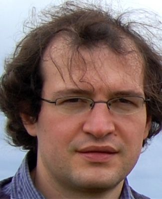
Laussy et al.: Superconductivity with excitons and polaritons: review and extension

                                 outstanding behavior of superconductivity, that is, conduction of electric charge by a macroscopic
                                 coherent wavefunction (akin to a Bose–Einstein condensate). It has taken some time to capture
                                 the fundamental and universal features of this phenomenon and set them apart from parti-
                                 cularities of certain cases only. The gap of excitations, responsible for zero resistivity, for instance,
                                 results from the long-range nature of the Coulomb interaction, but gapless superconductivity is
                                 also possible. One of the central, fundamental concepts of superconductivity is that of a coherent
                                 quantum state of charged bosons. Although superconductivity was discovered empirically, and its
                                 theoretical construction consisted in assembling a puzzle, it is now possible to envisage engineer-
                                 ing superconducting phases in other systems, based on this understanding of condensation of
                                 charged bosons. If superconducting phases can be identified in other systems, progresses will
                                 be quick for the understanding of cuprate superconductivity, which still eludes compelling
                                 theoretical explanation of its intrinsic mechanism.
                                      A system that is making rapid and impressive progress in terms of creating and controlling
                                 macroscopic quantum states is that of microcavity exciton-polaritons1 (see Ref. 2 for a review).
                                 These quasi-particles which combine properties of light (cavity photons) and matter (quantum
                                 well excitons) have been noted for their predisposition to accumulate in macroscopic number in a
                                 single or few quantum states.3,4 They have many advantages from a practical point of view, such
                                 as their 2D geometry, which allows straightforward manipulation by lasers impinging at an
                                 angle, and their short lifetime, which allows continuous monitoring of the system, reconstructing
                                 its internal dynamics also by angle-resolved spectroscopy.5 The pumping can be either coherent
                                 (driving states in parametric scattering configurations)6–10 or incoherent (with a constant flow of
                                 unrelated particles relaxing into the ground state).11–16 In nitride systems, the formidable claim
                                 has been made of room-temperature Bose–Einstein condensation.17,18 Recently, there has been
                                 great interest in propagation of polariton fluids19,20 and their superfluid properties,21 with reports
                                 of quantized vorticity22,23 and persistent currents.24
                                      These rising stars of macrosopic coherence have also been proposed to realize another much
                                 sought after quantum phase at high-temperature: superconductivity. Polariton condensates can-
                                 not conduct electric current themselves, being neutral particles. One of the proposed implemen-
                                 tations involves “ quatrons” (or quadrions) rather than polaritons.25 Quatrons are bound states of
                                 two electrons with a polariton. They remain bosons from spin-addition rules but carry an electric
                                 charge. A Bose condensate of quatrons would, through its superfluid propagation, exhibit super-
                                 conductivity. To date, however, the existence of the quatron, predicted theoretically,25 has not
                                 been found experimentally. Recently, we have approached the problem from another, and more
                                 conventional, angle, that of the Bardeen, Cooper, and Schrieffer (BCS) mechanism26 with an
                                 important new feature: replacement of phonons by Bose-condensed exciton-polaritons in the
                                 role of a binding agent between electrons. In the present paper, we generalize the model proposed
                                 in Ref. 26 to describe a wide range of hybrid Bose–Fermi semiconductor systems where a Bose–
                                 Einstein condensate of neutral quasi-particles (excitons or exciton-polaritons) coexists with a
                                 Fermi sea of electrons. We show that indeed such systems are promising for observation of
                                 (high-temperature) superconductivity. Moreover, as the superconducting gap and critical tem-
                                 perature are very sensitive to the concentration of bosons in the system and the latter may be
                                 controlled by direct optical excitation, light-induced superconductivity in semiconductor hetero-
                                 structures appears to be possible. In this work we closely follow the BCS approach, generalized
                                 and adapted to the case of superconductivity mediated by a Bose–Einstein condensate. Solving
                                 the gap equation in this case turns out to be a nontrivial problem, requiring careful analysis.

                                 1.1 BCS with a Bose–Einstein Condensate as a Binding Agent
                                 BCS is a pillar of superconductivity theory, which relies on three main tenets:
                                      1.     Instability of the Fermi sea,
                                      2.     Existence of an attractive interaction,
                                      3.     Condensation of charged bosons.
                                     These are the three insights that were mainly contributed by Cooper, Bardeen, and Schrieffer,
                                 respectively, and that they could assemble into the BCS theoretical edifice and exploit to repro-
                                 duce strikingly or predict successfully most of the superconductivity phenomenology.

                                 Journal of Nanophotonics                             064502-2                                  Vol. 6, 2012

Downloaded From: https://www.spiedigitallibrary.org/journals/Journal-of-Nanophotonics on 18 Sep 2021
Terms of Use: https://www.spiedigitallibrary.org/terms-of-use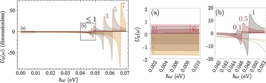
Laussy et al.: Superconductivity with excitons and polaritons: review and extension

                                      The first point follows from Cooper’s observation27 that an arbitrarily small attractive
                                 interaction between two electrons on top of the Fermi sea leads to a bound state (the Cooper
                                 pair), thanks to the truncation of the momentum space for states with wavevector k > kF (Fermi
                                 wavevector). This is a general result, which follows from the Bethe-Goldstone equation for the
                                 two-electron problem.
                                      The second point is the identification of an effective attraction between electrons that
                                 normally experience bare Coulomb repulsion. This attraction is attributed for conventional
                                 superconductors to an interaction through phonons, the Bardeen-Pines potential,28 that consists,
                                 vividly, of one electron wobbling the lattice at a first time, which affects another electron
                                 at a second time (and at a larger timescale, since the lattice dynamics is much slower than
                                 that of electrons).29 If the frequency of the lattice vibration is smaller than that of the propagating
                                 electron, the net effect results in an effective attraction [Leggett offers an insightful toy model
                                 of coupled oscillators to capture the essence of the interaction character (attractive or
                                 repulsive)].30
                                      The last point is the so-called BCS state, which is a coherent superposition of paired bound
                                 states and which brings the two-particle Cooper effect to a collective behavior of all electrons in
                                 the system.31
                                      With these three ingredients put together, the BCS theory is complete.32 For our purposes,
                                 points 1 and 3 will be regarded as fundamental and well-established features of (BCS type of)
                                 superconductivity. Point 2, which might appear a mere desiderata for point 1 to apply, leaves us
                                 room for identifying and designing new types of attractive potentials, optimizing the range of
                                 applicability and strength so as to obtain robust superconductivity (e.g., holding at high tem-
                                 peratures or high magnetic fields) or its manifestation in a new class of systems (in microcav-
                                 ities). Bardeen himself, with coworkers,33 investigated possibilities to engineer a more robust
                                 BCS state in a bilayer structure where excitons replace phonons as mediators of the interaction.
                                 The idea of substituting phonons by excitons was pioneered by Little34 and developed by
                                 Ginzburg,35 who coined the term and theorized the possibility of high-temperature supercon-
                                 ductivity, much before it came to fruition with cuprates.36 Cuprates, however, exploit another
                                 (still unknown) mechanism different to BCS.37
                                      In the following, we revisit the Ginzburg mechanism, based on BCS, with emphasis on max-
                                 imizing the strength of interaction between electrons, so as to maintain their binding, and therefore
                                 superconductivity, to higher temperatures. The text is organized as follows: in Sec. 2, we give a
                                 short overview of the BCS mechanism and the exciton (Ginzburg) mechanism, outlining the points
                                 of special interest in our case. In particular, we introduce the gap equation. In Sec. 3, we introduce
                                 our hybrid Bose–Fermi system configuration, its Hamiltonian and microscopic interactions, and
                                 the effective electron-electron Hamiltonian that results from a mean-field approximation for the
                                 condensate and the usual Frölich transformation. We obtain the shape of the effective electron-
                                 electron interaction U, that we find to be quite different in character to the Cooper (square well)
                                 potential. We also consider possible variations of our scheme, namely, a microcavity with a con-
                                 densate of exciton-polaritons and a condensate of indirect excitons in coupled quantum wells.38
                                 The system of coupled quantum wells explored by several groups39,40 might be easier to realize and
                                 study (it does not need a cavity) and presents some interesting differences as compared to the
                                 polariton system. On the other hand, polaritons condense at much higher temperatures.18 In
                                 Sec. 3.2, we study the gap equation for a Bose condensate-mediated effective interaction. Because
                                 the potential is not positive-definite, the problem is not well-posed numerically. We propose a
                                 simplified potential and an approximate solution of the gap equation, which we motivate by
                                 studying its validity on well-established approximations. We obtain the critical temperature in
                                 this case. In Sec. 4, we give our conclusions and perspective on this new application of excitons
                                 and polaritons and discuss how to measure the effect experimentally.

                                 2 BCS and Ginzburg Mechanisms
                                 Superconductivity is a fundamental property of solids. At low enough temperatures, most metals
                                 superconduct. As the mechanism is rooted in quantum mechanics, temperatures are expected to
                                 be very low and indeed this is the case for all metals. After considerable theoretical efforts

                                 Journal of Nanophotonics                              064502-3                                 Vol. 6, 2012

Downloaded From: https://www.spiedigitallibrary.org/journals/Journal-of-Nanophotonics on 18 Sep 2021
Terms of Use: https://www.spiedigitallibrary.org/terms-of-use
Laussy et al.: Superconductivity with excitons and polaritons: review and extension

                                 from various groups, a compelling theoretical model was assembled by Bardeen, Cooper, and
                                 Schrieffer, the so-called BCS theory.29 The model provides the critical temperature:

                                                                                    kB T C ¼ Θe−g ;
                                                                                                              1
                                                                                                                                         (1)

                                 where, in conventional superconductivity, Θ is the Debye energyℏωD, and g ¼ N ð0ÞV with
                                 N ð0Þ the density of electrons at the Fermi energy and V the electron-phonon coupling strength.
                                 The Debye energy is, in good approximation, the maximum energy that can be carried by a
                                 phonon. The mechanism therefore relies heavily on phonons, as was realized empirically before
                                 the advent of BCS (good conductors, for instance, are bad superconductors, since V is small; also
                                 through the isotope effect, which correlates critical temperature with mass of the crystal atoms,
                                 and thus with resonance frequency). The exponential form and the presence of N ð0Þ show
                                 that the effect is a collective one involving all electrons, which have formed a new phase of
                                 matter that cannot be approached perturbatively by the independent electron pictures (since
                                 f ðzÞ ¼ e−1∕z has no Taylor expansion around zero). Based on the theory, and accumulated
                                 experience, it was widely accepted that critical temperatures would not exceed a few tens
                                 of Kelvins, since the Debye energy, which can be quite large in some systems (hundreds
                                 of Kelvins), is exponentially reduced. In all conventional superconductors N ð0ÞV ≪ 1 (the
                                 so-called weak-coupling regime).
                                      Ginzburg made the obvious but daring assumption that to achieve higher critical
                                 temperatures—crucial for technical applications which can easily be understood to be momen-
                                 tous—it is enough to find a system where Θ and/or g are increased. Replacing phonons by
                                 excitons, for instance, Ginzburg found that values Θ∕kB ≈ 103 , 104 K as well as g ≈ 15, 13 are
                                 obtained, yielding temperatures of several hundred Kelvin.41 High critical temperatures have
                                 been later reported in cuprates36 and nowadays, temperatures as high as 125 K are obtained
                                 in systems such as Tl-Ba-Cu-oxide. Cuprate superconductivity does not appear to follow the
                                 BCS pattern.42 On the other hand, all attempts to date to realize the exciton mechanism or a
                                 variation of it have remained fruitless. This is this mechanism, rooted in BCS, which we consider
                                 in this text. Since it consists in substituting the phonons of conventional BCS—or the excitons of
                                 Ginzburg scheme—by a Bose–Einstein condensate (BEC) of excitons or exciton-polaritons,
                                 the starting point for its microscopic description starts with the same zero temperature
                                 gap equation:
                                                                                           X        Δ 0
                                                                              Δk ¼ −          U kk 0 k ;                                 (2)
                                                                                           k0
                                                                                                    2Ek 0

                                 where U kk 0 is the effective interaction between electrons with wavevectors k and k 0 and
                                 energy E. The gap Δ can be identified as the macroscopic wavefunction of a Cooper pair,
                                 which is also the order parameter for the superconducting phase. If it is nonzero, the system
                                 is in the superconducting state. A realistic microscopic treatment of U is very complicated.
                                 A simplified version is provided by the Jellium model, which is a toy model of a metal that
                                 gives predominance to electron-electron interactions, that is, in particular, the underlying crystal
                                 is approximated as a uniform (structureless) background (like a “jelly”) in which the interacting
                                 electron gas evolves under its own self-interactions and the overall charge cancellation of the
                                 background. A popular effective interaction is given by the Bardeen-Pines potential30 which is
                                 derived from the microscopic form of the electron-lattice interaction:

                                                                            κ0              ωph ðqÞ2
                                                          U BP ðω; qÞ ¼                1þ 2             ;                               (3a)
                                                                        1 þ q2 ∕q2TF     ω − ωph ðqÞ2

                                                                                          κ0
                                                                        ¼
                                                                                                   ω2
                                                                                                         ;                            (3b)
                                                                                   q2
                                                                             1þ   κ 23D
                                                                                               1 − ωi2

                                 with q the phonon wavevector. In Eq. (3a), qTF is the Thomas-Fermi screening parameter and ωph
                                 is the phonon dispersion. The first term between the brackets is bare Coulomb repulsion, and the

                                 Journal of Nanophotonics                                 064502-4                              Vol. 6, 2012

Downloaded From: https://www.spiedigitallibrary.org/journals/Journal-of-Nanophotonics on 18 Sep 2021
Terms of Use: https://www.spiedigitallibrary.org/terms-of-use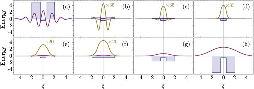
Laussy et al.: Superconductivity with excitons and polaritons: review and extension

                                 second term, which is frequency dependent, follows from the perturbative coupling to the lattice,
                                 tracing out the phonons.
                                     The physical meaning of Eq. (3a) is at the heart of the phonon-mediated mechanism. The
                                 interaction is ω dependent, which means, in Fourier transform, time dependent. This reflects the
                                 famous retardation effect in superconductivity. This effect is based on the strong difference
                                 between the electron Fermi velocity in metals and the sound velocity. Roughly speaking,
                                 a fast electron from the Fermi surface creates a slow phonon and goes away. After some
                                 time, another fast electron arrives and absorbs the slow phonon. The average distance between
                                 these two electrons remains of the order of 100 nm, the distance at which the screened Coulomb
                                 repulsion can be safely neglected. Due to the retardation effect, a weak phonon-mediated
                                 attraction of electrons wins over their Coulomb repulsion and provides formation of Cooper
                                 pairs at low enough temperatures.

                                 3 Interaction Hamiltonian
                                 A sketch of the structure we propose appears in Fig. 1(c). A QW is doped negatively (with
                                 density of electrons n) and is put in contact with another QW where excitons are formed
                                 and are stable. The first (lower) QW hosts the 2DEG which is to undergo superconductivity
                                 while the second (upper) QW hosts the condensate of excitons that is to mediate it. This structure
                                 can also be placed at the maximum of the optical field confined in a microcavity26 (formed by
                                 two Bragg mirrors facing each other). The latter configuration also has the advantage that two
                                 excitonic- QWs can sandwich the 2DEG-QW since in this case the condensate is delocalised
                                 in the entire structure thanks to the photon fraction of the polariton. This allows an increase by a
                                 factor of 2, or more if the multilayer structure is further repeated, of the densities achievable in
                                 this system. The drawback of microcavities is a short radiative lifetime of polaritons. In order to
                                 maintain the polariton condensate one needs to pump it resonantly by a high-intensity laser,
                                 which may lead to undesirable heating of the system. The alternative system which we consider
                                 is a condensate of long-living spatially indirect excitons in coupled QWs, separated by a thin
                                 but high barrier from a QW containing a two-dimensional electron gas (2DEG). This system is
                                 simpler to realize as it does not contain the optical cavity. The condensate of indirect excitons
                                 may be maintained by a low-intensity optical excitation. Moreover, indirect excitons in coupled
                                 QWs possess very significant dipole moments which strengthens their interaction with electrons
                                 from a 2DEG. However, Bose condensates of indirect excitons have been found only at tem-
                                 peratures below 1 K,38 while condensates of exciton-polaritons are now routinely produced at
                                 room-temperature.43 In the following, we compare the advantages of the two respective schemes.
                                 Most of the underlying model applies to both equally. We focus more particularly on the
                                 microcavity system since it is more general. The exciton system is recovered by decoupling
                                 the photons.

                                 Fig. 1 One of the possible designs to evidence exciton-polariton mediated superconductivity.
                                 (a) Polariton (thick blue solid line) and exciton (magenta dashed line) dispersions with schematic
                                 representation of scattering of the boson that mediates the interaction between electrons. Also
                                 shown in thin blue solid line is the renormalised dispersion E bog , essentially identical to E pol .
                                 (b) Corresponding scattering of two electrons on the surface of the Fermi sea, exchanging momen-
                                 tum q through scattering of a boson in panel (a). (c) detail of the sandwich structure, showing the
                                 doped well (below) containing free electrons and the well hosting the condensate (above) of exci-
                                 tons or of exciton-polaritons. This layer can be sandwiched in different ways.

                                 Journal of Nanophotonics                              064502-5                                 Vol. 6, 2012

Downloaded From: https://www.spiedigitallibrary.org/journals/Journal-of-Nanophotonics on 18 Sep 2021
Terms of Use: https://www.spiedigitallibrary.org/terms-of-use
Laussy et al.: Superconductivity with excitons and polaritons: review and extension

                                 Table 1 Parameters used in the numerical simulations. In square brackets, the value for the
                                 exciton case when the parameter differs from the polariton case, otherwise parameters have
                                 been taken the same for comparison.

                                 Parameter                                          Meaning                                                     Value

                                 ϵ                                 Permittivity                                                         7ϵ0 ≈ 6.2 As∕ðmVÞ
                                                                                                                                              0.22
                                 βe                                Electron reduced mass                                                   0.22þ1.25   ≈ 1.15
                                                                                                                                              1.25
                                 βh                                Hole reduced mass                                                       0.22þ1.25   ≈ 0.85

                                 L                                 Distance between wells                                                       5 nm

                                 κ                                 Coulomb screening length                                               ≈1.2 × 10⁹ m−1

                                 mx                                Exciton mass                                                 ð0.22 þ 1.25Þm e ≈ 1.3 × 10⁻³⁰ kg

                                 mc                                Photon mass                                                       10−5 m e ≈ 9.1 × 10−36 kg

                                 2g                                Rabi splitting                                                            45 meV [0]
                                                                                                                                                pffiffiffi
                                 X                                 Hopfield coefficient (exciton weight)                                      1∕ 2 [1]

                                 kF                                Fermi wavevector                                                         5 × 10⁸ m−1

                                 aB                                Exciton Bohr radius                                                     1.98 × 10⁻⁹ m

                                 Ry                                Exciton Rydberg                                                             32 meV

                                 d                                 Dipole moment                                                           4 nm [12 nm]

                                    In Fig. 1(a), the exciton (resp. polariton) dispersion is shown in dashed magenta (resp. solid
                                 blue). The difference between the bare polariton dispersion (thick blue) and the bogolon
                                 dispersion (thin blue) is very small over the range of exchanged momenta of interest (of the
                                 order of the Fermi wavevector). The condensate in both cases is at k ¼ 0. Scattered particles
                                 at any wavevector between −2k F and 2kF mediate electron-electron interactions on the
                                 Fermi sea, as sketched on Fig. 1(b). The model microscopic Hamiltonian is taken as:26
                                        X
                                   H¼      ½Epol ðkÞa†k ak þ Eel ðkÞσ †k σ k þ
                                           k
                                               X                                                                                                                     (4)
                                        þ               ½V C ðqÞσ †k1 þq σ †k2 −q σ k1 σ k2 ; þ X 2 V X ðqÞσ †k1 σ k1 þq a†k2 þq ak2 þ Ua†k1 a†k2 þq ak1 þq ak2 ;
                                            k1 ;k2 ;q

                                 with E pol ðkÞ and Eel ðkÞ the polariton and 2DEG dispersions for the in-plane wavevector k,
                                 respectively. In the exciton case (without the microcavity), it suffices to replace Epol with
                                 E ex in the above. V X is the electron-polariton interaction, U the polariton-polariton interaction
                                 and V C the electron-electron repulsion. We now consider these terms in turn. Parameters
                                 assumed are listed in Table 1.

                                 3.1 Electron-Electron Interaction
                                 In the original BCS mechanism, electron-electron repulsion is either neglected altogether or
                                 overcome by the attractive mechanism and not manifested outside of the attractive window.
                                 We take it into account here since it is a detrimental factor for binding and most of our concern
                                 for experimental realization is to optimize this value. The full form of the potential is given by the
                                 Yukawa potential:

                                                                                                     e2    1
                                                                                       V C ðqÞ ¼                ;                                                    (5)
                                                                                                    2ϵA jqj þ κ

                                 with screening constant κ. We get rid of the momentum dependence by averaging the potential
                                 V eff ðω; qÞ over the Fermi surface (FS), where:

                                 Journal of Nanophotonics                                       064502-6                                                 Vol. 6, 2012

Downloaded From: https://www.spiedigitallibrary.org/journals/Journal-of-Nanophotonics on 18 Sep 2021
Terms of Use: https://www.spiedigitallibrary.org/terms-of-use
Laussy et al.: Superconductivity with excitons and polaritons: review and extension

                                                          Fig. 2 Average over the Fermi surface, in 3D and 2D.

                                                                                                     q ¼ k1 − k2                                          (6)

                                 and k1;2 are the initial and final states of the electrons scattered with the exciton (polariton) from
                                 the condensate. The second electron scatters between states k10 and k20 such that k10 − k20 ¼ q.
                                 The characteristic energy EðqÞ is that of a bogolon (an elementary excitation of the condensate).
                                 In 3D, the FS where these electrons that scatter lie, is the surface of a sphere, while in 2D, it is a
                                 circle (we will speak of surface in both cases). The vector difference is therefore joining the two
                                 end-points on the surface. If the potential has spherical symmetry ½VðqÞ ¼ VðqÞ, the average of
                                 all two vectors on the FS reduces to that where q is pinned at one point of the surface (the south
                                 pole in Fig. 2) and runs overs the FS. This average, in the particular choice of Fig. 2, is the usual
                                 polar integration with k2 describing the surface as θ (and ϕ in 3D) are varied, with:

                                                                                 q2 ¼ 2k2F ð1 þ cos θÞ;                                                   (7)

                                 from Al Kashi’s theorem, so that the average potential V̄ eff reads, in 3D:
                                                                                Z       2π
                                                                                                Z    π
                                                              V̄ eff ðωÞ ¼                               V eff ðq; ωÞk2F sin θ dθdφ∕N ;                   (8)
                                                                                    0            0

                                 where N is the normalization, i.e., the same integral where V eff is replaced by unity. This gives,
                                 in 3D:
                                                                                Z                    qffiffiffiffiffiffiffiffiffiffiffiffiffiffiffiffiffiffiffiffiffiffiffiffiffiffiffiffiffiffi
                                                                            1           1
                                                            V̄ eff ðωÞ ¼                    V eff      2k 2F ð1 þ cos θÞ; ω d cos θ;                      (9)
                                                                            2    −1

                                                                                Z                     pffiffiffi
                                                                            1           4
                                                                        ¼                   V eff ðk F ϑ; ωÞdϑ;                                          (10)
                                                                            4       0

                                 where we integrate over ϑ ¼ 2ð1 þ cos θÞ since this is a natural variable in Eq. (7), and, in 2D:
                                                                                        Z                    qffiffiffiffiffiffiffiffiffiffiffiffiffiffiffiffiffiffiffiffiffiffiffiffiffiffiffiffiffiffi
                                                                                 1              2π
                                                             V̄ eff ðωÞ ¼                            V eff     2k 2F ð1 þ cos θÞ; ω dθ:                  (11)
                                                                                2π          0

                                     Our system is 2D, in which case, from Eqs. (5) and (11):
                                                                                                                 pffiffiffiffiffiffiffiffiffiffiffi
                                                                                                            2kF þ 4k 2F −κ2
                                                                2   Z                                    ln      p   ffiffiffiffiffiffiffiffiffiffiffi2
                                                            e     2π                dθ                 e    2kF − 4k2F −κ 2
                                                    V̄ C ¼           pffiffiffiffiffiffiffiffiffiffiffiffiffiffiffiffiffiffiffiffiffiffiffiffiffiffiffiffiffiffi ¼     pffiffiffiffiffiffiffiffiffiffiffiffiffiffiffiffi
                                                                                                                           ffi .                           (12)
                                                           4πϵA 0     2k 2F ð1 þ cos θÞ þ κ 2πϵA             4k 2F − κ2

                                    When κ > 2k F , both the numerator and the denominator become pure imaginary so their
                                 quotient remains real. When κ ¼ 2kF , V̄C ¼ e2 \ Φ2 \ εA \ κ. This is plotted in Fig. 3. Since
                                 we are trying to maximize attraction, that is, minimize repulsion, systems with small screening
                                 length and large wavevectors should be favored (but these parameters play critically on other
                                 aspects of the mechanism and the optimum is not compulsorily k F ∕κ ≫ 1).

                                 Journal of Nanophotonics                                                064502-7                                 Vol. 6, 2012

Downloaded From: https://www.spiedigitallibrary.org/journals/Journal-of-Nanophotonics on 18 Sep 2021
Terms of Use: https://www.spiedigitallibrary.org/terms-of-use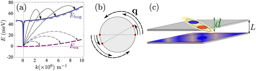
Laussy et al.: Superconductivity with excitons and polaritons: review and extension

                                 Fig. 3 Average electron-electron repulsion (in natural units) in the QW. This should be made as
                                 small as possible, which is obtained for higher Fermi wavevectors (for a given screening length).

                                 3.2 Electron-Exciton Interaction
                                 The electron-exciton or exciton-polariton interaction is one of the most important ingredients of
                                 the mechanism, as it ultimately determines the shape of the effective potential. In the micro-
                                 cavity, an electron (from the 2DEG) interacts with a polariton (from the condensate) through
                                 its excitonic component, so this is really the electron-exciton interaction that is to be computed,44
                                 weighted by the Hopfield coefficient (the excitonic fraction) X. Let us consider, therefore, the
                                 scattering of an electron in one of the parallel QW, separated by a distance L from the QW with
                                 excitons.45 The matrix element of the direct interaction between excitons and electrons reads:
                                                 Z
                                       V X ðqÞ ¼ ΨX ðQ; re ; rh ÞΨ ðk; r1 ÞVðr1 ; re ; rh ÞΨX ðQ; re ; rh ÞΨðk; r1 Þdr1 dre drh ; (13)

                                 where r1 , re , rh correspond to the 2D coordinates of the 2DEG electron, the exciton electron and
                                 the exciton hole respectively. The 2DEG electron is described by a plane wave while the electron/
                                 hole in the condensate are assumed to be in the 1s bound state with plane wave center-of-mass
                                 motion:
                                                                                            1
                                                                               Ψðq; r1 Þ ¼ pffiffiffi eikr1 ;                               (14a)
                                                                                             A
                                                                                   rffiffiffiffiffiffi
                                                                                      2 U e ðze ÞU h ðzh Þ iQ·RX −rX ∕aB
                                                             ΨX ðQ; re ; rh Þ ¼                          e     e        ;            (14b)
                                                                                    πA         aB

                                 where RX ¼ βe re þ βh rh , rX ¼ re − rh are in-plane coordinates of the center-of-mass of the
                                 exciton and relative coordinate of electron and hole in the exciton, U e ðze Þ and U h ðzh Þ are normal
                                 to the QW plane electron and hole envelope functions, respectively. We also consider the exis-
                                 tence of a dipole moment d for the exciton, which can be intrinsic to the structure, because of
                                 spatial separation of electrons and holes in coupled QWs, or (in the case of microcavities) be
                                 induced by an internal piezo-electric field, or result from an externally applied electric field. To
                                 account for all these possibilities, one can consider the layers of electrons and holes in the exci-
                                 ton shifted in the z-direction with respect to the position of the center-of-mass by a distance
                                 l ¼ d∕e ≪ L. The matrix element of the interaction is then computed to be:

                                                              e2 e−qL             1                      1
                                                 V dir ðqÞ ¼                                  −                                    (15a)
                                                             2ϵA q      ½1 þ ðβe qaB ∕2Þ2 3∕2 ½1 þ ðβh qaB ∕2Þ2 3∕2

                                                                  ed −qL             βe                    βh
                                                               þ     e                           þ                         ;          (15b)
                                                                 2ϵA       ½1 þ ðβe qaB ∕2Þ2 3∕2 ½1 þ ðβh qaB ∕2Þ2 3∕2

                                 Journal of Nanophotonics                              064502-8                                 Vol. 6, 2012

Downloaded From: https://www.spiedigitallibrary.org/journals/Journal-of-Nanophotonics on 18 Sep 2021
Terms of Use: https://www.spiedigitallibrary.org/terms-of-use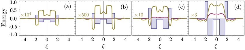
Laussy et al.: Superconductivity with excitons and polaritons: review and extension

                                 Fig. 4 Electron-exciton interaction in the geometry of Fig. 1, decomposed as the direct interaction
                                 (dashed magenta) and dipolar interaction (solid blue) when the exciton is induced with a dipole
                                 moment d . The latter is both much larger and maximum at zero exchanged momentum.

                                 where Eq. (15a) is the direct electron-exciton interaction that exists even in the absence of a
                                 dipole moment of the exciton, and Eq. (15b) is the dipolar interaction. The direct interaction
                                 vanishes at small exchanged momenta, while the dipolar-induced one assumes its maximum
                                 value here of 2d∕ð2ϵ0 ϵAÞ. Overall, the dipolar interaction is naturally much larger than the direct
                                 one, since the exciton is electrically neutral.* These facts are summarized in Fig. 4.

                                 3.3 Polariton-Polariton Interaction
                                 We treat the polariton-polariton interaction within the s-wave scattering approximation with
                                 strength U ¼ 6a2B Ry X 4 ∕A (where aB is the exciton Bohr radius, Ry the exciton binding energy
                                 and A the normalization area. X is the exciton Hopfield coeffcient, the square of which quantifies
                                 the exciton fraction in the exciton-polariton condensate).46 For interaction between bare exci-
                                 tons, X ¼ 1. Exciton-exciton (polariton-polariton) interactions are repulsive, in general. They
                                 result in linearization of the elementary excitation spectra, the Bogoliubov dispersion, but its
                                 role is not crucial to the mechanism of superconductivity we discuss, since at the wavevectors
                                 of interest, the changes brought by this term are very small compared to the kinetic energy of
                                 noninteracting excitons (exciton-polaritons).

                                 3.4 Effective Interaction
                                 We now proceed to bring our microscopic model toward a form suited to study Cooper-pairing
                                 and superconductivity, that is, we apply the canonical Fröhlich transformation that will result in
                                 an effective BCS Hamiltonian. Just as in the case of phonons, we start by getting rid of polar-
                                 itons. We assume a condensate is formed with mean population N 0 . We do not consider which
                                 mechanism, coherent or incoherent, is responsible for creating and maintaining this state. We do
                                 assume, however, it is coherent and with a definite phase, so that         weffi can apply the mean-field
                                                                                                       pffiffiffiffiffiffiffiffi
                                 approximation a†k1 þq ak1 ≈ ha†k1 þq iak1 þ a†k1 þq hak1 i and hak i ≈ N 0 Aδk;0 with N 0 the density of
                                 polaritons in the condensate. This allows us to obtain the following expression for the Hamil-
                                 tonian, after diagonalizing the polariton part by means of a Bogoliubov transformation (that
                                 leaves the free propagation of electrons and their direct interaction, H C , invariant):
                                                 X                     X                          X
                                           H¼       E el ðkÞσ †k σ k þ   E bog ðkÞb†k bk þ H C þ       MðqÞσ †k σ kþq ðb†−q þ bq Þ;  (16)
                                                        k                          k                                   k;q

                                 where Ebog ðkÞ describes the dispersion of the elementary excitations (bogolons) of the interact-
                                 ing Bose gas, which is very close to a parabolic exciton dispersion at large k:

                                 *Note at this point that there is an error in Ref. 26 where only the direct exciton interaction has been taken into account with an incorrect
                                 power in the parenthesis, which led to an expression similar to the dipolar interaction. The direct interaction by itself turns out to be too
                                 small to evidence superconductivity with the parameters chosen in Ref. 26, therefore a dipole moment should be induced in this case, say
                                 by applying an external electric field, to restore the effect.

                                 Journal of Nanophotonics                                        064502-9                                                    Vol. 6, 2012

Downloaded From: https://www.spiedigitallibrary.org/journals/Journal-of-Nanophotonics on 18 Sep 2021
Terms of Use: https://www.spiedigitallibrary.org/terms-of-use
Laussy et al.: Superconductivity with excitons and polaritons: review and extension
qffiffiffiffiffiffiffiffiffiffiffiffiffiffiffiffiffiffiffiffiffiffiffiffiffiffiffiffiffiffiffiffiffiffiffiffiffiffiffiffiffiffiffiffiffiffiffiffiffiffiffiffi
E bog ðkÞ ¼ Ẽpol ðkÞðẼ pol ðkÞ þ 2UN 0 AÞ; (17)
where Ẽ pol ðkÞ ≡ E pol ðkÞ − E pol ð0Þ and with the renormalized bogolon-electron interaction
strength:
sffiffiffiffiffiffiffiffiffiffiffiffiffiffiffiffiffiffiffiffiffiffiffiffiffiffiffiffiffiffiffiffiffiffiffiffiffiffiffiffiffiffiffiffiffiffiffiffiffiffiffiffiffiffiffi
pffiffiffiffiffiffiffiffiffi Ebog ðqÞ − Ẽ pol ðqÞ
MðqÞ ¼ N 0 AX 2 V X ðqÞ : (18)
2UN 0 A − E bog ðqÞ þ Ẽ pol ðqÞ
The last term of Eq. (16) coincides with the Fröhlich electron-phonon interaction Hamilto-
nian, which allows us to write an effective Hamiltonian for the bogolon-mediated electron-
electron
P interaction. This results in an effective interaction between electrons, of the type
† †
k1 ;k2 ;q V eff ðq; ωÞσ k1 σ k1 þq σ k2 þq σ k2 . The effective interaction strength reads V eff ðq; ωÞ ¼
V C ðqÞ þ V A ðq; ωÞ, with:
2MðqÞ2 Ebog ðqÞ
V A ðq; ωÞ ¼ : (19)
ðℏωÞ2 − Ebog ðqÞ2
Equation (19) recovers the boson-mediated interaction potential obtained for a Bose–Fermi
mixture of cold atomic gases,47 in the limit of vanishing exchanged wavevectors. It describes the
BEC induced attraction between electrons. Remarkably, it increases linearly with the condensate
density N 0. This represents an important advantage of this mechanism of superconductivity with
respect to the earlier proposals of exciton-mediated superconductivity,33,34,48 as the strength of
Cooper coupling can be directly controlled by optical pumping of the exciton-polariton conden-
sate. The attractive potential is displayed for various exchanged energies in Fig. 5, as a function
of θ, defining the exchanged momentum expressed directly through the angle θ defined in the
Fermi circle (cf. Fig. 2). As commented earlier, the negative part corresponds to attraction, and
the potential alternates between repulsive and attractive character, obtained at different
exchanged momenta. We do not want to keep track of such complicated wavevector dependence,
and therefore will average the interaction over the Fermi sea. A notable
pffiffiffiffiffiffiffiffiffiffiffiffiffiffiffiffiffiffiffiffiffiffiffiffiffiffiffiffiffi
ffi feature is, for most
values of ω, the presence of a pole θ0 , where E bog ½ 2k2F ð1 þ cos θ0 Þ ¼ ℏω. As is seen in
the figure, θ0 separates the attractive part from the repulsive part. The average will bring the
additional convenience of canceling such divergencies. We note as well that the spectrum of
excitations of the exciton-BEC may be changed in the presence of the electron gas, so that
their eventual dispersion may be different to E bog .49 This has no effect on the Cooper-pairing
of electrons which we discuss here.
We therefore wish to perform the average
Z 2π
U 0 ðωÞ ¼ V A ðq; ωÞdθ; (20)
0
Fig. 5 Effective electron-electron interaction as a function of θ, defining the exchanged momen-
pffiffiffi pffiffiffiffiffiffiffiffiffiffiffiffiffiffiffiffiffiffiffiffi
tum q ¼ 2k F 1 þ cos θ on the Fermi sea at energies ℏω ¼ 40, 50, and 60 meV, respectively.
The potential is symmetric around π. In the first case, the whole dependency (over ½0; 2π) is
shown, with a first zoom in the inset showing two poles and another the attractive region that
is of small amplitude but extends over a large range. With increasing energies, the poles recede
towards smaller values of θ with a dominating effect of the repulsive (positive) energy. In the
central panel, in dashed magenta, the regularized potential is superimposed.
Journal of Nanophotonics 064502-10 Vol. 6, 2012
Downloaded From: https://www.spiedigitallibrary.org/journals/Journal-of-Nanophotonics on 18 Sep 2021
Terms of Use: https://www.spiedigitallibrary.org/terms-of-useLaussy et al.: Superconductivity with excitons and polaritons: review and extension
pffiffiffiffiffiffiffiffiffiffiffiffiffiffiffiffiffiffiffiffiffiffiffiffiffiffiffiffiffiffi
where q ¼ 2k 2F ð1 þ cos θÞ, as seen previously. Since V A is symmetric around π we perform
the integral ∫ π0 only. The integral would be easily computed numerically if there were no pole.
There are dedicated numerical methods to compute principal values numerically,50,51 but in our
case, since the pole is first order, it is enough to isolate it analytically by defining
f ðθÞ ¼ ðθ − θ0 ÞV A ½qðθÞ; ω; (21)
so that
Z 2π f ðθÞ − f ðθ0 Þ 2π − θ0
U0 ¼ dθ þ f ðθ0 Þ ln ; (22)
0 θ − θ0 θ0
where f ðθ0 Þ ¼ limθ→θ0 f ðθÞ and the first integral is regular (it is shown in Fig. 5 in dashed magenta).
The integration (average) is then straightforward and produces the results shown in Fig. 6.
If we take instead of E pol a quadratic dispersion for the excitation
ℏ2 k 2
E x ðkÞ ¼ (23)
2mx
and assume all-excitonic interactions, X ¼ 1, we can consider the same effect in the absence of a
microcavity, relying on a purely excitonic (rather than polaritonic) BEC. In this case, the same
procedure as detailed above leads to an effective potential as shown in Fig. 7. We kept all para-
meters the same for comparison except for the dipole moment, which we have taken three times
as large (d ¼ 12 nm). This corresponds to the spatial separation of electrons and holes in the
Fig. 6 Exchanged-momentum averaged interaction U 0 ðωÞ between electrons of the 2DEG, as N 0
is increased. It is dimensionless and is attractive (resp. repulsive) when negative (resp. positive).
Densities N 0 are shown in units of 1012 ∕cm2 . In insets (a) and (b), a zoom of the regions delineated
on the left panel, firstly in the small energies (long time) range, where the attraction is seen to be
repulsive for smaller densities, because of the Coulomb repulsion (shown in red), and secondly for
the densities ≈1012 ∕cm2 in the area where the character of the interaction changes abruptly from
attractive to repulsive (higher densities are shown in dotted lines).
Fig. 7 Same as Fig. 6 (also in units of 1012 ∕cm2 ) but for the case of an exciton condensate. A
larger dipole moment d has also been assumed. The potential is different in character, much clo-
ser to Cooper’s potential with larger attraction at longer times.
Journal of Nanophotonics 064502-11 Vol. 6, 2012
Downloaded From: https://www.spiedigitallibrary.org/journals/Journal-of-Nanophotonics on 18 Sep 2021
Terms of Use: https://www.spiedigitallibrary.org/terms-of-useLaussy et al.: Superconductivity with excitons and polaritons: review and extension
system of indirect excitons studied by Butov et al.38 The potential we obtain in the exciton case is
very different in character from the polariton case, and is more closely related to the Cooper
(conventional) shape of a square well, or the Bogoliubov potential including repulsive elbows.
From these potentials, one can proceed to solve the gap equation.
4 Gap Equation
4.1 Cooper Potential
The BCS gap equation (2) is easier to tackle as a continuous equation:
Z ∞
U 0 ðξ − ξ 0 ÞΔðξ 0 ; TÞ tanhðE∕2k B TÞ 0
Δðξ; TÞ ¼ − dξ ; (24)
−∞ 2E
pffiffiffiffiffiffiffiffiffiffiffiffiffiffiffiffiffiffiffiffiffiffiffiffiffiffiffiffiffiffi
E ¼ Δðξ 0 ; TÞ2 þ ξ 02 where we have also introduced a finite temperature T from the Fermi-
Dirac distribution of elementary excitations.52 With the BCS approximation of a step potential,
the gap equation at zero temperature simplifies to Δðξ; TÞ ¼ −U 0 ∫ ξþℏω 0 0
ξ−ℏωD Δðξ ; TÞ∕2Edξ . If
D
Δ ≫ ℏωD , the ξ dependence in the integral boundaries can be neglected (or, coming back to
Eq. (2), one sees that in the initial gap equation, Δk is exactly constant if U kk 0 ¼ U 0 and is
zero otherwise). Thus, we can assume in this case the gap to be of the form:
Δð0Þ if jξj ≤ ℏωD ;
ΔðξÞ ¼ (25)
0 otherwise:
In this case, simplifying Δð0Þ on both side of Eq. (24), we obtain:
Δð0Þ ¼ ℏωD ∕ sinhð1∕U 0 Þ: (26)
Equation (26) is better known as its approximation when U 0 ≪ 1, in which case it takes the
form of the famous BCS gap expression,
Δð0Þ ≈ 2ℏωD expð−1∕U 0 Þ (27)
Solving exactly the gap equation calls for some numerical method. Equation (24) is a non-
linear integral equation, of the type studied by Hammerstein, i.e.,
Z
Δðξ; TÞ ¼ Kðξ; ξ 0 Þf ½ξ 0 ; Δðξ 0 Þdξ 0 (28)
pffiffiffiffiffiffiffiffiffiffiffiffiffiffi pffiffiffiffiffiffiffiffiffiffiffiffiffiffi
where in our case Kðx; yÞ ¼ −U 0 ðx − yÞ∕2 and f ½y; z ¼ z tanhð y2 þ z2 Þ∕ y2 þ z2 . There are
strong conditions of existence of non-trivial (nonzero) solutions when U 0 ≤ 0;53,54 however, the
case when the kernel K is not positive-definite, that is, in presence of repulsion,† has been much
less studied mathematically.55 Cooper’s potential, being always negative, falls in the category of
potentials which admit a unique non-trivial solution, with a stable numerical technique to obtain
it, namely, since the mapping is contractive, by iterations of the gap equation: an initial (nonzero)
function Δ0 is used to compute the rhs of Eq. (24), providing Δ1 which is injected back until
the function converges. The gap computed in this way for a given Cooper potential is shown in
Fig. 8(a). As one can see, the BCS approximation [Eq. (26)] remains a rather coarse approx-
imation, since the gap turns out in this case to be bell-shaped rather than being a step function.
Surprisingly, Δð0Þ is however in much closer agreement with its approximation [Eq. (28)], as
shown on Fig. 8(b) and 8(c) in the weak and strong coupling regime, respectively. There are
small quantitative deviations in (b) between the numerical points and the formula when
using the exact parameters of the potential. By fitting the numerical results, a perfect agreement
can be found for slight variations of ℏωD and U 0 . The BCS approximation therefore turns out to
be an exceedingly good one as compared to an exact solution of the gap equation. For the
†
as well as attraction, since the case of only repulsion admits only Δ ¼ 0 as a solution.
Journal of Nanophotonics 064502-12 Vol. 6, 2012
Downloaded From: https://www.spiedigitallibrary.org/journals/Journal-of-Nanophotonics on 18 Sep 2021
Terms of Use: https://www.spiedigitallibrary.org/terms-of-useLaussy et al.: Superconductivity with excitons and polaritons: review and extension
Fig. 8 Numerical solution to the gap equation with the BCS square well potential (a). The gap ΔðξÞ
is not step-wise as approximated in the BCS model, but its value at zero exchanged energy, Δð0Þ,
is in close agreement with the analytical expressions, as seen in (b) and (c): Δð0Þ as obtained from
numerically solving the gap equation (dashed blue) and from Eq. (26) (solid magenta), (b) in the
weak-coupling limit when U 0 ≪ 1, with small deviations as coupling is increased, and (c) in the
strong-coupling where the agreement becomes perfect again. Note that Δ increases linearly with
the coupling strength out of the weak-coupling limit.
procedure to make sense, similar results should be obtained for a smoothed well that approx-
imates the BCS square well.41 We will not address this point here, but go directly to the case
where the potential is not always attractive.
4.2 Bogoliubov Potential
The potential is not always attractive when, for instance, some overall repulsion, such as direct
Coulomb interaction, is superimposed on the attractive Cooper potential, as shown on Fig. 9. The
Coulomb interaction is time independent and should therefore extend to all ω but here also a
cutoff ωC is introduced to avoid divergencies. This results in an attractive, Cooper-like potential,
flanked by two repulsive windows. Such a potential is known as the Bogoliubov potential.56,57
This approximation has been used to show extremely counterintuitive behavior of the gap
equation and justify a-posteriori another heavily criticized approximation of BCS, neglecting
Coulomb repulsion: the BCS mechanism indeed assumes only attraction between electrons,
which can be dimmed by Coulomb repulsion, but which never explicitly appears as such
(like in the Bogoliubov scenario). The great result of Cooper was that binding occurs at
arbitrarily small attraction. An important result of the Bogoliubov potential is to show that
the detrimental effects of Coulomb repulsion are greatly reduced in the gap.57
We now present a linearization of the gap equation that allows one to obtain an approximate
solution for the critical temperature.56 By assuming the gap equation to be a two-step valued
function Δ ¼ ðΔ1 ; Δ2 ÞT , the gap equation becomes ðI − 1ÞΔ ¼ 0 with
−U 0 I 1 V C I 2
I¼− ; (29)
V CI 1 V CI 2
where
Z
ℏωDtanh ½ξ∕ð2kB T C Þ 1.13ℏωD
I1 ¼ pffiffiffiffiffiffiffiffiffiffiffiffiffiffiffiffi dξ ≈ ln ; (30a)
−ℏωD ξ 2
þ Δ 2
1
kB T C
Fig. 9 Adding an overall repulsive Coulomb repulsion V C (red, left) until a cutoff ωC to the BCS
potential V 0 (green, left) results in the Bogoliubov step-wise potential (right). We take the conven-
tion V 0 , V C , U 0 positive in the above representation and U 0 ¼ V 0 − V C , so that, e.g., V C < 0
means attractive contribution of the “Coulomb repulsion.”
Journal of Nanophotonics 064502-13 Vol. 6, 2012
Downloaded From: https://www.spiedigitallibrary.org/journals/Journal-of-Nanophotonics on 18 Sep 2021
Terms of Use: https://www.spiedigitallibrary.org/terms-of-useLaussy et al.: Superconductivity with excitons and polaritons: review and extension
Z
ℏωC tanh ½ξ∕ð2k B T C Þ ω
I2 ¼ pffiffiffiffiffiffiffiffiffiffiffiffiffiffiffiffi dξ ≈ ln C ; (30b)
ℏωD ξ þ Δ2
2 2 ω D
appear invariably in the columns of I. In Eq. (30a), the BCS approximation has been applied
while in Eq. (30b), the fact that jξj ≫ 0 has been used to neglect Δ in the denominator and the
temperature in the numerator. The parametrization of the matrix in terms of the potential depends
on the particular configuration (for example the relative widths of the various layers of the struc-
ture). Here we have adopted the original parametrization of Bogoliubov, which assumes narrow
repulsive elbows surrounding a large attractive central region. Solving the linear equation for I 1
and then for the critical temperature, we find:
1
k B T C ≈ 1.13ℏωD exp − : (31)
V 0 − 1þIV C2 V C
In this form, one can see how Coulomb repulsion indeed introduces a small correction to the
original BCS formula. The expression also seems to indicate that U 0 could be repulsive
(V 0 − V C < 0) and still lead to a gap as long as the denominator in Eq. (31) remains positive.
In the following, we compare these predictions with numerical solutions of the gap equation,
keeping in mind that the iterative procedure is not assured, mathematically, to converge. We have
observed that indeed, it sometimes encounters problems and exhibits strong instabilities, with
bifurcations of solutions, for example.
In Fig. 10, we show the evolution of the gap function as V C is increased, from zero (BCS) to a
point where the overall potential is essentially repulsive. With onset of the repulsion, the gap
acquires two negative sides and becomes a highly distorted function for large V C . Note that the
approximation of constant gap over the various regions is at least as good as for the case of BCS.
In Fig. 11, we now show the case where U 0 ¼ V 0 − V C is held constant as the strength of the
repulsion is varied independently. In foresight of what is to come later, we also allow the elbows
to be negative, that is, to contribute an additional attraction to the conventional mechanism (for
now we do not consider physical justification of this). Another unexpected result is obtained:
the repulsive potential is in this case favoring a larger gap, as can be seen by comparing (a),
where the gap function is highly oscillatory, to (d) where it recovers the BCS bell-shape. In (h),
the distorted but overall attractive potential still results in a BCS type gap, but wider and larger.
Note how the repulsion, by “squeezing” the gap, allows it to achieve much higher values than for
the case of smaller or no repulsion.
These unexpected results are confirmed phenomenologically by the Bogoliubov approxima-
tion Eq. (31), which reproduces qualitatively the trend of the gap Δð0Þ as shown in Fig. 12. Here
we should emphasize that the two quantities are not meant to be compared quantitatively, since
one, Δð0Þ (computed numerically) is the gap at zero temperature while the other, kB T C is the
temperature at which the gap vanishes. There is a monotonous relationship between the two, that
is, increasing Δð0Þ implies increasing T C , so one can appreciate the consistency of the results by
observing similar trends. The obstacle to conducting an extensive numerical comparison is that it
is an intensive task numerically to compute T C , since this requires solution of the gap equation
for various temperatures until the curve ΔðTÞ is obtained and its intersect with zero is found.
Fig. 10 Gap (thick magenta and, magnified, thick khaki) of the Bogoliubov potential (filled blue)
solved numerically for the parameters: ℏωD ¼ 1, ℏωC ¼ 2, V 0 ¼ 1 and V C taking values from (a) to
(d) of: 0 (BCS), 0.1, 0.3 and 0.495. Coulomb repulsion results in a dip in the gap function that, for
increasing values, results in oscillations in the gap function. Paradoxically, even when it is large
and dominating attraction, repulsion does not prevent a gap, as seen in (d).
Journal of Nanophotonics 064502-14 Vol. 6, 2012
Downloaded From: https://www.spiedigitallibrary.org/journals/Journal-of-Nanophotonics on 18 Sep 2021
Terms of Use: https://www.spiedigitallibrary.org/terms-of-useLaussy et al.: Superconductivity with excitons and polaritons: review and extension
Fig. 11 Gap (thick magenta and, magnified, thick khaki) of the Bogoliubov potential (filled blue)
solved numerically for the following parameters: ℏωD ¼ 0.5, ℏωC ¼ 2, V 0 − V C ¼ 0.5 (fixed) and
V C (the height of the elbow) taking values from (a) to (h) of: −5, −0.5, −0.1, 0 (BCS), 0.3, 0.5
(BCS), 1.5 and 5. The repulsive nature of the elbows change the character of the gap from
bell-shaped to an oscillating function. The oscillating gap in the presence of strong repulsion
allows, paradoxically, high values of the gap at zero-exchanged energy.
Fig. 12 Δð0Þ for the case of Figs. 10(a) and 11(c), for their respective parameters, and (b), with
ℏωD ¼ :5, V 0 ¼ 1, ωC changing as indicated and V C changing such that the area of the repulsive
elbow is conserved.
A critical slowing down phenomenon makes the iterative process slower as the critical tempera-
ture is approached. In addition, numerical instabilities are stronger at nonzero T. Therefore,
although it is relatively straightforward to compute Δð0Þ numerically, it is not convenient to
use this method to obtain T C . On the other hand, the Bogoliubov approximation gives a fair
estimate of T C , but is not able to provide the gap at zero temperature, since at the core of
its method, there is an assumption of vanishing Δ. Therefore, we have two complementary
methods, each suited to provide a relevant aspect of the problem. We note that the gap at
zero temperature is an important quantity which can be measured independently from T C by
Andreev reflection in conductivity experiments.
4.3 Polariton Potential
In the case of the polariton problem, we have seen that, even when neglecting Coulomb repulsion
(as in the original BCS formulation), the potential UðωÞ departs strongly from the Cooper poten-
tial and features two large attractive regions far from small energies, immediately followed by
two strong repulsive windows. We extend the Bogoliubov method to a three-step approximation
of this potential, such as displayed in Fig. 13, with, in reference to previous potentials, notations
ωD , ωC and ωB for the boundaries of the central, shallow attractive region, narrow, deep attractive
region and repulsive region, respectively. This is a notation only and is not mean to be under-
stood as referring to Debye, Coulomb, or Bogoliubov in any strict sense. Following the same
premises, we approximate the gap equation by a three-step valued function Δ ¼ ðΔ1 ; Δ2 ; Δ3 ÞT .
This approximation turns out to be an exceedingly good one in certain cases, such as the one
displayed in Fig. 13, where the gap itself is also a three-steps function in good approximation.
Here there is even more room to choose a parametrization of the I matrix. We now give general
guidelines on how to build this matrix. The simplest method is to fix ξ on the lhs of Eq. (25) at the
Journal of Nanophotonics 064502-15 Vol. 6, 2012
Downloaded From: https://www.spiedigitallibrary.org/journals/Journal-of-Nanophotonics on 18 Sep 2021
Terms of Use: https://www.spiedigitallibrary.org/terms-of-useYou can also read