Optimized Atomic Partial Charges and Radii Defined by Radical Voronoi Tessellation of Bulk Phase Simulations - MDPI
←
→
Page content transcription
If your browser does not render page correctly, please read the page content below
molecules
Article
Optimized Atomic Partial Charges and Radii Defined by
Radical Voronoi Tessellation of Bulk Phase Simulations
Martin Brehm *               and Martin Thomas

                                          Institut für Chemie, Martin-Luther-Universität Halle–Wittenberg, von-Danckelmann-Platz 4,
                                          D-06120 Halle (Saale), Germany
                                          * Correspondence: Martin_Brehm@gmx.de

                                          Abstract: We present a novel method for the computation of well-defined optimized atomic partial
                                          charges and radii from the total electron density. Our method is based on a two-step radical Voronoi
                                          tessellation of the (possibly periodic) system and subsequent integration of the total electron density
                                          within each Voronoi cell. First, the total electron density is partitioned into the contributions of each
                                          molecule, and subsequently the electron density within each molecule is assigned to the individual
                                          atoms using a second set of atomic radii for the radical Voronoi tessellation. The radii are optimized
                                          on-the-fly to minimize the fluctuation (variance) of molecular and atomic charges. Therefore, our
                                          method is completely free of empirical parameters. As a by-product, two sets of optimized atomic
                                          radii are produced in each run, which take into account many specific properties of the system
                                          investigated. The application of an on-the-fly interpolation scheme reduces discretization noise in the
                                          Voronoi integration. The approach is particularly well suited for the calculation of partial charges in
                                          periodic bulk phase systems. We apply the method to five exemplary liquid phase simulations and
                                show how the optimized charges can help to understand the interactions in the systems. Well-known

                                          effects such as reduced ion charges below unity in ionic liquid systems are correctly predicted without
Citation: Brehm, M.; Thomas, M.           any tuning, empiricism, or rescaling. We show that the basis set dependence of our method is very
Optimized Atomic Partial Charges          small. Only the total electron density is evaluated, and thus, the approach can be combined with
and Radii Defined by Radical Voronoi
                                          any electronic structure method that provides volumetric total electron densities—it is not limited
Tessellation of Bulk Phase
                                          to Hartree–Fock or density functional theory (DFT). We have implemented the method into our
Simulations. Molecules 2021, 26, 1875.
                                          open-source software tool TRAVIS.
https://doi.org/10.3390/
molecules26071875
                                          Keywords: atomic partial charges; Voronoi tessellation; molecular dynamics; electron structure
Academic Editor: Stacey Wetmore
                                          theory; numerical integration; non-linear optimization; bulk phase; liquid phase; hydrogen bond

Received: 28 February 2021
Accepted: 24 March 2021
Published: 26 March 2021                  1. Introduction
                                                The determination of atomic partial charges in chemical systems is important for many
Publisher’s Note: MDPI stays neutral      fields of computational chemistry, e.g., to parametrize force fields for classical molecular
with regard to jurisdictional claims in   dynamics simulations, which are known to depend sensitively on the atomic charges [1–3],
published maps and institutional affil-   or even for estimating the electronic correlation energy [4,5]. As partial charges are not
iations.                                  quantum mechanical observables, no canonical way exists to derive them, and a plethora of
                                          methods to define these partial charges has been proposed. The most popular techniques
                                          can be classified according to a few general ideas. The first approach relies on a partitioning
                                          of the molecular wave function expressed in terms of basis functions. This class includes,
Copyright: © 2021 by the authors.         e.g., Mulliken population analysis [6], Löwdin population analysis [7,8], and natural
Licensee MDPI, Basel, Switzerland.        population analysis (NPA) [9]. Recently, similar tools have become available for plane-
This article is an open access article    wave calculations of solid-state materials [10,11], based on analytical projections of the
distributed under the terms and           PAW wave function [12]. Another group of methods is based on the molecular electrostatic
conditions of the Creative Commons        potential: a certain set of points is chosen and the partial charges are fitted to reproduce
Attribution (CC BY) license (https://
                                          the electrostatic potential given by the molecular wave function at these points [13–15].
creativecommons.org/licenses/by/
                                          The commonly applied CHELPG charges [16,17] and RESP charges [18] are, e.g., obtained
4.0/).

Molecules 2021, 26, 1875. https://doi.org/10.3390/molecules26071875                                      https://www.mdpi.com/journal/molecules
Molecules 2021, 26, 1875                                                                                            2 of 22

                           in this way. The dynamically generated RESP charges [19–21] follow a very similar idea.
                           Further techniques are closely related to the multipole moments of the molecular charge
                           distribution, e.g., generalized atomic polar tensor charges [22], density derived atomic
                           point charges (DDAPC, Blöchl charges) [23], and local multipole-derived charges [24].
                                 Atomic partial charges obtained by spatially partitioning the electron density have
                           also been of interest for a long time. There exist two general concepts that use either diffuse
                           weighting functions on the atoms, or distinct boundaries between them. In the former
                           concept introduced by Hirshfeld [25], the weighting functions are derived from a pro-
                           molecular density that consists of the spherically averaged ground-state atomic densities.
                           The definition of the weighting functions was modified later on to extend the applicability
                           of this approach to a broader range of systems [26–29]. Stewart atoms are also diffuse and
                           they possess a spherical shape that is fitted to reproduce the molecular electron density
                           as close as possible [30,31]. Concerning the second concept, distinct boundaries between
                           the atoms can be obtained by a topological analysis of the electron density as in Bader’s
                           theory of atoms in molecules [32,33]. Another possibility are purely geometric criteria such
                           as the Voronoi tessellation [34–36], where a simple plane is placed midway between two
                           atoms [37]. This idea was extended later on to account for different atom sizes by shifting
                           the boundary planes [38–41], for example in Richards’ “method B” [42] which found some
                           applications [40]. A combination of both general concepts discussed above are Voronoi
                           deformation density charges, where the deformation density of Hirshfeld’s approach is
                           integrated in Voronoi cells around the atoms [43].
                                 In this article, we present a new method to calculate atomic partial charges by parti-
                           tioning the electron density. We follow the previous idea of using the distinct boundaries
                           of a Voronoi tessellation, but we employ a generalization in terms of the radical Voronoi
                           tessellation (also known as “power diagram” in the two-dimensional case) [44]. In this
                           technique, a radius is assigned to each atom, allowing to model the sizes of the atoms
                           in a chemically reasonable sense. Such radii have also been used in reference [40], but
                           instead of the ratio of the radii, the difference of the squared radii determines the position
                           of the cell face between two atoms here. Thus, in contrast to the aforementioned “method
                           B” [40,42] and similar approaches, the radical Voronoi tessellation does not suffer from
                           the “vertex error” [42,44], i.e., it does not contain holes. When integrating electron density,
                           this is important to keep the total charge of the system constant. As another advantage,
                           the Voronoi sites around which the cells are constructed can be kept on the atoms and do
                           not have to be shifted (as it was done in reference [39]) to obtain a chemically reasonable
                           partitioning. To the best of our knowledge, the radical Voronoi tessellation has not been
                           used for the computation of atomic partial charges before.
                                 The crucial parameters in the radical Voronoi tessellation are the radii assigned to the
                           atoms. We have recently shown [45] that van der Waals radii [46–48] yield a reasonable
                           separation of molecules in the bulk phase, and that the resulting molecular electromagnetic
                           moments can readily be used to calculate vibrational spectra of bulk phase systems from ab
                           initio molecular dynamics (AIMD) simulations, including infrared [45,49,50], Raman [45],
                           vibrational circular dichroism (VCD) [51], Raman optical activity (ROA) [52], and resonance
                           Raman [53] spectra. Since van der Waals radii have been fitted to reproduce intermolecular
                           distances, it can be expected that they lead to a suitable placement of the molecular
                           boundaries in a radical Voronoi tessellation. For the assignment of atomic partial charges,
                           however, it is also important to partition the electron density within the molecules in
                           an appropriate way, and another set of radii might perform better in this regard. In
                           the Supporting Information, we show that a single set of radii is not suitable to yield
                           reasonable results for both molecular and atomic charges at the same time. Therefore,
                           we have developed a two-step approach, which first tessellates the total simulation cell
                           into molecular volumes by a first set of radii, and subsequently tessellates each molecular
                           volume into atomic cells by a second set of radii. As a simple criterion to generally
                           assess the quality of a certain set of radii, we propose that the standard deviation in both
                           molecular and atomic charge distributions sampled by an ab initio molecular dynamics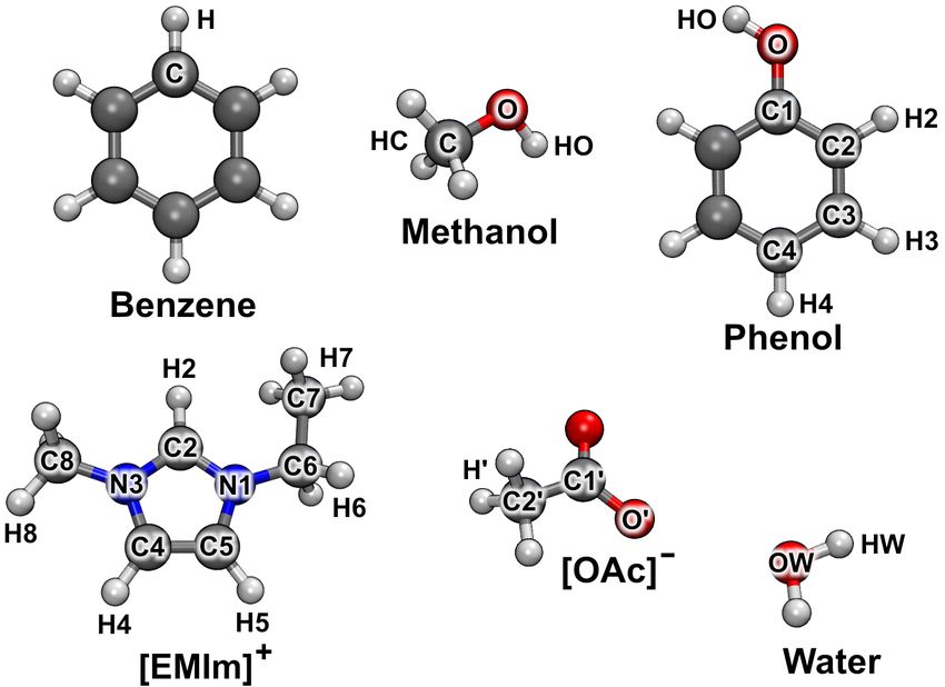
Molecules 2021, 26, 1875                                                                                            3 of 22

                           simulation should become minimal. With the aid of an optimization algorithm, this leads
                           to a rigorous definition of two sets of atomic radii, and it yields molecular charges as
                           well as atomic partial charges in bulk phase systems which are free of any empirical or
                           adjustable parameters.
                                 At the example of several simple organic compounds in the liquid phase, we will
                           show that the atomic partial charges obtained in this way are chemically reasonable and
                           can help to understand the specific interactions present in the systems, such as hydrogen
                           bonds [54,55]. Furthermore, the application to ionic liquid systems will reveal that the
                           ionic partial charges reflect the charge transfer effects (i.e., reduced ionic charges below
                           unity) that have been discussed for such systems [1–3,56–59]. In many force field molecular
                           dynamics studies of ionic liquids up to now, the ion charges have been empirically scaled
                           down to achieve this effect [1–3,57,58,60–62], which is required to obtain the correct time
                           scale of the dynamics. However, it has been recently shown that a simple scaling-down
                           procedure of atomic charges might break the subtle balance of interactions within such
                           complex systems [63]. We would like to mention that there exist also other studies which
                           have utilized different methods to obtain reduced ion charges without manual down-
                           scaling [63–67].
                                 The article is structured as follows: in Section 2, we give a general overview of our
                           novel method, followed by some in-depth details of the algorithms. In the next section,
                           the application of the method to several example systems is described and the results are
                           discussed. Subsequently, we show that a simple one-step scheme without optimized radii
                           fails to produce reasonable results (Supporting Information). Finally, we investigate the
                           basis set dependence of our approach. After the computational details, we end the article
                           with a conclusion.

                           2. Description of the Method
                           2.1. General Workflow
                                 As stated in the introduction, the Voronoi tessellation has been used for the calculation
                           of atomic partial charges before. This is also true for several extensions of the Voronoi
                           tessellation which include atomic radii [38–41]. However, to the best of our knowledge, the
                           radical Voronoi tessellation has not been employed to derive atomic partial charges before.
                           Apart from this, the central piece (and the novelty) of the herein presented approach is
                           the use of two different sets of radii at the same time in our two-step scheme, and the
                           on-the-fly optimization of the atomic radii by minimization of the charge fluctuations. The
                           rationale behind this procedure is the assumption that molecular charges as well as atomic
                           partial charges from a proper partitioning of the electron density should stay approximately
                           constant during the scope of a simulation, and only fluctuate around an average value
                           for a system without significant charge transfer [68,69]. The radical Voronoi tessellation is
                           utilized as a partitioning scheme which requires some parameters to be set (i.e., the atomic
                           radii). Based on the assumption made above, the optimal set of parameters is obtained
                           when the variance of the charge distribution of atoms/molecules becomes minimal. In
                           this case, the tessellation scheme assigns the electron density to the atoms/molecules in a
                           natural way, such that the fluctuations in the charge become small. Therefore, our approach
                           is free of any empirical or adjustable parameter.
                                 The next step is to decide which radii to include into the set of parameters that is
                           optimized for minimal charge fluctuations. One possibility would be to consider only
                           element radii as parameters, and assume all atoms of a certain element type to bear the
                           same radius. However, this would contradict the nature of chemical bonding. It would
                           seem quite counter-intuitive to constrain, e.g., a carboxyl carbon atom to possess the
                           same atomic radius as a methyl carbon atom somewhere else in the molecule. On the
                           other hand, it is also not a good idea to include the radii of all individual atoms into
                           the set of optimization parameters, as atoms which are chemically equivalent should
                           probably bear the same radius. A bulk phase water simulation should require, e.g., only
                           two parameters to optimize, namely the oxygen radius and the hydrogen radius. Based
Molecules 2021, 26, 1875 4 of 22
on these considerations, our method groups chemically equivalent (strictly speaking:
topologically equivalent [70]) atoms together, and uses one atomic radius for each such group
as optimization parameter. Similarly, all atoms within one such group are considered to
have the same atomic partial charge on average, only influenced by temporal fluctuations.
The objective of the optimization problem is the charge variance. This can either
be defined as the average variance of the charge distribution of chemically equivalent
atoms (which is then called atomic charge variance), or as the average variance of the charge
distribution of equivalent molecules (being called molecular charge variance). In both cases,
the variance is evaluated over the simulation cell (iterating through equivalent atoms or
molecules) as well as over the number of snapshots considered. This can be written as
!
1 K 1 T Ni
Var := ∑
K i=1 TNi t∑ ∑ qi,t,j − µi
2
(1)
=1 j =1
with the average value µi given by
T Ni
1
µi : =
TNi ∑ ∑ qi,t,j , (2)
t =1 j =1
where T is the number of snapshots that are to be evaluated. In the case of the atomic
charge variance, K is the number of non-equivalent atom types in the system, Ni depicts
how many equivalent atoms of type i exist, and qi,t,j is the charge of the j-th atom of type
i in snapshot t. In the case of the molecular charge variance, similarly, K is the number
of non-equivalent molecule types in the system, Ni depicts how many molecules of type
i exist, and qi,t,j is the total charge of the j-th molecule of type i in snapshot t. When
presenting the results, the standard deviation σ is used instead√ of the variance in order to
have the numbers in units of charge, simply defined as σ := Var.
Following from these definitions, a minimization of the atomic charge variance will
lead to a tessellation scheme which distributes the electron density to the atoms of the
system in a natural way, not considering that there exist molecules at all. On the other
hand, the minimization of the molecular charge variance will yield a partitioning which
accurately describes the distribution of electron density to different molecules, but does
not account at all for the way how the density is distributed to the atoms within each
molecule. Since average atomic point charges as well as average molecular/ionic charges
are important quantities, both optimization problems are interesting for sure. However,
it would be desirable to obtain a method which addresses both problems simultaneously,
giving reasonable atomic point charges as well as meaningful molecular charges in one
pass. In order to minimize both the molecular and the atomic charge variance, we have
developed a two-step approach.
n o We first perform a radical Voronoi tessellation based on a
first set of atomic radii rMol to partition the total simulation cell into molecular volumes.
For each such molecular volume, we perform a second radical Voronoi tessellation with a
second set of atomic radii rAtom in order to obtain the atomic Voronoi cells. Both sets of
radii are optimized independently during the procedure.
Altogether, this leads to the schematic flowchart in Figure 1. We have implemented this
algorithm in our open-source program package TRAVIS [70,71], thus it is freely available
to the scientific community. The details of the implementation will be discussed in the
following sections.Molecules 2021, 26, 1875 5 of 22
Figure 1. Flowchart of the proposed two-step optimization algorithm which yieldsnoptimized
o
molecular and atomic partial charges as well as two sets of optimized atomic radii rMol and
Atom
r via minimization of the charge variance.
2.2. Voronoi Tessellation and Radical Voronoi Tessellation
The Voronoi tessellation [34] is a mathematical tool which partitions an Euclidean
space containing some points (Voronoi sites) into non-overlapping subsets. Each Voronoi site
corresponds to exactly one such subset (called Voronoi cell), which contains all points from
space which are closer to this Voronoi site than to any other Voronoi site. In mathematical
form, this is written as
n o
Ci := x ∈ Rn k x − p i k ≤ x − p j ∀ j ∈ {1 . . . k }, j 6 = i , i ∈ {1 . . . k }, (3)
where Rn stands for any Euclidean space with the norm k · k, in which k Voronoi sites, each
with position pi ∈ Rn , are given, and the Ci ⊆ Rn are the resulting Voronoi cells.
By considering atoms in three-dimensional space as Voronoi sites, this concept has
widely been applied in different fields of computational chemistry. To name a few advan-
tages of the method, the Voronoi tessellation of a set of atoms is uniquely defined and can
be calculated with moderate computational demands. The Voronoi tessellation can easily
be adopted to systems with periodic boundary conditions, and is therefore well suited for
bulk phase systems. Finally, the method does not possess any parameters to tune, and
therefore gives an unbiased and uniquely defined picture.
However, certain limitations do arise from the properties of the standard Voronoi
tessellation. As all atoms are treated in the same way, Voronoi polyhedra of light atoms like
hydrogen will on average have the same size as those around heavier atoms like iodine.
From a mathematical point of view, this is not a problem, but from a chemical perspective,Molecules 2021, 26, 1875 6 of 22
this is completely unreasonable. If, e.g., the electron density within the Voronoi cell of a
hydrogen atom is integrated, the hydrogen atom would always end up with a heavily
negative partial charge, because way too much electron density would be considered as
belonging to this hydrogen atom.
To overcome this problem, radii need to be introduced into the Voronoi tessellation,
allowing to treat different atom types differently. Several ways to do so have been proposed
(see the introduction). However, many of them suffer from problems such as the “vertex
error” [42,44] (i.e., holes in the tessellation) or a lack of general applicability to arbitrary
systems. Therefore, the radical Voronoi tessellation [44] (also termed “power diagram”
in the two-dimensional case) will be employed here. It is an extension of the classical
Voronoi tessellation, where a radius ri is assigned to each Voronoi site pi . This results in
the definition
n o
2
Cir := x ∈ Rn k x − pi k2 − ri2 ≤ x − p j − r2j ∀ j ∈ {1 . . . k }, j 6= i , i ∈ {1 . . . k}. (4)
While in the classical case the face between two adjacent Voronoi cells is always placed
in the middle between the corresponding Voronoi sites, its position is now determined by
the difference of the squared radii. From Equation (4), it can be derived that the separation
plane between two sites A and B with radii rA and rB will be located at a position
2 − r2
1 rA B
w := + RAB , (5)
2 2R2AB
where RAB is the distance between both sites, and w describes the distance of the separation
plane from A—see Figure 2. It can be seen that the relative position of the plane depends
on the distance between the sites: if the distance becomes large with respect to the radii,
the plane will be located in the middle, even if the radii differ. In the other extreme case
of a small inter-site distance when compared to the radii, w can even be outside of the
interval [0, RAB ], which either means that one of the sites is no longer located inside of its
Voronoi cell, or the Voronoi cell of this site is degenerate (empty). However, both cases
are not a problem if electron density shall be integrated within the cells. These effects are
more pronounced if the differences between the radii become larger. If all radii are equal,
the radical Voronoi tessellation becomes identical to the classical Voronoi tessellation, and
those degeneracies cannot occur. A two-dimensional schematic illustration of the radical
Voronoi tessellation in the case of benzene is shown in Figure 3. Please note that the term
“radical” is not related to chemical radicals (which possess unpaired electrons).
Figure 2. Separation plane between two Voronoi sites A and B with radii rA and rB in the radical
Voronoi tessellation, see Equation (5).
The definition of the radical Voronoi tessellation in Equation (4) shows
that the tessel-
lation will not change if the set of radii ri is transformed to a new set ri0 by the map
q
ri0 := ri2 + C, i ∈ {1 . . . k} (6)Molecules 2021, 26, 1875 7 of 22
with some constant C ∈ R. Due to this relation, the absolute value of the radii does not
have a direct meaning, and one degree of freedom drops out of the optimization problem
described below.
Figure 3. Schematic two-dimensional illustration of the radical Voronoi tessellation in the bulk phase
of benzene. The solid black lines are iso-lines of the electron density, the dashed circles indicate the
atomic radii, and the radical Voronoi cells are shown as gray solid lines with the resulting molecular
boundaries drawn
n oin blue. The position of the blue lines is exclusively determined by the first set of
atomic radii rMol , while the position of the gray lines is solely determined by the second set of
radii rAtom .
In the TRAVIS implementation of the method presented herein, the Voro++ library [72,73]
from Chris Rycroft is used to perform the radical Voronoi tessellation of periodic simula-
tion cells, which may have the shape of any parallelepiped (therefore not restricting our
implementation to orthorhombic cells).
2.3. Integrating over Voronoi Cells
After the construction of the Voronoi cells, the electron density needs to be integrated
within each Voronoi cell and the core charge has to be added to yield the partial charge
of the corresponding atom. As the electron density in the simulation box is supplied on a
grid, an efficient algorithm is required to traverse the grid points which are located inside a
given Voronoi cell. A simplistic approach that checks for each grid point in which cell it is
located would lead to very poor performance, as there are around 10 million grid points
per snapshot (see Table 1). Instead, we have implemented another method: the three stride
vectors of the grid are termed v1 , v2 , v3 in the following. As non-orthorhombic simulation
cells are permissible, these vectors do not need to be orthogonal to each other. At first, the
maximum cross section of the Voronoi cell along the v1 direction is computed in the v2 –v3
plane. A (in the case of orthorhombic simulation cells) rectangular bounding box in that
plane is constructed around this section. For each grid coordinate pair within this bounding
box in the v2 –v3 plane, a ray is cast into v1 direction, and intersections between this ray
and all Voronoi faces of the given Voronoi cell are probed. As Voronoi cells are alwaysMolecules 2021, 26, 1875 8 of 22
convex, there may be either zero or two such ray–face intersections, other combinations are
not possible. With zero intersections, the ray misses the Voronoi cell, and no further action
is taken. With two intersections, the entry and exit points of the ray through the Voronoi
cell are known, and the grid points between the intersections can be summed up along
the ray. This algorithm finally yields the sum over all grid points located within the given
Voronoi cell. As each grid point is assigned to exactly one Voronoi cell by this algorithm,
the total sum over all Voronoi cells is equal to the total sum over all grid points, which is
important to keep the total charge of the system fixed. This implementation has already
been applied several times to obtain the electric dipole moments of molecules in bulk phase
simulations [45,52,53]. Our approach is rather efficient—a full Voronoi integration of a bulk
phase snapshot with around 1000 atoms and 10 million grid points takes roughly 1 s on a
single CPU core.
Table 1. Exemplary liquid phase simulations to which the method is applied, including composition,
orthorhombic cell vector, density, simulation temperature, and total electron density volumetric
grid resolution.
System Composition Cell/pm Density/g cm−3 Temp./K Grid Resolution
Benzene 32 benzene 1690 0.860 350 192 × 192 × 192
Methanol 48 methanol 1515 0.735 350 180 × 180 × 180
Phenol 32 phenol 1688 1.040 400 192 × 192 × 192
36 [EMIm]+
IL 2121 1.066 350 240 × 240 × 240
36 [OAc]−
27 [EMIm]+
ILW 27 [OAc]− 2158 1.000 350 243 × 243 × 243
81 H2 O
In real-world applications, the grid of the electron density is relatively coarse in order
to reduce the required storage space for the volumetric data. Typical values are in the order
of one grid point each 10 . . . 20 pm. As each grid point is completely assigned to exactly one
Voronoi cell, infinitesimal changes in the radii may lead to grid points switching the cell
they are assigned to. Therefore, the map from atomic radii to atomic charges is no longer
continuous, or in other words, some amount of numerical discretization noise is introduced,
which hampers the optimization algorithm for the radii. To reduce the impact of this effect,
we have developed and implemented an on-the-fly interpolation scheme for the electron
density grid. During the integration pass, the grid can be refined via tri-linear interpolation.
The smaller grid spacing which results from this procedure leads to a reduced amount of
numerical noise. On the other hand, demands on storage system and core memory are
not increased, as the interpolation is just performed on-the-fly while integrating. We call
this approach refinement; it has been utilized in all applications of our method presented
herein with a refinement factor of 2 (i.e., one grid point was interpolated to two grid points
along each axis of the grid, yielding 8 grid points in total from each original grid point).
Our implementation is not limited to a refinement factor of 2; higher values can be chosen
on demand.
2.4. Charge Variance Minimization Algorithm
As the objective function of the optimization problem to be solved is the charge vari-
ance in dependence of the atomic radii for the radical Voronoi tessellation of an arbitrarily
complex chemical system, it is easy to see that analytic expressions for the first derivatives
or for the Hessian of the objective with respect to the radii are not available. Therefore, the
gradient needs to be determined by numerical differentiation with respect to all radii by
following a finite-difference scheme. Unfortunately, the objective function is not strictly
continuous due to numerical noise introduced by the Voronoi tessellation and the discrete
grid of the electron density (see Section 2.3). A simple one- or two-sided finite differenceMolecules 2021, 26, 1875 9 of 22
approach therefore did not yield reliable gradients. Thus, our current implementation takes
three equidistant samples of the objective function on each side, giving a total amount
of seven samples (including the central position). A linear regression is performed on
these points, and the point which deviates most from the regression equation is removed.
On the remaining six points, another linear regression is performed, and the slope of the
resulting function is used as the gradient along this direction. This procedure is repeated
for each parameter of the optimization problem, i.e., each type of non-equivalent atoms.
The maximum displacement of each parameter was chosen to be 0.15 pm in each direction.
Based on this algorithm for the gradient calculation, a numerical optimization scheme
can be set up. We have decided to utilize the non-linear conjugate gradient (CG) method [74]
in combination with golden-section bracketing line search [75,76] due to the robustness and
resilience of this approach. There exist several flavors of the nonlinear conjugate gradient
method. Our implementation utilizes the Polak–Ribiére formula [77,78] to obtain the CG
mixing parameter β according to
rkT+1 (rk+1 − rk )
β k := , (7)
rkT rk
which yields better convergence rates than the original Fletcher–Reeves formula [74] in
many cases. If the value of β becomes negative, the usual approach to perform a downhill
step instead in order to reset the conjugate-gradient scheme has been implemented. Due to
the strong numerical noise, another measure is necessary: If the line search returns a step
which would increase the objective, this step is rejected, and the line search bracketing is
repeated with a reduced initial search interval. If the search interval falls below some small
threshold, a downhill step with line search is attempted. If this still does not reduce the
objective for more than a given threshold, the optimization is considered to be converged.
As
n initial
o radii for the optimization, we used van der Waals element radii [46–48] for
Mol
Atom
r and covalent element radii [79] for r . Since these radii are expected to
yield already a reasonable partition of the electron density between molecules and atoms,
respectively, the optimal radii should not be vastly different. This choice therefore reduces
the number of optimization steps and thus the required computer time. For an optimization
problem which possesses only one minimum, the choice of initial values does not influence
the results at all. For the simple example of methanol, it is discussed in Section 3.1 and
visualized in Figure 5 that there is only one charge variance minimum for the separation of
the molecular electron density, which is not far from the van der Waals radii.
3. Results and Discussion
In order to discuss some results of our proposed method, it has been applied to
several ab initio molecular dynamics simulations. Five trajectories of different liquid phase
simulations are evaluated within this work, see Table 1. The last two systems contain ion
pairs of the ionic liquid 1-ethyl-3-methylimidazolium acetate, abbreviated as [EMIm][OAc].
These two trajectories have been published and discussed in the literature before [50,80–82].
The atom nomenclature within the studied molecules is described in Figure 4. In the
following, the results from the analysis of the five example systems are presented.Molecules 2021, 26, 1875 10 of 22
Figure 4. Atom labeling of the molecules studied. Element colors: gray—carbon, red—oxygen,
blue—nitrogen, white—hydrogen.
3.1. Molecular Charges
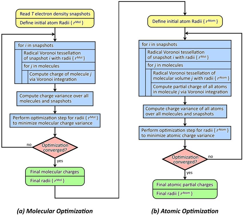
To visualize the optimization problem in the case of molecular charge fluctuations,
a contour plot of the standard deviation of the molecular charge in dependence of the
Voronoi radii is given in Figure 5 for the methanol system. In methanol, there are four
different types of atoms, and therefore, three degrees of freedom remain after factoring
out the invariance from Equation (6), namely the three differences rHC 2 − r2 , r2 − r2 ,
HO HC C
2 2
and rHC − rO . In order to arrive at a two-dimensional function for the sake of illustration,
the additional constraint rHC = rHO = rH has been applied here, which only concerns the
contour plot, and is in contrast to the computations performed in the remainder of this
section, were rHC and rHO are independent parameters. This leaves only two differences
of squared radii as degrees of freedom. The plot in Figure 5 shows that there exists a
well-defined minimum of the standard deviation of the molecular charge, which is close to
the van der Waals radii of the atoms, as it is already expected from the discussion in the
introduction. The point in the origin of the plot—which corresponds to the classical non-
radical Voronoi tessellation—possesses a significantly larger molecular charge fluctuation.
For large absolute values of the differences, stationary states are reached where no further
changes appear. In these situations, the Voronoi cells of the atoms with the smaller radius
completely vanish, so these atoms do no longer appear in the tessellation at all. In the
upper right corner of the plot, only the hydrogen atoms possess a Voronoi cell, while only
the carbon atoms remain in the upper left corner, and the tessellation just contains the
oxygen atoms in the lower right corner. Consequently, the carbon atoms disappear in the
valley to the right side, the oxygen atoms vanish in the valley to the top, and the hydrogen
atoms do not have a cell in the valley to the lower left corner. The deepest valley is the one
leading to the right side, indicating that it is most important to correctly place the cell faces
between hydrogen and oxygen atoms for a reasonable distribution of the electron density
to the methanol molecules.Molecules 2021, 26, 1875 11 of 22
Figure 5. Standard deviation of the charge distribution in the methanol system as a function of the
Voronoi radii (assuming rHC = rHO = rH here). The σ values are given in units of e. The black cross
marks the van der Waals radii [46–48].
The molecular charges that were obtained by applying the proposed optimization
algorithm are given in Table 2. For the non-ionic systems which contain only one molecule
type (benzene, methanol, phenol), it is clear by definition that the average molecular charge
always has to be zero. For these systems, only the standard deviation of the charge is of
interest. We find that the standard deviation of the molecular charge is quite small in all
cases, in the range of 0.01 e. This indicates that the electron density is well partitioned to
the individual molecules, so that each molecule is close to its expected average charge of
zero in every configuration.
Table 2. Resulting average molecular charges and corresponding standard deviation for the five
simulations from Table 1. All numbers in units of e.
Molecule Charge Std. Dev.
Benzene 0 0.010
Methanol 0 0.013
Phenol 0 0.012
IL
[EMIm]+ 0.846 0.016
[OAc]− −0.846 0.011
ILW
[EMIm]+ 0.859 0.017
[OAc]− −0.817 0.015
Water −0.014 0.015
When considering the pure ionic liquid system (IL), all observations concerning the
standard deviation of molecular charges from above still hold. More interesting, the ionic
charges are found to be within a range of 0.8 e . . . 0.85 e. It has been shown before that
ion charges of approximately 0.8 e lead to a good reproduction of experimental quantities
in classical molecular dynamics simulations [1,2,56,57]. In many force field molecularMolecules 2021, 26, 1875 12 of 22
dynamics studies of ionic liquids up to now, the ion charges have been empirically scaled
down to achieve this effect [1–3,57,60–62], which is no longer required with our approach.
The finding that average charges of anion and cation equal each other in absolute value
follows by definition from the charge neutrality of the simulation box.
Finally, there are some interesting points to note for the ionic liquid/water mixture
(ILW). The charge neutrality of the system is also fulfilled in this case—please note that the
average ionic/molecular charges need to be multiplied with the number of ions/molecules
in order to sum up to zero (see Table 1). The cation charge becomes larger by the addition of
water, whereas the anion charge becomes smaller in absolute value. Therefore, the absolute
value of the cation charge is on average larger than that of the anion charge, and the water
molecules possess a small negative charge on average (however, smaller than the standard
deviation in absolute value). These findings indicate that the water molecules interact
more strongly with the anions than with the cations, as this explains both observations:
Cations become even more positive due to missing hydrogen bonds to the acetate, as most
acetate hydrogen bond acceptors are occupied by water molecules now. Acetate anions
become less negative on average, as they can form much more and stronger hydrogen
bonds to water molecules (imidazolium cations are fairly weak hydrogen bond donors in contrast
to water). These relations have already been observed in earlier articles about this ionic
liquid by using a different methodology [62,80,81]. Thus, the molecular charges obtained
by our method even provide some insights into the chemistry and binding affinity of the
compounds of a mixture.
3.2. Atomic Partial Charges and Radii
In this section, the atomic partial charges as well as the two sets of optimized radii
rMol and rAtom which have been obtained from the analysis of the example systems will be
discussed, see Tables 3 and 4 (the results are split over two tables for better readability).
Table 3. Resulting atomic partial charges, standard deviations as well as molecular and atomic
Voronoi radii for the first three systems from Table 1. Charges and standard deviations in units of e,
radii in pm. For atom labels, see Figure 4.
Atom Charge Std. Dev. r Mol r Atom
Benzene
C 0.141 0.007 173.7 72.9
H −0.141 0.010 107.6 41.8
Methanol
C 0.764 0.008 172.5 76.4
HC −0.169 0.010 112.9 51.7
O −0.609 0.023 152.9 81.1
HO 0.350 0.026 104.0 28.8
Phenol
C1 0.248 0.014 170.1 73.8
C2 0.084 0.013 172.8 73.9
C3 0.154 0.010 171.6 72.9
C4 0.122 0.012 173.2 72.8
H2 −0.115 0.011 107.9 41.3
H3 −0.134 0.011 111.5 41.5
H4 −0.130 0.011 111.4 40.4
O −0.447 0.025 152.9 78.0
HO 0.229 0.024 104.3 39.2
In case of the benzene system, there are only two non-equivalent atom types. Much
electron density of the benzene molecules is assigned to the carbon atoms, so the hydrogen
atoms bear a positive charge of around +0.14 e. The standard deviation of the atomic
charges is around 0.01 e and therefore quite small, indicating a reasonable partitioning of
the electron density to the individual atoms. Considering the optimized radii, we find thatMolecules 2021, 26, 1875 13 of 22
hydrogen possesses a significantly smaller radius than carbon in both sets, as it would be
expected from chemical intuition. The radii from molecular charge optimization are larger
than those from atomic charge optimization, similarly to van der Waals radii [46–48] being
larger than covalent radii [79].
Table 4. Resulting atomic partial charges, standard deviations as well as molecular and atomic Voronoi radii for the final
two systems from Table 1. Charges and standard deviations in units of e, radii in pm. For atom labels, see Figure 4.
IL ILW
Atom
Charge Std. Dev. r Mol r Atom Charge Std. Dev. r Mol r Atom
[EMIm]+
N1 −0.306 0.011 167.3 82.7 −0.316 0.011 162.2 80.8
C2 0.270 0.015 165.2 79.5 0.350 0.015 160.1 76.9
N3 −0.223 0.013 163.7 80.3 −0.294 0.011 168.3 80.1
C4 0.149 0.014 169.1 78.0 0.254 0.014 168.1 74.8
C5 0.148 0.013 169.1 78.7 0.219 0.013 171.9 75.7
C6 0.468 0.009 172.3 73.5 0.541 0.008 170.3 71.7
C7 0.518 0.007 171.4 71.4 0.455 0.007 178.0 71.9
C8 0.655 0.010 165.2 72.0 0.688 0.008 163.5 71.4
H2 0.092 0.025 107.3 37.3 0.055 0.022 108.0 36.3
H4 0.041 0.022 106.9 38.2 −0.025 0.018 105.1 40.8
H5 −0.093 0.019 107.3 39.8 −0.124 0.015 109.8 40.8
H6 −0.092 0.020 107.3 39.8 −0.123 0.015 109.8 40.8
H7 −0.156 0.015 109.6 41.6 −0.139 0.014 105.9 40.2
H8 −0.115 0.019 108.9 41.7 −0.125 0.014 110.1 42.1
[OAc]−
C1’ 0.761 0.015 162.4 73.4 0.882 0.018 165.2 72.7
C2’ 0.482 0.008 175.2 71.7 0.414 0.008 175.2 73.5
H’ −0.162 0.011 109.8 41.1 −0.138 0.011 109.1 41.8
O’ −0.801 0.020 155.5 83.1 −0.849 0.024 155.6 85.0
Water
OW −0.553 0.024 155.8 79.2
HW 0.269 0.025 108.1 36.0
Concerning the methanol simulation, it can be seen that the oxygen atom bears a
significantly negative charge of −0.61 e, while the hydroxyl proton is positively charged
with +0.35 e, leading to a strong dipole in the hydroxyl group as expected. The central
carbon atom is very positive with a charge of +0.76 e, while the aliphatic protons are
negative at around −0.17 e. The standard deviation in the charges of the carbon and
aliphatic hydrogen atoms is small, while that of the oxygen and hydrogen atoms from the
hydroxyl group is larger by a factor of 2 . . . 3. This is due to the strong hydrogen bond
which can be formed between hydroxyl groups: if a hydrogen bond is present, the atomic
charges will be different due to a certain amount of charge transfer, so that the standard
deviation is larger. An increased standard deviation of an atomic charges is therefore an
indication for a strong directed interaction involving this atom. For the atom radii, we
find that the hydroxyl proton possesses by far the smallest value, significantly smaller
than that for the aliphatic hydrogen atoms. This nicely shows how our approach assigns
different radii to atoms of the same element, depending on their chemical environment and
bonding situation. It also confirms our decision to vary the radii of non-equivalent atoms
individually in the optimization procedure (rather than treating all atoms of one element with
the same radius).
For the phenol simulation, the picture becomes slightly more complex, as we have
nine non-equivalent types of atoms now. As expected, the hydroxyl oxygen atom bears a
significantly negative charge of −0.45 e, while the hydroxyl proton is positive with +0.23 e.
The aromatic C1 carbon atom is significantly positive due to the electron-withdrawing
effect of the hydroxyl group. It is very interesting to note that we find an alternatingMolecules 2021, 26, 1875 14 of 22
“positive–negative–positive–negative” charge pattern (relatively to the average carbon charge
of +0.14 e) when going from C1 to C4 which attenuates with rising distance from the
hydroxyl group. This alternating pattern is well known in aromatic chains and rings, and
is an important cause of the regioselectivity in aromatic reactions. Also here, the standard
deviation of the oxygen and hydrogen atom of the hydroxyl group is significantly larger
than the value of all other atoms, indicating a strong directed interaction, which is again a
hydrogen bond.
In the pure ionic liquid system (IL), some interesting observations can be made.
The most positive hydrogen atom is the central ring proton H2, which is known to be a
hydrogen bond donor [62,80–84]. The other two ring protons H4 and H5 are significantly
less positive. H5 even is assigned a slight negative charge of −0.09 e, which certainly is
an unexpected result. A significant amount of the positive charge is concentrated in the
two side chains of the ion, while the ring only possesses a slight positive charge of around
+0.1 e in total. In acetate, the oxygen atoms bear a strong negative charge as expected,
while the carboxyl carbon atom is significantly positive. Concerning the standard deviation
of the atomic charges, the observation from above holds: strong hydrogen bonds exist
between the ring protons H2, H4, and H5 and the acetate oxygen atoms O’, and these four
atoms also possess the largest standard deviation in their charge due to the charge transfer
effect of the hydrogen bond.
When going to the mixture of the ionic liquid with water (ILW), most observations
from the last paragraph still hold. The central ring proton H2 becomes slightly less positive
when water is added (i.e., water depolarizes the [EMIm]+ cation), while the acetate oxygen
atoms become even more negative due to the water addition (i.e., water polarizes the [OAc]−
anion). This is exactly what was observed in literature before from AIMD simulations of
this mixture [80]. It is interesting to note that the charge distribution within the water
molecules yields qOW = −0.55 e, which indicates a slightly weaker charge separation than
in popular three-site water force fields, like, e.g., qOW = −0.85 e in SPC/E [85]. This might
be due to the fact that the hydrogen bond network of water is interrupted by the ionic
liquid—in particular by the almost non-polar cation—so that water molecules become
depolarized in the vicinity of [EMIm]+ as observed before [80].
Based on these considerations, it can be stated that the atomic charges and radii
obtained by our two-step approach are helpful for understanding the relevant interactions
in liquid-phase systems. Strong directed interactions can be identified by an increased
standard deviation of the atomic charge due to the charge transfer effect. In phenol, the
alternating charge pattern induced by the hydroxyl substituent could be well observed,
so that our charges are able to predict reactivity and regioselectivity in aromatic systems.
Finally, the optimized atomic radii show a significant distinction between atoms of the
same element—for example, protic hydrogen atoms such as the [EMIm]+ ring protons
and the hydroxyl protons are assigned a smaller radius than aliphatic hydrogen atoms,
and can thus be identified in a bulk phase simulation. Therefore, our optimized radii are
more flexible than van der Waals [46–48] or covalent [79] atom radii from literature, which
possess fixed values per element.
In order to show that our two-step Voronoi integration scheme with optimized radii
is indeed worth the effort, we have computed the Voronoi charges for the five systems
from Table 1 of the manuscript via a one-step Voronoi integration with three different
sets of non-optimized standard radii. The results are presented in Tables S1–S4 in the
Supplementary Materials, where we also discuss the values. In summary, we demonstrate
there that a single set of radii in the radical Voronoi tessellation is not able to describe both
the separation between individual molecules and the partitioning of the molecular electron
density to the atoms well at the same time. If both shall be described in a reasonable way,
two different sets of radii need to be employed simultaneously, as we do in our two-step
approach which is presented here.Molecules 2021, 26, 1875 15 of 22
3.3. Basis Set Dependence
When considering methods for computing atomic partial charges via electron structure
theory, a very important quantity is the basis set dependence of the method. While methods
which directly evaluate the molecular orbitals (such as Mulliken and Löwdin charges) are
typically very sensitive with respect to the choice of the basis set, methods which only rely
on the total electron density (such as RESP and Hirshfeld charges) are often more robust and
show less dependence.
To investigate the basis set dependence of our approach, we have re-calculated the
snapshots for the ILW system with three different basis set sizes (MOLOPT-SZV-SR,
MOLOPT-DZVP-SR, MOLOPT-TZVPP-SR) [86] and used the electron densities result-
ing from these calculations to compute our two-step Voronoi charges. The size of the three
basis sets differs considerably. While the SZV basis possesses only 0.87 basis functions
per electron in the case of the ILW system, the DZVP basis set possesses 3.21 functions
per electron, and the TZVPP basis set even 5.54 functions per electron for this system
(13,770 functions in total). As all our calculations are restricted Kohn–Sham calculations,
electrons are considered as pairs, so that values of less than one basis function per electron
are possible (a minimal basis set would have 0.5 functions per electron in an RKS calculation).
The results from our calculations are presented in Table 5 and as a diagram in Figure 6.
At first sight, it can be seen that the basis set dependence is relatively small, and the
optimized atomic partial charges qualitatively agree with all three basis sets. When going
from SZV to DZVP, there are slightly larger changes for some atom types. This can be easily
understood from the fact that the SZV basis set is tiny (with only 0.87 basis functions per
electron), and is just not able to describe the electron structure of the system in a reasonable
way. Between DZVP and TZVPP, the agreement is better, except for the two carbon atoms
of acetate C1’ and C2’. When comparing SZV to TZVPP, the average deviation between
atomic charges is 0.04 e, while for DZVP to TZVPP it is only 0.02 e. This is in the range
of the standard deviation of the atomic charges obtained by our approach (see Tables 3
and 4), and therefore completely satisfactory. We can therefore conclude that the basis set
dependence of our two-step Voronoi charge approach is small, similar to other methods for
computing charges which only rely on the total electron density.
Figure 6. Influence of the basis set size on the optimized atomic partial charges in the ILW simulation.
Vertical axis in units of e. For atom labels, see Figure 4.Molecules 2021, 26, 1875 16 of 22
Table 5. Optimized molecular and atomic partial charges as well as corresponding standard devia-
tions for the ILW simulation with three different basis set sizes. All numbers in units of e. For atom
labels, see Figure 4.
SZV DZVP TZVPP
Atom
Charge Std. Dev. Charge Std. Dev. Charge Std. Dev.
[EMIm]+ 0.948 0.015 0.859 0.017 0.841 0.018
N1 −0.331 0.010 −0.316 0.011 −0.313 0.011
C2 0.352 0.015 0.350 0.015 0.382 0.015
N3 −0.280 0.011 −0.294 0.011 −0.307 0.011
C4 0.241 0.014 0.254 0.014 0.257 0.014
C5 0.158 0.014 0.219 0.013 0.220 0.013
C6 0.395 0.009 0.541 0.008 0.515 0.008
C7 0.461 0.008 0.455 0.007 0.513 0.007
C8 0.619 0.009 0.688 0.008 0.705 0.008
H2 0.072 0.022 0.055 0.022 0.038 0.021
H4 0.031 0.019 −0.025 0.018 −0.033 0.018
H5 −0.057 0.014 −0.124 0.015 −0.119 0.015
H6 −0.057 0.014 −0.123 0.015 −0.118 0.015
H7 −0.128 0.013 −0.139 0.014 −0.157 0.014
H8 −0.093 0.013 −0.125 0.014 −0.131 0.014
[OAc]− −0.909 0.016 −0.817 0.015 −0.797 0.015
C1’ 0.711 0.018 0.882 0.018 0.791 0.015
C2’ 0.378 0.009 0.414 0.008 0.506 0.008
H’ −0.132 0.010 −0.138 0.011 −0.164 0.011
O’ −0.800 0.028 −0.849 0.024 −0.801 0.024
Water −0.013 0.014 −0.014 0.015 −0.015 0.015
OW −0.565 0.027 −0.553 0.024 −0.553 0.023
HW 0.276 0.029 0.269 0.025 0.269 0.025
4. Computational Details
All simulations have been carried out with the program package CP2k [87–89], us-
ing the Quickstep module [90] in conjunction with the orbital transformation (OT) algo-
rithm [91]. The electron structure was calculated by density functional theory [92,93], using
the BLYP functional [94,95] together with the recent re-parametrization [96] of Grimme’s
D3 dispersion correction [97,98] with Becke–Johnson damping. Basis sets of the kind DZVP-
MOLOPT-SR [86] together with Goedecker–Teter–Hutter (GTH) pseudopotentials [99–101]
have been applied. The plane wave cutoff was set to 350 Ry with a REL_CUTOFF of 40.
The temperature during the simulations was kept constant using a Nosé–Hoover chain
thermostat [102–105] with a time constant of 100 fs. The integration time step was set to
0.5 fs in all cases.
For the benzene, methanol, and phenol systems, the initial configurations were created
with the Packmol software [106]. A force field pre-equilibration with OPLS–AA force field
parameters [107] was performed using LAMMPS [108]. These three simulations have
been equilibrated for some picoseconds with massive thermostating before the start of
the production run. The IL and ILW systems were restarted from the last snapshot of the
AIMD trajectories which were already published in literature [80–82]. Please note that
[EMIm][OAc] refers to the ionic liquid 1-ethyl-3-methylimidazolium acetate [80–82].
The electron densities of the simulation cells have been written to disk as volumetric
data with a grid spacing of approximately 10 pm, yielding typical grid resolutions of
around 240 × 240 × 240 for the large systems. A snapshot of the electron density was
written every 1000 time steps (i.e., every 0.5 ps) and compressed in our recently published
bqb format [109], which is now directly available in CP2k and yields a lossless compression
ratio of around 40:1, so that the storage requirements became tractable. 32 such snapshots
have been evaluated for each system, sampling 16 ps of physical time. An on-the-flyMolecules 2021, 26, 1875 17 of 22
refinement factor of 2 (see Section 2.3 above) has been used for integrating the Voronoi cells
for all five systems. The determination of the factor value was based on the observation
that the charges seem to be well converged with a factor 2 in our applications, and larger
values no longer lead to significant changes in the results.
Figure 4 was created with VMD [110] and Tachyon [111], while Figure 5 has been
prepared with Gnuplot [112].
5. Conclusions
In this article, we presented a novel method for the calculation of optimized molecular
charges and atomic partial charges from bulk phase simulations, which is based on a two-
step radical Voronoi tessellation of the system and subsequent integration of the electron
density within each Voronoi cell. First, the total electron density
n is
o partitioned into the
contributions of each molecule by using a set of atomic radii rMol , while in the second
step, the electron density within each molecule is assigned to the individual atoms using a
second set of atomic radii rAtom . Both sets of radii are optimized on-the-fly to minimize
charge fluctuations of atoms and molecules. Therefore, our approach yields atomic partial
charges without any empirical parameters. Two sets of optimized atomic radii are obtained
as a by-product from each run. It should be noted that the absolute values of these radii
do not have a direct meaning, since only the differences of squared radii determine the
partitioning of the total space into molecular volumes and the partitioning of each molecular
volume into atomic cells. Nevertheless, these two sets of radii can be considered specialized
van der Waals and covalent radii, which resemble many properties and interactions in the
specific system investigated, and can be applied for further analysis. The ability to handle
periodic systems—including non-orthorhombic cells—makes the method particularly well
suited for the application to bulk phase systems such as simulations of liquids. Only the
total electron density distribution on a grid is required as input data. Therefore, our method
is not limited to Hartree–Fock or DFT, and can be easily combined with all electronic
structure methods that are able to provide the total electron density on a real-space grid,
such as orbital-free approaches [113], DFTB [114–118], multi-reference calculations, or even
MP2 [119,120] and coupled-cluster methods [121–123]. With our recently published lossless
compression algorithm for electron density trajectories (“bqb format”, [109]) which yields
a lossless compression ratio of around 40:1, the storage requirements of this data along a
simulation trajectory become tractable.
In the second part of the article, we applied the newly developed method to five bulk
phase simulations of organic molecules and ions and discussed the results. The standard
deviations of the molecular and atomic charges are around 0.01 e and therefore very small,
which indicates a reasonable partitioning of the total electron density to the molecules and
atoms. We show that the optimized charges and radii obtained by our approach are useful
to understand the interactions in the system. For example, strong directed interactions
such as hydrogen bonds can be detected by an increased charge standard deviation of the
involved atoms. In the case of phenol, we find the typical alternating charge pattern in the
aromatic system that is induced by the hydroxyl substituent, so that our charges can even
be used to predict reactivity and regioselectivity in aromatics. From the application to bulk
phase ionic liquid systems, it was shown that the well-known reduction of ionic charge
below unity [1–3,56–59] is reproduced, predicting ion charges in the range of 0.8 . . . 0.85 e
without any empiricism, tuning, or constraints. In many force field molecular dynamics
studies of ionic liquids up to now, the ion charges have been empirically scaled down
to achieve this effect [1,2,60–62], which is required to obtain the right time scale for the
dynamics. However, it has been recently shown that a simple scaling-down procedure
of atomic charges might break the subtle balance of interactions within such complex
systems [63]. With our approach, such a down-scaling is unnecessary, as the resulting ion
charges are already within the range of values that have been shown do yield realistic
dynamics [1–3,56–59]. Apart from that, we have demonstrated that the use of either van
der Waals or covalent radii in a one-step Voronoi integration (using only one set of radii)You can also read