Morphology of three-body quantum states from machine learning
←
→
Page content transcription
If your browser does not render page correctly, please read the page content below
PAPER • OPEN ACCESS

Morphology of three-body quantum states from machine learning
To cite this article: David Huber et al 2021 New J. Phys. 23 065009

View the article online for updates and enhancements.

                               This content was downloaded from IP address 46.4.80.155 on 11/09/2021 at 23:02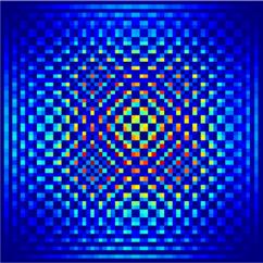
New J. Phys. 23 (2021) 065009                                                               https://doi.org/10.1088/1367-2630/ac0576

                                 PAPER

                                 Morphology of three-body quantum states from machine
O P E N AC C E S S
                                 learning
R E C E IVE D
3 March 2021
                                 David Huber1 , Oleksandr V Marchukov2 , Hans-Werner Hammer1 , 3 , ∗                        and
R E VISE D
21 May 2021                      Artem G Volosniev4
                                 1
AC C E PTE D FOR PUBL IC ATION       Technische Universität Darmstadt, Department of Physics, Institut für Kernphysik, 64289 Darmstadt, Germany
                                 2
26 May 2021                          Technische Universität Darmstadt, Institut für Angewandte Physik, Hochschulstraße 4a, 64289 Darmstadt, Germany
                                 3
PUBL ISHE D
                                     ExtreMe Matter Institute EMMI and Helmholtz Forschungsakademie Hessen für FAIR (HFHF), GSI Helmholtzzentrum für
23 June 2021                         Schwerionenforschung GmbH, 64291 Darmstadt, Germany
                                 4
                                     Institute of Science and Technology Austria, Am Campus 1, 3400 Klosterneuburg, Austria
                                 ∗
                                     Author to whom any correspondence should be addressed.
Original content from
this work may be used            E-mail: hans-werner.hammer@physik.tu-darmstadt.de
under the terms of the
Creative Commons                 Keywords: quantum billiards, machine learning, impurity systems, quantum chaos
Attribution 4.0 licence.
Any further distribution
of this work must
maintain attribution to          Abstract
the author(s) and the
title of the work, journal       The relative motion of three impenetrable particles on a ring, in our case two identical fermions
citation and DOI.                and one impurity, is isomorphic to a triangular quantum billiard. Depending on the ratio κ of the
                                 impurity and fermion masses, the billiards can be integrable or non-integrable (also referred to in
                                 the main text as chaotic). To set the stage, we first investigate the energy level distributions of the
                                 billiards as a function of 1/κ ∈ [0, 1] and find no evidence of integrable cases beyond the limiting
                                 values 1/κ = 1 and 1/κ = 0. Then, we use machine learning tools to analyze properties of
                                 probability distributions of individual quantum states. We find that convolutional neural networks
                                 can correctly classify integrable and non-integrable states. The decisive features of the wave
                                 functions are the normalization and a large number of zero elements, corresponding to the
                                 existence of a nodal line. The network achieves typical accuracies of 97%, suggesting that machine
                                 learning tools can be used to analyze and classify the morphology of probability densities obtained
                                 in theory or experiment.

                                 1. Introduction

                                 The correspondence principle conjectures that highly excited states of a quantum system carry information
                                 about the classical limit [1]. In particular, it implies that there must be means to tell a difference between a
                                 ‘typical’ high-energy quantum state that corresponds to an integrable classical system from a ‘typical’
                                 high-energy state that corresponds to a chaotic system. A discovery of such means is a complicated task that
                                 requires a coherent effort of physicists, mathematicians, and philosophers [2–4]. Currently, there are two
                                 main approaches to study chaotic features in quantum mechanics. One approach relies on the statistical
                                 analysis of the energy levels of a quantum-mechanical system. Another focuses on the morphology of wave
                                 functions. These approaches led to a few celebrated conjectures that postulate features of energy spectra and
                                 properties of eigenstates [5–7]. The postulates are widely accepted now, thanks to numerical as well as
                                 experimental data [8, 9].
                                     Numerical and experimental data sets produced to confirm the proposed conjectures are so large that it
                                 is difficult, if not hopeless, for the human eye to find universal patterns beyond what has been conjectured.
                                 Therefore, it is logical to look for computational tools that can learn (with or without supervision) universal
                                 patterns from large datasets. One such tool is deep learning (DL) [10], which is a machine learning method
                                 that uses artificial neural networks (NNs) with multiple layers for a progressive learning of features from the
                                 input data. It requires very little engineering by hand, and can easily be used to analyze big data across
                                 disciplines, in particular in physics [11]. DL tools present an opportunity to go beyond the standard
                                 approaches of quantum chaologists [12]. For example, in this paper, NN built upon many states are used to

                                 © 2021 The Author(s). Published by IOP Publishing Ltd on behalf of the Institute of Physics and Deutsche Physikalische Gesellschaft
New J. Phys. 23 (2021) 065009                                                                         D Huber et al

analyze the morphology of individual wave functions. Therefore, DL provides us with means to connect and
extend tools already used to understand ‘chaos’ in quantum mechanics.
    Recent work [13] has already opened an exciting possibility to study the quantum–classical
correspondence in integrable and chaotic systems using DL. In particular, it has been suggested that a NN
can learn the difference between wave functions that correspond to integrable and chaotic systems. It is
important to pursue this research direction further, and to understand and interpret how an NN
distinguishes the two situations. This information can be used in the future to formulate new conjectures
on the role of classical chaos in quantum mechanics. The main challenge here is the extraction of this
information from an NN, which often resembles a black box. Ongoing research on interpretability of NNs
suggests certain routes to understand the black box [14–16] (see also recent works that discuss this question
for applications in physical sciences [17–19]). However, there is no standard approach to this problem. In
part, this is connected to the fact that DL relies on general-purpose learning procedures, therefore, one does
not expect that there can be a unique way to analyze a NN at hand. For example, as we will see, the training
of a network for the ‘integrable’ vs ‘chaotic’ state recognition is very similar to the classic dog-or-cat
classification5 . It is not clear, however, that the tools that can be used to interpret the latter (e.g., based on
stable spatial relationships [20]) are also useful for the former. In particular, a training set for the
‘integrable’-or-‘chaotic’ problem contains information about vastly different length scales (determined by
the energy), whereas a training set for cats vs dogs has only length scales given by the size of the animal.
Therefore, it is imperative to study interpretability of NNs used in physics separately from that in other
applications.
    In this paper we analyze a NN, which has been trained using highly excited states of a triangular billiard,
and attempt to extract the learned features. Billiards are conceptually simple systems, yet it is expected that
they contain all necessary ingredients for studying the role of chaos in quantum mechanics [8].
Furthermore, eigenstates of quantum billiards are equivalent to the eigenstates of the Helmholtz equation
with the corresponding boundary conditions, which connects quantum billiards and the wave chaos in
microwave resonators [8, 21]. The triangular billiard is one of the most-studied models in quantum
chaology [22–26], and therefore it is well-suited for our study focused on analyzing neural networks as a
possible tool for quantum chaology.
    In our analysis, we rely on convolutional neutral networks (ConvNets) for image classification [27],
which have recently been successfully applied to categorize numerical and experimental data in physical
sciences [13, 28–35]. These advances motivate us to apply ConvNets to categorize quantum states as
integrable and non-integrable. Our goal can be stated as follows: given a set of highly excited states, build a
network that can classify any input state as integrable or not, and, moreover, study features of this network.
One comment is in order here. There are various definitions of quantum integrability [36], so we need to be
more specific. In this work, we call a quantum system integrable, if it is Bethe-ansatz integrable, i.e., if one
can write any eigenstate as a finite superposition of plane waves. We shall also sometimes use the word
chaotic instead of non-integrable. Finally, we note that the properties ‘integrable’ and ‘non-integrable’ are
usually attached to a given physical system, e.g., following an analysis of global properties like the
distribution of energy levels. However, the correspondence principle implies that these labels can also be
applied to individual states of a quantum system. In this paper, we use both notions and show that they are
compatible. We employ NNs to analyze the wave functions of individual quantum states.
    We show that a trained network accurately classifies a state as being ‘integrable’ or ‘non-integrable’,
which implies that a ConvNet learns certain universal features of highly-excited states. We argue that a
trained NN considers almost any random state generated by a Gaussian, Laplace or other distribution as
‘chaotic’, as long as the state includes a sufficient amount of zero values. This observation agrees with our
intuition that a non-integrable state has only weak correlations. We discuss the effect of the noise and coarse
graining in our classification scheme, which sets limitations on the applicability of NN to analyze
experimental and numerical data.
    Our motivation for this work is thus threefold: first, we want to demonstrate that NNs can classify the
morphology of the three-body states correctly. Therefore, we investigate a known model system with two
identical fermions and an impurity as a function of the impurity mass in order to be able to verify the NN
analysis. Second, we want to analyze the classifying network and understand the way it operates. Our third
goal is to use the network analysis to clarify the situation regarding suggested new integrable cases for other
parameter values than the established ones [37, 38]. However, we do not find any evidence of such cases.
    The paper is organized as follows. In section 2 we introduce the system at hand: a triangular quantum
billiard that is isomorphic to three impenetrable particles on a ring. Its properties are discussed in section 3

5   This figure is generated by adapting the code from https://github.com/gwding/draw_convnet.

                                                       2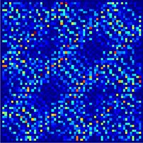
New J. Phys. 23 (2021) 065009                                                                                    D Huber et al

using standard methods. In section 4, we present our NN approach and use it in section 5 to classify the
states of the system. Moreover, we analyze the properties of the network. In section 6, we conclude. Some
technical details are presented in the appendix.

2. Formulation

We study billiards isomorphic to the relative motion of three impenetrable particles in a ring: two fermions
and one impurity. Characteristics of these triangular billiards are presented below, see also reference
[39, 40]. Our choice provides us with a simple parametrization of triangles in terms of the mass ratio,
κ = mI /m, where mI (m) is the mass of the impurity (fermions). Furthermore, it allows us to shed light on
the problem of three particles in a ring with broken integrability [41–43].
    For simplicity, we always assume that the impurity is heavier than (or as heavy as) the fermions,
corresponding to 1/κ ∈ [0, 1]. As we show below, this leads to a family of isosceles triangles with the
limiting cases (90◦ , 45◦ , 45◦ ) for 1/κ = 0 and (60◦ , 60◦ , 60◦ ) for κ = 1. These limiting triangles correspond
to two identical hard-core particles in a square well and a 2 + 1 Gaudin–Yang model on a ring [44],
respectively. Both limits are Bethe-ansatz integrable, see references [23, 45] for a more detailed discussion.
Note that certain extensions to the Bethe ansatz suggest that additional solvable cases exist [37, 38].
However, our numerical analysis does not find any traces of solvability beyond the two limiting cases, and
supports the widely accepted idea that almost any one-dimensional problem with mass imbalance is
non-integrable (notable exceptions are discussed in references [46–50]). Therefore, in this work we refer to
systems with 1/κ = 0 and 1 as integrable, in the sense that they can be analytically solved using the Bethe
ansatz (cf reference [36]). Systems with other mass ratios are called non-integrable.

2.1. Hamiltonian
The Hamiltonian of a three-particle system with zero-range interactions reads as

                                      2 ∂ 2    2 ∂ 2     2 ∂ 2
                                H=−         2 −       2 −        2
                                                                   +g   δ(xi − y).                                        (1)
                                      2m ∂x1    2m ∂x2    2κm ∂y      i

Everywhere below we focus on the limit g → ∞. In equation (1), 0 < xi < L (0 < y < L) is the coordinate
of the ith fermion (impurity), while L is the length of the ring, see figure 1(a). The eigenstates (φ) of H are
periodic functions in each variable. They are antisymmetric with respect to the exchange of fermions, i.e.,
φ(x1 , x2 , y) = −φ(x2 , x1 , y). Furthermore, the limit g → ∞ demands that φ vanishes when the fermion
approaches the impurity, i.e., φ(xi → y) → 0. For convenience, we use the system of units in which  = 1
and m = 1 in the following. For our numerical analysis, we choose units such that L = π.
    The Hamiltonian H can be written as a sum of the relative and center-of-mass parts. To show this, we
expand φ using a basis of non-interacting states, i.e.,
                                                                                      2πi (n x +n x +n y)
                                   φ(x1 , x2 , y) =                    an(n13,n)2 e−    L    1 1  2 2  3
                                                                                                             ,            (2)
                                                          n1 ,n2 ,n3

        n1 ,n2 = −an2 ,n1 to satisfy antisymmetric condition on the wave function. It is straightforward to see
where a(n 3)         (n3 )

that the Hamiltonian does not couple states with different values of the ‘total momentum’,
P = 2π nLtot ; ntot = n1 + n2 + n3 because of translational invariance. For example, the operator δ(x1 − y)
couples two states via the matrix element:

                                                          2πi
                                   dx1 dx2 dy δ(x1 − y) e− L (n1 −n1 )x1 +(n2 −n2 )x2 +(n3 −n3 )y) ,          (3)

which equals δn2 ,n2 δn1 +n3 ,n1 +n3 , and, hence, conserves P. The integral of motion, P, allows us to write the
wave function as                                                         2πi
                                         φ = e−iPy     a(n tot −n1 −n2 ) − L (n1 (x1 −y)+n2 (x2 −y))
                                                        n1 ,n2          e                            ,               (4)
                                             n1 ,n2

and define the function, which depends only on the relative coordinates:

                                             ψP (z1 , z2 ) = eiPy φ(x1 , x2 , y),                                         (5)

where zi = Lθ(y − xi ) + xi − y, with the Heaviside step function: θ(x > 0) = 1, θ(x < 0) = 0. The
coordinates zi are chosen such that the function ψ P (z1 , z2 ) takes values on zi ∈ [0, L], see figure 1(b).

                                                      3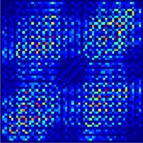
New J. Phys. 23 (2021) 065009                                                                                                 D Huber et al

   Figure 1. The figure illustrates the system of interest and the correspondence between three particles in a ring and a triangular
   billiard. Panel (a) Three particles in a ring. Two fermions have coordinates x1 and x2 , the coordinate of the impurity is y, see
   equation (1). Panel (b) The coordinates z1 and z2 describe the relative motion of three particles. Panel (c). The coordinates z and
   Z, which are obtained after rotation of z1 and z2 , see section 2 2. Panel (d) The triangular billiard is obtained upon rescaling the
   coordinates z and Z. To illustrate the transformation from (a) to (d), we sketch the (real-valued) ground-state wave function for
   κ = 1 in panels (b)–(d). The blue (red) color denotes negative (positive) values of ψ P=0 (see equation (5)), which is chosen to be
   real in our analysis. The intensity matches the absolute value. Note that in panel (d), we show only z̃ > 0. The wave function for
   z̃ < 0 is obtained from the fermionic symmetry by reflection on the Z̃ axis.

    The function ψ P is an eigenstate of the Hamiltonian
                                                           2      2
                                           1  ∂2        1  ∂           P ∂
                                              2                             2
                                    HP = −            −               +i           ,                                                   (6)
                                           2 i=1 ∂zi2   2κ i=1 ∂zi       κ i=1 ∂zi

which will be the cornerstone of our analysis. As we show below, it is enough to consider only HP=0 for our
                        H0, we resortto exact diagonalization
purposes. To diagonalize                                        in a suitable basis. As a basis element, we use
the real functions sin n1 Lπz1 sin n2 Lπz2 − sin n1Lπz2 sin n2Lπz1 , where n1 and n2 are integers with
nmax > n1 > n2 > 0, which is a standard choice for this type of problems, see, e.g., [51, 52]. Our choice of
the basis ensures that ψ P=0 is real for the ground and all excited states. The parameter nmax defines the
maximum element beyond which the basis is truncated. Note that the basis element is the eigenstate of the
system for 1/κ = 0. Therefore, we expect exact diagonalization to perform best for large values of κ and
more poorly for κ = 1. To estimate the accuracy of our results, we benchmark against the exact solution for
an equilateral triangle (κ = 1), see the discussion in the appendix. Using nmax = 130, we calculate about
4000 states whose energies have relative accuracy of the order of 10−3 . This set of 4000 states is an input for
our analysis in the next section.
    To summarize this subsection: we perform the transformation from H, φ to HP , ψ P to eliminate the
coordinate of the impurity from the consideration. Our procedure can be considered as the Lee–Low–Pines
transformation [53] in coordinate space, which is a known tool for studying many-body systems with
impurities in a ring [54–57]. Below we argue that HP can be further mapped onto a triangular billiard. Note
however that we are going to work with HP everywhere. Its eigenfunctions are defined on a square (see
figure 1(b)), allowing us to use them directly as an input for ConvNets.

2.2. Mapping onto a triangular billiard
It is known that three particles in a ring can be mapped onto a triangular billiard [39, 40]. Here we show
this mapping starting with HP . First of all we rotate the system of coordinates to eliminate the mixed√
derivative ∂z∂1 ∂z∂2 ; see figure 1(c). To this end, we introduce the system of coordinates z = (z2 − z1 )/ 2 and
                   √
Z = (z2 + z1 )/ 2, where the Hamiltonian reads as
                                                                             √
                                                 1 ∂2     1 ∂2     1 ∂2        2P ∂
                                   HP (z, Z) = −      2
                                                        −      2
                                                                 −      2
                                                                          +i        .                                                  (7)
                                                 2 ∂z     2 ∂Z     κ ∂Z       κ ∂Z

                                                        4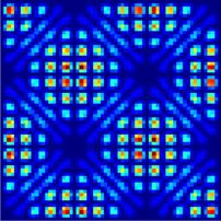
New J. Phys. 23 (2021) 065009                                                                        D Huber et al

                                                                           √
The last term here can be eliminated by a gauge transformation ψP → exp iκ+2P2 Z ψP . Therefore, in what
follows we only consider P = 0 without loss of generality. We shall omit the subscript, i.e., we write ψ. Note
that it is enough to study only z  0, because of the symmetry of the problem.
    To derive the standard Hamiltonian for quantum billiards:
                                                   1 ∂2      1 ∂2
                                            h=−          2
                                                           −          ,                                       (8)
                                                   2 ∂z̃     2 ∂ Z̃ 2
                                                                                √
we rescale and shift the coordinates as z̃ = z, and Z̃ = κ/(κ + 2)(Z − L/ 2), see figure 1(d). The
Hamiltonian h is defined on an isosceles triangle with the base angle obtained from tan(α) = (κ + 2)/κ.
For systems with more particles the corresponding transformations H → HP → h lead to quantum billiards
in polytopes, allowing one to connect an N-body quantum mechanical problem to a quantum billiard in
N − 1 dimensions. This can be a route for finding new applications of solvable models, see references
[39, 46, 48].
    Finally, we note that if the interaction term in equation (1) was an impenetrable wall with some radius R
instead of the delta function, then the considerations above would also lead to a mapping of the system
onto a triangle. (See reference [58] for an illustration with an equilateral triangle.)

3. Properties of the system

A discussion of highly excited states of triangular billiards can be found in the literature [22–26]. However,
we find it necessary to review some known results and calculate some new quantities in order to explain our
current understanding of the difference between integrable and non-integrable states. In principle, highly
excited states of a quantum system can be simulated using microwave resonators (see, e.g., [59, 60]), or
generated by means of Floquet engineering—by choosing the driving frequency to match the energy
difference between the initial and the desired final state (see, e.g., reference [61]). Therefore the results of
this section are not of purely theoretical interest, as they can be observed in a laboratory.
    As we outlined in the introduction, there are two main approaches for analyzing a connection between
highly-excited states and classical integrability. The first one relies on statistical properties of the energy
spectra, while the second one focuses on the morphology of individual quantum states. This section sets the
stage for our further study by discussing these approaches in more detail.

3.1. Energy
We start by calculating the energy spectrum. It provides a basic understanding of the evolution from an
‘integrable’ to a ‘chaotic’ system in our work as a function of κ. We present the first 30 states of H0 in
figure 2 (top). Note that an isosceles triangle has a symmetry axis (Z̃ → −Z̃), which corresponds to a mirror
transformation (in the particle picture this symmetry corresponds to zi → L − zi ). The wave function can
be symmetric or antisymmetric with respect to the mirror transformation and we consider these cases
separately. The former states are denoted as having p = 1, and the latter have p = −1.
    The energy spectrum features inflation of the spacing between levels, which can be understood as a
repulsion of levels in the Pechukas gas [62, 63]. According to Weyl’s law, it can also be interpreted as a
change of the density of states, ρ(κ) (E) = dN/dE, where N(E) is the number of states with the energy less
than E. The function ρ(κ) (E) can be easily calculated using Weyl’s law [64] for the triangular billiard
described by the Hamiltonian h:
                                                           L2      κ
                                          ρ(κ) (E → ∞) →              .                                    (9)
                                                           4π κ + 2
The density of states is independent of the energy in this equation because we work with a two-dimensional
object. Equation (9) is derived assuming large values of E, however, in practice, it also describes well the
density of states in a lower part of spectrum (cf reference [24]). If we multiply the energies presented in
figure 2 (top) by ρ(κ) then we obtain a spectrum without inflation, i.e., all levels are equally spaced on
average, see figure 2 (bottom).
    Multiplication of E by ρ(κ) is a simple example of unfolding, which allows us to directly compare
features of the energy spectrum for different values of κ. The goal of the unfolding is to extract the ‘average’
properties of the levels distribution and, thus, diminish the effect of local level density fluctuations in the
spectrum. While there are many possible ways to implement the unfolding procedure, which depend on the
properties of the energy spectrum (for further information see, e.g., references [9, 65, 66]), the ultimate goal
is to obtain rescaled levels with unit mean spacing. Below, we rescale all of the energy levels by the mean
distance between them, thus, obtaining the unit mean spacing. We benchmarked results of this unfolding
against more complicated approaches, and found qualitatively equivalent outcomes.

                                             5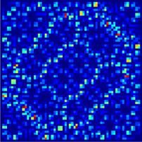
New J. Phys. 23 (2021) 065009                                                                                                D Huber et al

   Figure 2. The spectrum of the Hamiltonian HP from equation (7) as a function of the mass ratio, κ. The figure presents the first
   30 states: 15 mirror-symmetric states, p = 1, (red, solid curves), and 15 mirror-antisymmetric states, p = −1, (blue, dashed
   curves). The top panel shows the eigenstates of equation (6). The bottom panel shows these energies multipled by ρ(κ) from
   equation (9).

   Figure 3. The histogram shows the nearest-neighbor distribution, P(s), as a function of s for different values of the mass ratio, κ.
   The (red) solid curve shows the Wigner distribution from equation (10). The (black) dashed curve shows the Poisson
   distribution, e−s . To produce these figures, only states with p = 1 are used.

    We use unfolded spectra to analyze the distribution of nearest neighbors, P(s), which shows the
probability that the distances between a random pair of two neighboring energy levels is s. The function
P(s) is presented in figure 3, see also [24, 25, 45], where some limiting cases are analyzed. For the sake of
discussion, we only study the states with p = 1, however, we have checked that the case with p = −1 leads
to qualitatively identical results. The size of bins in the histograms in figure 3 is virtually arbitrary [66]. For
visual convenience, we have followed a rule of thumb that the number of bins should be taken at
approximately a square root of the number of the considered levels.
    Figure 3 shows a transition from regular to chaotic when the mass ratio changes from κ = 1 to larger
values. The degeneracies in the energy spectrum for κ = 1 and 1/κ = 0 lead to well spaced bins in the
figure. This behavior is however rather unique, and it is immediately broken for other mass ratios. For
example, already for κ = 1.2 the levels start to repel each other, and the distribution P(s) can be
approximated by the Wigner distribution [8]

                                                                      πs − πs2
                                                        PGOE (s) =      e 4 .                                                        (10)
                                                                      2

                                                        6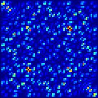
New J. Phys. 23 (2021) 065009                                                                                                D Huber et al

    Figure 4. The minimal distance between energy levels as a function of the number of considered levels. The data points are given
    as (red) crosses. The (black) solid curve is added to guide the eye. The left panels show δ min for κ = 5 and p = ±1. The right
    panels display δ min averaged over different
                                            √ mass ratios κ (see the text for details). The (green) dashed curves in the right panels
    show the best-fit to the asymptotic 1/ N behavior, which is expected for random matrices.

Note that it is important to use only one value of p for this conclusion. Levels that correspond to different
values of p do not repel each other, and the Wigner distribution cannot be realized [24].
    It is impossible to analyze every value of κ. However, we can also say something on average about our
system. To that end, we calculate the dependence of the minimal distance between levels as a function of the
number of considered levels, δmin (N) = inf En − En−1 n δ min is given by
   − πδmin
(1 √      2
            /4)N . To keep this probability independent of N, the parameter δ min must be proportional to
1/ N.
    We show δ min for our  √ system for κ = 5 in figure 4 (left panels). We see that for a given value of κ it is
impossible to verify 1/ N scaling, at least for the considered amount of eigenstates. However, the
randomness present in a mass-imbalanced system can be recovered. To show this, we average δ min over
                           average
different masses, i.e., δmin = M    1
                                          δmin (κi ), where M determines how many values of κ appear in the
sum. To produce figure 4 (right panels), we sum over the following      √ values of the mass ratios:
                                         average
κ = 1.1, 1.2, . . . , 5. The parameter δmin      has approximately 1/ N behavior at large values of N, which
confirms our expectation that systems with 1/κ ∈ (0, 1) are not integrable.

3.2. Wave function
The analysis above shows a drastic change of properties of the system when moving from integrable to
non-integrable regimes. Information about this transition is extracted by analyzing the energy levels as in
figure 3, although, the correspondence principle conjectures properties at the level of individual wave
functions. The wave function of a highly excited state contains too much information for the human eye,
and one has to rely on a few existing conjectures that allow one to connect classical chaos to quantum states.
For example, the chaotic states are expected to be similar to a random superposition of plane waves [6],
since the underlying classical phase space has no structure, i.e., the classical motion is not associated with
motion on a two-dimensional torus. This expectation applies to a typical random state (not to atypical, e.g.,
scared states [69]). In contrast, the wave functions of integrable states are expected to have some non-trivial
morphology, since classical phase space of integrable systems has some structure. Below, we illustrate these
ideas for our problem. We focus on a distribution of wave-function amplitudes, although, other signatures
of ‘chaos’ in eigenstates connected to local currents and nodal lines6 [70–72] will also be important when
we analyze our NN.

6 The dog-or-cat classifier in this case is a network with one output label for a dog and one for a cat, which has been trained using a set
of a few thousand pictures.

                                                        7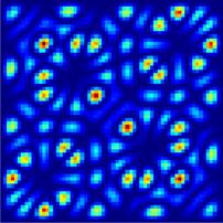
New J. Phys. 23 (2021) 065009                                                                                                D Huber et al

     Figure 5. The distributions of values of |ψ| for different mass ratios, κ = mI /m. The histogram describes the probability that a
     pixel has a value of |ψ| in a specific interval. For the main plots, we use a 315 × 315 pixel raster image of |ψ|. The insets are
     showing P(ψ) for the state represented by 33 × 33 pixel image. The (red) solid curve shows the prediction of equation (11) (no
     fit parameters).

  A celebrated result of the random-wave conjecture is a Gaussian distribution of wave-function
amplitudes, see examples in references [73–75]:

                                                                    1     |ψ|2
                                                                        −
                                                           P(ψ) = √    e 2v2 ,                                                           (11)
                                                                   2πv

where the variance v = 1/L fixes the normalization of the wave function7 . We present our numerical
calculations of P(ψ) in figure 5. For this figure, we discretize the wave function for the 500th state using
either a 315 × 315 pixel grid or a 33 × 33 pixel grid, and assign to each unit of the grid a value that
corresponds to ψ in the center of the unit. The distribution of these central values for a given value of κ is
presented as a histogram in figure 5. For κ = 1 the P(ψ) resembles an exponential function (cf reference
[75]). For larger values of κ, a Gaussian profile is developed. The distinction between the histogram and
equation (11) is clear for κ = 1. For 1/κ = 0 the difference is less evident. Note that the peak at ψ = 0 is
enhanced in comparison to the prediction of equation (11) for all values of κ. This is due to the
evanescence of the wave function at the boundaries, which is a finite-size effect beyond equation (11).
Finally, the characteristics of the states are also visible in a low-resolution images, see the insets of figure 5.
This feature will be used in the design of our NN discussed below.

4. Neural network

To construct a NN that can distinguish integrable states from non-integrable ones, we need to
(a) Prepare a data set for training the network
(b) Choose a suitable architecture and a training algorithm
      In this section, we discuss these two items in detail.

7   A nodal line is a set of points {X, Y} that satisfy ψ(X, Y) = 0.

                                                            8
New J. Phys. 23 (2021) 065009 D Huber et al
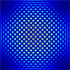
Figure 6. Schematic representations of a probability distribution of a state for 1/κ = 0 susceptible to aliasing. The left image
shows a high-resolution representation (320 × 320 pixel image). This representation contains too many pixels for our purposes,
and can be optimized. The right images present two low-resolution representations, which we use to train the network. The
representation with 33 × 33 pixels does not contain enough information and spatial aliasing occurs. The representation with
64 × 64 pixels contains all relevant information, and is used for the analysis in section 5.
4.1. A data set
As data set we use the set A made of two-dimensional images that represent highly excited states. We can
use images of (real) wave functions, ψ(z1 , z2 ) or probability densities, |ψ(z1 , z2 )|2 . We have checked that
these two representations lead to similar results. In the paper, we present only our findings for |ψ(z1 , z2 )|2 .
To produce A, we diagonalize the Hamiltonian HP=0 of equation (6) for κ = 1, 2, 5 and 1/κ = 0. Each
image has a label—integrable (for κ = 1 and 1/κ = 0) or non-integrable (for κ = 2 and 5)8 . We do not
include information about the mirror symmetry, i.e., states with different values of p are treated on the
same footing, since we do not expect that this information is relevant for a coarse-grained (see below)
image of |ψ(z1 , z2 )|2 . This allows us to work with twice as large datasets compared to figure (3). Each mass
ratio contributes 1000 states to A, which therefore contains 4000 images in total. It is reasonable to not use
data sets that contain states with very different energies: very different energies lead to very different length
scales, and hence different information content that should be learned. We choose to include all states from
the 50th to 1050th excited states. Not much should be deducible about the low-lying states (with N ∼ 10)
from the correspondence principle, therefore, we do not use them in our study.
A wave function ψ(z1 , z2 ) is a continuous function of the variables z1 and z2 , see figure 1(b). To use it as
an input for a network, we need to discretize and coarse-grain it. To this end, we represent ψ as a 64 × 64
pixel image, and as the value of the pixel we use the value of the wave function at the center of the pixel9 .
The resolution is important for this discretization. Low resolution might not be able to capture oscillations
present in highly excited states, leading to a loss of important physical√ information. For example, the
approximately Nth state in the spectrum√ for
√ 1/κ = 0 will have about N oscillations in each direction, and
it is important therefore to use a 2 N × 2 N representation of the wave function (similar to the
Nyquist–Shannon sampling theorem)10 . For a lower resolution, the oscillations are not faithfully
reproduced in the low resolution image and spatial aliasing occurs. We illustrate this using the 33 × 33
resolution in figure 6 for an integrable state that is susceptible to spatial aliasing.
Note that out of curiosity, we have also used images with 33 × 33 pixel resolution to train our network.
The network could reach relatively high accuracy (higher than 90%). However, not all integrable states were
detected properly. For example, the one in figure 6 was classified as non-integrable by the network. In
general, spatial aliasing is more damaging for integrable states, which have symmetries that should be
respected; non-integrable states are more random, and some noise does not change the classification of the
8 2 2
2 2
The
value of v is calculated by using the average valueof 2ψ , i.e., ψ = x P(x) dx, in the normalization condition, i.e., ψ dz1 dz2 =
2
ψ dz1 dz2 = 1, which leads to the condition on v as x P(x)dx = 1/ dz1 dz2 .
9 To avoid any bias toward non-integrable states, we use non-integrable states for only two values of κ. However, we have checked that
our conclusions hold also true if we include other values of κ into the data set, in particular, if we add 1000 states to A from a system
with κ = 15.
9New J. Phys. 23 (2021) 065009 D Huber et al
Figure 7. An illustration of the ConvNet used in our analysis. An input layer, 64 × 64 image, is followed by a sequence of layers:
a convolutional layer, a pooling layer, a convolutional layer, a pooling layer, and two fully connected layers. The last layer is used
to produce an output layer, which is made out of two neurons. In this NN, we use the rectified linear activation function (ReLU).
network. Everywhere below we use the 64 × 64 pixel representation, which gives a sufficiently accurate
representation of the state, so that we do not need to worry that the network learns unphysical properties.
Note that certain local features (e.g., ψ(z1 = z2 ) = 0) of the wave function may disappear at this resolution.
The overall high accuracy of our network suggests that such features are not important for our analysis.
The set A seems somewhat small. For example, the well-known Asirra dataset [76] for the cat–dog
classification contains 25 000 images that are commonly used to test and compare different image
recognition techniques. However, we will see that A is large enough to train a network that can accurately
classify integrable and non-integrable states. The dataset A is further divided into two parts. We draw
randomly 85% of all states and use them as a training set. The remaining 15% is used for testing. We fix the
random seed used for drawing to avoid discrepancies between different realizations of the network. It is
worthwhile noting that in image-recognition applications, the dataset A may be divided into more than two
parts. For example, in addition to the training set and testing set, one can introduce a validation (or
development) set [77], which is used to fine-tune parameters of the model. We do not use this additional
set here. The focus of this work is on understanding features of our general image classificator, and not on
improving its accuracy.
4.2. Architecture
The NN in our problem is a map that acts in the space X made of all 64 × 64 pixel representations of |ψ|2 .
By analogy to the standard dog-vs-cat classifier, the output of the network is a vector with two elements b.
Note that n output neurons are usual for classifying n classes. However, it is possible to use a single output
neuron for a binary classification, since we know that b1 + b2 must be equal to one. We use two neurons,
since such an architecture can be straightforwardly extended to more output neurons, which may be useful
for the future studies, as we discuss in section 6.
The first element of the output layer, 0 b1 1, determines the probability that the input state is
integrable, whereas the second element b2 = 1 − b1 is the probability that the input state is non-integrable.
An input state is classified as integrable (non-integrable) if b1 > b2 (b1 < b2 ).
Mathematically, the network is a map f, which acts on the element a of X as
f(a; θ, θhyp ) = b. (12)
The f is determined by the set of parameters θ, which are optimized by training. Since our problem is
similar to image recognition (in particular dog-vs-cat classification) [10], which is one of the standard
applications in machine learning, we can use the already known training routines (SGD, ADAM,
Adadelta,. . . ) for optimizing θ. The outcome for the parameters θ may vary between different trainings, and
we use this variability to check the universality of our results. Specifications of f that are not trained but
specified by the user are called hyperparameters (θhyp ). Examples of them include the loss function,
optimization algorithm, learning rate, network architecture, size of batches that the data is split into for
training (batch size) and the length of training (epochs). We find hyperparameters by trial-and-error.
The simplest form of a network is called a dense network in which all input neurons are connected to all
output neurons. However in most cases of image detection, this architecture does not lead to accurate
results. This also happens in our case. Instead, we resort to a standard architecture based on ConvNets for
image recognition, see figure 710 . Our network consists of two convolutional layers and two max-pooling
10The color depth (i.e., how many colors are available) of a pixel is effectively given by the numerical precision used to produce the
input data. If experimental data is used as an input, then their accuracy will determine the color depth of a pixel.
10New J. Phys. 23 (2021) 065009 D Huber et al
layers. The former use a set of filters and apply them in parts to the image to produce a new smaller image.
This is somewhat analogous to a renormalization group transformation [78]. A set of images that are
produced by a convolutional layer is called feature map. Each convolutional layer is followed by a
max-pooling layer which reduces the size of an image. The size of max-pooling layers is a hyperparameter.
In our implementation, max-pooling layers take the largest pixel out of groups of 2 by 2.
One could use architectures different from the one presented in figure 7. However, we checked that they
do not lead to noticeably different results. Therefore, we do not investigate this possibility further.
5. Numerical experiments
Following the discussion in section 4, we train and test the NN. We observe that a typical accuracy of the
trained network (which we refer later to as N ) is ∼ 97%11 . This means that about 18 states out of 600 used
for testing are given the wrong label. Out of these 18 states, roughly one half is integrable. We illustrate
typical wave functions that are classified correctly and wrongly in figure 8. It does not mean that these states
are in anyway special—another implementation (e.g., another random seed for weights) will lead to other
states that are given the wrong label. Non-integrable states with some structure (e.g., states with scars) in
general confuse the network and might be classified as integrable.
In general, it is hard to interpret predictions of the NN. This becomes clear after noticing that some
images can be changed so that a human eye can hardly detect any variation. At the same time, this change
completely modifies the prediction of the network. Such a change can be accomplished especially easily for
integrable states12 , thus, DL confirms our intuition that integrable states are a small subset in the space of all
possible states. However, such a situation can also occur for non-integrable (in particular scared) states. We
illustrate this in figure 9, which is obtained by slightly modifying states from A using tools of adversarial
machine learning, see reference [79].
One simple way to extract features of the network is to look at feature maps, which should contain
information about what features are important. For example, the first layer might represent edges at
particular parts of the image, the second might detect specific arrangements of edges, etc. However, we
could not extract any meaningful information from this analysis. This is expected: the features of integrable
and non-integrable states are more abstract and not as intuitive as the features of cats and dogs or images of
other objects we encounter in everyday life.
Other approaches to analyze a network rely on estimating the effect of removing a single (or a group) of
elements on a model. For large data sets, this can be done by introducing influence functions [80, 81]. Here,
we work with a small data set, and, therefore, we can calculate directly the actual effect of leaving states out
of training on a given prediction. Our goal is to understand correlations between states of different energies.
In our implementation we compare the prediction of f from equation (12) for |ψ|2 to a prediction of f−β for
the same state. Here f−β is obtained by training a NN after leaving out the set β from A. The comparison of
the two predictions (f − f−β ) allows us to estimate the importance of the set β for the classification of a test
state ψ 13 . We present a typical example in figure 10, where one observes no clear energy correlations, which
suggests that the network learns different energies simultaneously, at least in the energy interval we choose
to work with. This observation is consistent with our discussion below that the network does not learn
specific features of non-integrable states, and only overall randomness, which does not depend on a specific
energy window. Finally, we note that our result in figure 10 is an example of cross-validation. It suggests
weak dependence of the output of the network on a particular state, which is a necessary condition for a
good performance of our NN.
Below, we explore the network N further. To this end, we resort to numerical experiments. We employ
N to analyze states outside of the set A. First, we study physical states, and then non-physical ones.
5.1. Classification of physical states outside of A
As a first application of N , we use it to classify eigen-states of HP=0 not used in the training, i.e., for
κ = 1, 2, 5 and 1/κ = 0. These states are non-integrable (cf figure 4), and we observe that N accurately
classifies them as such as long as κ is far enough from κ = 1, see figure 11. The figure shows that
11 We use the word ‘typical’ to emphasize that a trained network depends on hyperparameters and random seeds. Even for a given set of
hyperparameters, each set of random parameters leads to a slightly different network N . We can tune hyperparameters to reach higher
accuracies. We do not discuss this possibility here, since high accuracy is not the main purpose of our study.
12 Tools of adversarial machine learning can make a NN classify an arbitrary integrable state as ‘non-integrable’ using a small number
(∼ 100) of iterations. This is not possible for an arbitrary non-integrable state.
13 Note that it is important to choose a test state ψ for which the network gives an accurate prediction with high confidence level, i.e.,
bi → 1. For other states, an intrinsic randomness of ConvNets can lead to a drastic change in the classification of the network.
11New J. Phys. 23 (2021) 065009 D Huber et al
Figure 8. The figure shows |ψ|2 of exemplary integrable (upper row) and non-integrable states (lower row) together with the
corresponding prediction of the network. The network assigns a wrong (correct) label for the states in the first (second) column.
The third column shows states, which are identified correctly by the network, but with a low confidence level (with about 60%).
In other words, the states in the third column confuse the network and lead to b1 b2 in equation (12).
Figure 9. Fooling the network. The first column shows |ψ|2 of the initial state, which is correctly identified by the network as
integrable (non-integrable) in the upper (lower) panel. The second column shows a slightly modified image of |ψ|2 , which is
wrongly identified by the network. The third column shows the difference between the first and second columns divided by the
maximum value of the initial state. The color chart corresponds to the images in the third graph only.
predictions of N are not accurate only for systems with κ = 1 + , where is a small parameter. These
systems are non-integrable, however, the morphology of their eigenstates is very similar to the integrable
ones at κ = 1. The network classifies them wrongly because of this. Already for κ 1.5, the accuracy of the
network is close to one, and it stays high for larger values of κ. The region between 1 and 1.5 can be
interpreted as a transition of the network classification from integrable to chaotic [13]. We do not expect
this region to be universal—it should depend on hyperparameters, and the states used for training of N .
Therefore, we do not investigate it further.
To test the network on integrable states, we use wave functions of two non-interacting bosons in a box
potential of size L:
Nk ,k
ΨB = 1 2 [sin(k1 z1 ) sin(k2 z2 ) + sin(k2 z1 ) sin(k1 z2 )] , (13)
L
√
where k1 k2 , and Nk1 ,k2 is a normalization constant, Nk1 =k2 = 1 and Nk1New J. Phys. 23 (2021) 065009 D Huber et al
Figure 10. A typical outcome of a leave-one-out algorithm. (Top) The panel shows f1 − f1,−β for β that consists of a single state
as a function of the energy of the state that was left out. (Bottom) The panel shows f1 − f1,−β for β that consists of ten consecutive
states as a function of the energy of the first state in β. The test state, ψ, here is for κ = 5, its energy is 534.86 (in our units).
Figure 11. Accuracy of the network N as a function of the mass imbalance κ. The shaded area shows the uncertainty area. To
obtain it, we train a set of NNs using different random seeds. The highest (lowest) accuracy from a set produces an upper (lower)
bound of the uncertainty area. The dots are calculated, and the curves are added to guide the eye. The points κ = 1, 2, 5, which
are used for training, are shown with vertical lines. The point κ = 1 corresponds to an integrable system. All other points of the
x-axis are expected to be non-integrable (cf figure 3).
from the mapping discussed for fermions (see figure 1) assuming that the impurity is infinitely heavy. In
particular, figure 1(b) shows the geometry of the problem in this case. Note that the bosonic symmetry
requires that the derivative of the wave function vanishes on the diagonal of the square in figure 1(b). The
high accuracy of the classification of the bosonic states suggests that a network trained using the Dirichlet
boundary condition can also be used to classify states with the Neumann boundary condition. In other
words, the network is mainly concerned with the ‘bulk’ properties of the wave function, the boundary is not
important.
5.2. Classification of non-physical states
The network N can classify any 64 × 64 pixel input image, and it is interesting to explore the outcome of
the network for images that have no direct physical meaning. We start by considering non-normalized
eigenstates of HP=0 . The normalization coefficient does not change the physics behind the states. However,
since the function f is non-linear, i.e., f(αx) = αf(x), input states must have the same normalization as the
states in the training set for a meaningful interpretation of the network. To illustrate this statement, we use
states from A multiplied by a factor, i.e., we use α|ψ|2 instead of |ψ|2 . Figure 12 shows the accuracy14 of the
14 Here we still can talk about the accuracy, since the states αψ 2 correspond to integrable or non-integrable situations.
13New J. Phys. 23 (2021) 065009 D Huber et al
Figure 12. Prediction of the network for the states from A multiplied by a factor α. The curves show the accuracies for four
values of the mass ratio κ. The average of these four curves is shown as a thick solid curve.
Figure 13. Predictions of the network for the states from A with noise. The (red) dashed curve shows the accuracy for states
which are integrable for σ = 0 (the accuracy here is defined as the percentage of the states identified as integrable). The (green)
dotted curve shows the accuracy of the network for non-integrable states. The (blue) solid curve shows the average of the first
two curves.
network as a function of α. The maximum accuracy of the network is reached at α = 1, i.e., for the states
used for the training. Integrable states are classified as non-integrable almost everywhere except close to
α = 1. A different situation happens for non-integrable states. They are classified correctly almost
everywhere, and we conclude that they are less susceptible to the factor α. The shape of the curves in
figure 12 is not universal, it depends on hyperparameters of the network. However, a general conclusion
holds—the normalization is important, and we use normalized input functions in the further analysis. In
principle, it is possible to reduce the sensitivity of our NN to α. To that end, one needs to add states α|ψ|2
to a training set (see data augmentation in DL [82]). We do not pursue this possibility here, to demonstrate
that the sensitivity of integrable states on α is different from that for non-integrable states.
As a next step, we add noise to the images from A, i.e., we build a new data set using wave functions
ψ̃ = aσ ψ(1 + rσ ), where rσ is a noise function whose values are drawn from the normal distribution with
zero mean and the standard deviation σ; aσ is a normalization factor, which is determined for each input
state depending on the function rσ . We assume that rσ possesses basic symmetries of the problem: fermionic
and mirror. Functions ψ̃ naturally appear in applications, and therefore, it is interesting to investigate the
resilience of the network to random noise. We use 4000 states of A with noise to make a relevant statistical
statement, see figure 13. Small values of σ lead to weak noise and the network correctly classifies almost all
input states. However, larger values of σ lead to confusing input states, and the network fails. It actually fails
for integrable states where the noise destroys correlations. The accuracy for non-integrable states is always
high. The resilience of the network to noise suggests it as a tool to analyze experimental data (e.g., obtained
using microwave billiards). These experiments [21] can produce a large amount of data, however, there are
limited variety of tools to analyze the simulated states. In particular, NNs can be used to identify atypical
states, which do not fit the overall pattern, e.g., scars.
Our choice of ψ̃ to represent a noisy state is not unique. One could, for example, use instead of ψ̃ the
function ψ̄ = aσ (ψ + Grσ ), where the parameter G determines the relative weight of the function rσ , which
is defined as above. Note that G cannot be absorbed in rσ , since for a given value of σ, the average
14New J. Phys. 23 (2021) 065009 D Huber et al
Figure 14. The histogram shows distributions of probability-density amplitudes for different values of the mass ratio, κ. We use
a 315 × 315 pixel representation of the probability density, |ψ|2 , for this analysis. The insets give P(|ψ|2 ) for the probability
density at the lower (33 × 33) pixel resolution.
amplitude of rσ2 is well defined. For G = 0, the function ψ̄ is a physical state, whereas for G → ∞, the
function ψ̄ is completely random. In contrast to ψ̃, the function ψ̄ can become completely independent of
the function ψ. This happens if the parameter G is large.
For the data set based upon ψ̄ with small values of G, the accuracy of the network is similar to that
presented in figure 13. For large values of G, the network is confused and classifies states in a random
manner. This behavior should be compared with the data set ψ̃ for which the states are classified as
non-integrable when the noise is large. To understand this difference, note that ψ̃ retains information about
the nodal lines of the physical state. It turns out that it is important for the input state to have enough pixels
with small (zero) values (note that the number of zero pixels is very large for |ψ|2 , see figure 14). Only such
states have a direct meaning for the network, all other states confuse the network and do not allow for
extraction of any meaningful information. It is worthwhile noting that the network does not learn the
physical nodal lines. We checked that almost any random state with a large number ( 30%–40%) of zero
pixels is classified as non-integrable.
Our discussion above suggests that the network classifies all states with nodal lines but without clear
spatial correlations as non-integrable. In other words, the network perceives almost all states as
non-integrable, and there are only a few islands recognized as integrable states. Such asymmetry of learning
is not expected to happen for labels with equal significance (cat and dog for example). We speculate that the
observed asymmetry is related to the fact that non-integrable states that correspond to different energies do
not correlate in space [83], and, therefore, a NN cannot learn any significant patterns when trained with
those states.
All in all, the state classificator validates our expectation that non-integrable states are random and
abundant, whereas integrable states are rather unique and occur rarely. For example, in our analysis,
integrable states are a set of measure zero in κ, and perturbation in κ or noise change the prediction of N
for these states. The asymmetry also suggests that the standard implementation of DL presented here should
be modified to reveal the physics behind non-integrable states. The present network does not distinguish a
non-physical random state with a large number of zero values from a physical non-integrable state since it
was not trained for that question. A possible modification is the addition of an extra label (b3 in
equation (12)) for non-physical states. Since there are many possible non-physical states, one should frame
the problem having an experimental or numerical set-up in mind, where such states have some origin and
interpretation. We leave an investigation of this possibility for future studies.
15New J. Phys. 23 (2021) 065009 D Huber et al
Finally, we note that the conclusion that the network classifies almost all random images as
non-integrable is general—it does not depend on the values of hyperparameters, initial seed or the
distribution (Laplace, Gaussian, etc) that we use for generation of the random states. We check this by
performing a number of numerical experiments. In particular, this means that the network does not learn
P(ψ) from equation (11).
To summarize: a trained network can accurately classify integrable and non-integrable states. The
network can even classify input states from an orthogonal (bosonic) Hilbert space, on which it can have no
microscopic information. Thus network identifies generic features of the ‘integrable’ and ‘non-integrable’
states, although this might be not that surprising provided that we work with low-resolution 64 × 64 pixel
images. The network classifies almost all random images with nodal lines as non-integrable, which suggests
that useful information for the network is mostly contained in integrable states.
6. Summary and outlook
We used convolutional NNs to analyze states of a quantum triangular billiard illustrated in figure 1. We
argued that NNs can correctly classify integrable and non-integrable states. The important features of the
states for the network are the normalization of the wave functions and a large number of zero elements,
corresponding to the existence of a nodal line. Almost any random image that satisfies these criteria is
classified as non-integrable. All in all, the NN supports our expectation that non-integrable states are
resilient to noise as discussed in subsection 5.2, and have a ‘random’ structure, unlike integrable states
whose structure can be revealed by considering, for example, nodal lines.
Our results suggest that machine learning tools can be used to analyze the morphology of wave
functions of highly excited states obtained numerically or experimentally, to solve problems like: find
exceptional states (e.g., scars or integrable states) in the spectra, investigate the transition from chaotic to
integrable dynamics, etc. However, further investigations are needed to set the limits of applicability for DL
tools. For example, our network considers all states without clear correlations as non-integrable. This means
that it must be modified for the analysis of noisy data, where a noisy image without any physical meaning
could be classified as non-integrable. To circumvent this, one could introduce additional labels for training
the network. For example, one could consider three classes—‘integrable’, ‘non-integrable’, and ‘noise’. This
classification might allow for a more precise description of data sets, and may help one to extract more
information about the physics behind the problem.
We speculate that a network memorizes integrable states, and all other states are classified as
non-integrable, provided that an image has a large number of vanishing values. This would explain our
findings and it would align nicely with the observation that we observe no overfitting even after many
epochs of working through the training set. In the future, it will be interesting to use other integrable
systems to test this idea. In particular, one could use non-triangular billiards, or systems without an
impenetrable boundary. For example, one can consider a two-dimensional harmonic oscillator with cold
atoms. At a single body level, the integrability in this system can be broken by potential bumps [84, 85] or
spin–orbit coupling [86].
In the present work, we focus on data related to the spatial representation of quantum states. However,
our approach can also be used to analyze other data. For example, for few-body cold atom systems,
correlation functions in momentum space are of interest in theory and experiment (see, e.g., [87]).
Therefore, in the future, it will be interesting to train NNs using experimental/numerical data that
correspond to a momentum-space representation of quantum states, and study the corresponding features
of ‘quantum chaos’. Although, in the present work we focused on two-dimensional data (images of
probability densities), it might be interesting to consider higher-dimensional analogues (e.g., four-body
systems) as well. Further applications include the identification of phase transitions, the representation of
quantum many-body states, and the solution of many-body problems [88]. Thus machine learning
techniques may not only be used to classify quantum states but also to obtain them by solving the
corresponding many-body problem.
To extract further information about the map f, one could investigate its geometry close to its maximum
(minimum) values. For example, in the vicinity of some accurately determined integrable state (f1 (x0 ) = 1),
we can write
1
f1 (x0 + δx) 1 + δxT Gδx, (14)
2
where the position of the maximum x0 is understood as a vector and G is the Hessian matrix. The first
derivative of f1 vanishes since the function f1 is analytic and bounded. Eigenstates of the Hessian G provide
us with the most important correlations. A preliminary study shows that there are only a handful of
eigenvalues of G for our network, which suggests the next step in the analysis of our image classifier.
16You can also read