A portable lightweight in situ analysis (LISA) box for ice and snow analysis
←
→
Page content transcription
If your browser does not render page correctly, please read the page content below
The Cryosphere, 15, 3719–3730, 2021
https://doi.org/10.5194/tc-15-3719-2021
© Author(s) 2021. This work is distributed under
the Creative Commons Attribution 4.0 License.

A portable lightweight in situ analysis (LISA) box for ice
and snow analysis
Helle Astrid Kjær1 , Lisa Lolk Hauge1 , Marius Simonsen1 , Zurine Yoldi1 , Iben Koldtoft1 , Maria Hörhold2 ,
Johannes Freitag2 , Sepp Kipfstuhl1,2 , Anders Svensson1 , and Paul Vallelonga1,3
1 Physics
       of Ice, Climate and Earth (PICE), Niels Bohr Institute, University of Copenhagen, Copenhagen, Denmark
2 Alfred-Wegener-Institut,
                         Helmholtz-Zentrum für Polar- und Meeresforschung, Bremerhaven, Germany
3 UWA Oceans Institute, The University of Western Australia, Crawley, WA, Australia

Correspondence: Helle Astrid Kjær (hellek@fys.ku.dk)

Received: 10 February 2021 – Discussion started: 2 March 2021
Revised: 1 June 2021 – Accepted: 10 June 2021 – Published: 11 August 2021

Abstract. There are enormous costs involved in transport-         ing the change in SMB are made based on advanced ice
ing snow and ice samples to home laboratories for “simple”        sheet models, but they also rely on accurate accumulation es-
analyses in order to constrain annual layer thicknesses and       timates from past periods (Montgomery et al., 2018). Accu-
identify accumulation rates of specific sites. It is well known   mulation of the past can be reconstructed by means of ice and
that depositional noise, incurred from factors such as wind       firn core analysis. To estimate ice core ages, chemical profiles
drifts, seasonally biased deposition and melt layers can in-      are often used to generate annually resolved timescales (Win-
fluence individual snow and firn records and that multiple        strup et al., 2012; Svensson et al., 2008). However, ice cores
cores are required to produce statistically robust time series.   are spatially limited for practical reasons: drilling campaigns
Thus, at many sites, core samples are measured in the field       of deep ice cores are expensive, as they require the mainte-
for densification, but the annual accumulation and the con-       nance of large-scale facilities for several years; drilling cam-
tent of chemical impurities are often represented by just one     paigns of shorter snow and firn cores are cheaper, although
core to reduce transport costs. We have developed a portable      they are still costly in terms of time and money.
“lightweight in situ analysis” (LISA) box for ice, firn and           Having retrieved such snow/firn cores, annual layers and
snow analysis that is capable of constraining annual layers       accumulation rates can be directly reconstructed by inves-
through the continuous flow analysis of meltwater conduc-         tigating the chemical impurities within the ice. Several of
tivity and hydrogen peroxide under field conditions. The box      these impurities have annual cycles in Greenland snow and
can run using a small gasoline generator and weighs less than     ice – for example, insoluble dust particles and calcium peak
50 kg. The LISA box was tested under field conditions at the      in early spring as a result of increased storm activity, acids
East Greenland Ice-core Project (EastGRIP) deep ice core          peak in spring time following the Arctic haze phenomenon
drilling site in northern Greenland. Analysis of the top 2 m      and higher signals are observed with acid from volcanic erup-
of snow from seven sites in northern Greenland allowed the        tions, and hydrogen peroxide is driven by light processes
reconstruction of regional snow accumulation patterns for the     and peaks in midsummer (Gfeller et al., 2014; Legrand and
2015–2018 period (summer to summer).                              Mayewski, 1997). Using one or more profiles of an ice core
                                                                  site, an accurate timescale can be established by dating and,
                                                                  if the density is also measured, the local accumulation rate of
                                                                  a site can be reconstructed (Winstrup et al., 2019; Philippe et
1   Introduction                                                  al., 2016).
                                                                      The chemical profiles in ice cores can be obtained by
To evaluate future sea level changes, surface mass balance        means of continuous flow analysis (CFA), a fast way to ob-
(SMB) determinations of the major ice sheets and ice caps         tain high-resolution chemical profiles, performed in home
are an important constraint. Theoretical predictions regard-

Published by Copernicus Publications on behalf of the European Geosciences Union.
3720 H. A. Kjær et al.: Lightweight in situ analysis (LISA) box for ice and snow analysis
laboratories (Kaufmann et al., 2008; Bigler et al., 2011; Dall-
mayr et al., 2016). A generic CFA consists of a melt head,
which splits the sample stream into an inner uncontaminated
line and an outer possibly contaminated line. The inner line is
then split further, allowing a small amount of sample water
for each analytical measurement. Field campaigns with in-
camp melting and CFA are not carried out on a routine basis,
as the analytical set-ups require space, time and warm lab-
oratories on-site (Schüpbach et al., 2018). Thus, these cam-
paigns are limited to larger ice core drilling stations in Green-
land (NEEM community members et al., 2013) and Antarc-
tica where heavy and delicate instruments can be flown in
and out by large cargo aircraft, and warm buildings or areas
exists with space enough to construct a laboratory.
Here, we have developed a truly field-portable CFA set-
up that can determine annual layers in snow and firn. We
developed a system that is optimized for deep field deploy-
ment, which can be powered by a small gasoline generator
and operated in below-zero conditions. In addition, we made
it lightweight enough to be transported in the field by two
people. As time in the deep field is often limited, we also
aimed for a device that provides results quickly (so that the
spatial variability at a site can be investigated within a day
of field work) as well as an instrument that can be used by
laypeople.
In the summers of 2017 and 2019, we demonstrated the
LISA box under Greenland field conditions at the East
Greenland Ice-core Project (EastGRIP) ice core drilling site
(see map Fig. 1) by reconstructing accumulation from snow
cores covering the top 2 m of snowpack. Although the LISA
box may be used to melt ice cores, we will focus on the ap-
plication to snow and firn.
2 Materials and methods
The LISA box is a small CFA system set up to melt snow, firn Figure 1. Position of the sites studied using the LISA box (trian-
and ice cores and to analyse the meltwater for conductivity gles). The asterisks indicate deep ice core drilling sites. Note that
and hydrogen peroxide. two sites (S5 and S7) were investigated at EastGRIP. The back-
Overall, it consists of a square foam box with a lid ground altitude map of Greenland is based on the SeaRISE dataset
that provides insulation against external conditions. The (Bamber, 2001; Bamber et al., 2001).
outer dimensions of the box are 0.585 m (height) × 0.475 m
(width) × 0.765 m (length). The foam is 10 cm thick, mak-
ing the respective inner dimensions 0.35 m × 0.35 × 0.58 m. 2.1 Melt head and melt speed registration
A circular melt head is placed in the lid; inside the box, which
The melt head (shown as “A” in Fig. 2 and outlined in Fig. S2
is temperature controlled, a small version of a CFA system is
in the Supplement), which is used to melt the snow, firn or ice
set up, including a miniature computer for instrument control
sample, is placed in the lid of the foam box and reaches both
and storage (see Fig. 2).
the inner and outer side of the foam box with the intention
Some additional components are required outside the
that the sample is melted on the outside while meltwater is
LISA box: a handheld generator for power, a wastewater con-
transported into the box for further analysis.
tainer and pump, and a screen and keyboard for easy instru-
The melt head is circular to allow for the analysis of full-
ment adjustments. The LISA box is presented in more detail
sized snow and ice cores to avoid time-consuming cutting
in the following.
in the field. The melt head has an inclined surface to divert
the outer part of the melted core to waste as well as an in-
ner inclined conical surface for the collection of the sample
The Cryosphere, 15, 3719–3730, 2021 https://doi.org/10.5194/tc-15-3719-2021H. A. Kjær et al.: Lightweight in situ analysis (LISA) box for ice and snow analysis 3721
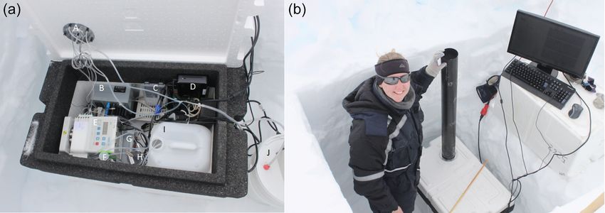
Figure 2. (a) An inside look at the LISA box. The letters in panel (a) denote the following: A – the underside of the melt head; B – the melt
head temperature regulator; C – the temperature proportional integral derivative (PID) that stabilizes the inner temperature of the box; D –
the computer; E – the peristaltic pump; F – the debubbler; G – the fluorescence box (F-box); H – the conductivity meter; I – the chemical
wastewater container; and J – a container for collecting waste water from the outer section of the melt head, which is located outside the
LISA box. (b) LISA box during field work 2017. The snow is collected in the black liner and melted continuously, while data can be observed
online on the attached screen.
meltwater (Fig. S3). The inclination prevents bubbles from ply registered by simultaneously determining the amount of
entering the sample line, as the conical shape melts the dif- core left above the melt head with a ruler and the time. While
ferent depths of the firn core at the same time and “floods” this method is clearly imprecise compared with the more ad-
the lower part of the inner cone. The volume of the inner cone vanced options that exist, it is also the simplest, as no com-
determines how much mixing happens in the sample stream plicated electronics are necessary, only a ruler, chronometer
before it is distributed to the analysis unit. As is done for all and a notebook, thereby reducing the weight requirements.
CFA systems to prevent contamination, the inner melt head
cone melts more water for the outer part of the core than is 2.2 Temperature stabilizer of inner box
being drained, thereby producing an overflow of inner melt-
water out toward the waste drainage. When aiming to move a CFA to the field, it is crucial to en-
The melt head is heated by heat cartridges (HHP30, Mick- sure a stable temperature environment for the measurement
enhagen GmbH, Lüdenscheid, Germany), which are con- apparatus and chemicals inside the box. Thus, a custom-built
trolled by a proportional integral derivative (PID, CN7532, thermostat is installed inside the LISA box to ensure a stable
Omega Engineering) device (“B” in Fig. 2; Fig. S1). One of temperature (inside the box) of between 17 and 18 ◦ C (“C”
the heat cartridges has an inbuilt J-type thermocouple that in Fig. 2). The thermostat and its digital display are mounted
provides the temperature for the PID, so that the tempera- on a stainless-steel plate that is fixed on the box wall. The
ture of the melt head can be regulated to obtain an optimum thermostat is connected to 200 W compact fan heater (FCH-
melt speed. The optimum melt speed is site dependent and FGC1 series, Omega Engineering) that sits at the bottom of
can, thus, be varied with the density of the sample and the the LISA box and is guarded by a fence to avoid contact with
expected annual layer thickness. the other box contents. The fan is always active to ensure that
The melt head (inner diameter of 11 cm to fit a 10 cm snow air is well mixed within the box and to distribute heat when
core) is made of solid aluminium, which was chosen for its required.
low density, high thermal conductivity and excellent corro-
2.3 Computer and communication devices
sion resistance. The inner cone is 7 cm higher than the deep-
est point of the melt head, which is 6 cm lower than the outer To control the measurement devices, the melt head tempera-
rim. There is one drainage hole in the centre of the melt ture and to save data, a miniature computer is mounted on the
head and five outer drainage holes. The inner cone volume wall of the box (Fig. 2-D); it is connected to a USB hub and
is 3.8 cm3 . Additional specifications of the melt head can be a RS232-to-USB converter (Digi International) that are also
found in Table S1 in the Supplement. inside the box as well as to a screen and keyboard outside the
The melt speed is a crucial parameter to obtain, as it is box.
used to reconstruct the depth of the analysed sample. Sev- The wires for the mouse and keyboard positioned outside
eral ways exists to determine melt speed in CFA systems, the box are connected via a small triangle cut in the side of
including encoders, lasers and image recognition (Bigler et the LISA box, as is the screen cable. The screen is connected
al., 2011; Dallmayr et al., 2016; McConnell et al., 2002). via a series of adapters (VGA–HDMI and HDMI–HDMI).
The melt speed in the portable CFA developed here is sim-
https://doi.org/10.5194/tc-15-3719-2021 The Cryosphere, 15, 3719–3730, 20213722 H. A. Kjær et al.: Lightweight in situ analysis (LISA) box for ice and snow analysis
of the debubbler. It is pumped at a speed of 1 mL min−1 (or
2 mL min−1 , depending on set-up) to be collected for further
analysis. As in all CFA systems, flow rates can be adjusted
depending on the requirements and the number of analysis
systems connected downstream.
2.4.2 Conductivity meter
The water is led from the debubbler to an Amber Science
3082 conductivity meter (“H” in Fig. 2 and “C” in Fig. 3)
(Bigler et al., 2011). The response time (5 %–95 % of signal)
Figure 3. The continuous flow analysis (CFA) set-up for the LISA of the instrument itself is just 3 s. However, the typical mea-
box. The frozen sample is melted on the melt head (M), and the surement resolution is only on the order of 20 s as a result of
meltwater is split into an inner uncontaminated sample line (I) and upstream smoothing in the debubbler and melt head.
an outer possibly contaminated line (O). The outer line is collected
in a waste bucket outside the box (WO). The inner line is pumped 2.4.3 Fluorescence measurements – H2 O2
to a debubbler (D), which is kept at a fixed volume by an overflow
line. From the debubbler, the sample reaches the conductivity me-
From the conductivity meter, the sample is mixed with a
tre (C) after which it is mixed with reagent (R) prior to analysis
reagent and measured by means of fluorescence. A custom
by fluorescence (F). The mixed water is then collected in a waste
bucket (W). Active pumping is illustrated using pentagons, and the box was built for fluorescence analysis in order to limit the
numbers within the pentagons indicate the flow rate in millilitres space used within the LISA box (F-box; “G” in Fig. 2 and
per minute (mL min−1 ). “F” in Fig. 3). The F-box allows for the determination of
two chemical species by means of fluorescence and is pow-
ered by a 5 V power supply. The two fluorescence systems in
The program that runs the CFA inside the LISA box is a the F-box can be independently activated or deactivated us-
custom-built LabVIEW program with an interface showing ing two switches at the front of the F-box. Serial connectors
the measurements in real time; thus, a first assessment of the and RS232 communication protocols were adopted to ensure
data can be done while in the field, allowing for an initial stability when moving the box between sites in the field.
data quality assessment during measurement. Inside the F-box, each of the two analytical lines consist
of a 10 mm path length cuvette (176.766-QS, Hellma) and a
2.4 Continuous flow scheme photomultiplier tube (PMT 9111, Sens-Tech, UK) in a light-
tight aluminium holder with a specific optical filter in front,
The overall CFA set-up for the LISA box is shown in Fig. 3 depending on the desired frequency of outgoing light (Bigler
and builds on conventional CFA instruments used for the et al., 2011).
analysis of ice cores using PEEK (polyether ether ketone) In the field, we only tested the F-box for the determination
connectors and PFA (perfluoroalkoxy) (1.55 mm inner di- of hydrogen peroxide (H2 O2 ), which is known to show clear
ameter, 1/8 inch outer diameter, IDEX) tubing (Bigler et annual signals in Greenland snow (Sigg and Neftel, 1988;
al., 2011; Kaufmann et al., 2008). Frey et al., 2006). The reagent is kept in a bottle at the bottom
of the LISA box and is added to the meltwater sample at a
2.4.1 Debubbler rate of 0.14 mL min−1 . The response time (5 %–95 % of sig-
nal) of the hydrogen peroxide system is just 13 s if fully opti-
An Ismatec IPC eight-channel peristaltic pump and Tygon mized (Röthlisberger et al., 2000); however, in a similar fash-
pump tubing are used for the inner line sample transport ion to the conductivity, it is influenced by upstream smooth-
through the CFA. A debubbler (see “F” in Fig. 2 and “D” in ing, and the resulting response is on the order of ∼ 40 s. A
Fig. 3) is implemented early in the system to ensure that po- 335 nm LED was used to excite the sample, and detection
tential air pumped into the system or short pauses in melting was carried out at 400 nm. The H2 O2 reagent consists of 1 L
do not interfere with the measurements downstream. The de- of purified water, 0.61 g of 4-ethylphenol, 5 mg of peroxidase
bubbler is a small Accuvette with one inlet line and two outlet type II, 6.18 g of H3 BO3 , 7.46 g of KCl and 150 µL of NaOH
lines. The inner meltwater part from the melt head is pumped (30 %) (Kaufmann et al., 2008; Röthlisberger et al., 2000).
to the debubbler at a speed of 3 mL min−1 . The volume in The H2 O2 reagent was prepared prior to entering the field
the debubbler is controlled by one outlet line positioned at (up to 1 month in advance) and kept frozen until just prior to
a fixed height in the debubbler that actively pumps excess use.
meltwater/air to waste (3 mL min−1 ) in order to ensure con- In addition to the H2 O2 analysis system, the F-box is pre-
stant volume in the debubbler. The second outlet line is the pared for the determination of calcium. The LED for cal-
main sample line and is positioned deep in the lower part cium analysis is 340 nm, and the emission is determined at
The Cryosphere, 15, 3719–3730, 2021 https://doi.org/10.5194/tc-15-3719-2021H. A. Kjær et al.: Lightweight in situ analysis (LISA) box for ice and snow analysis 3723
495 nm. The reagent used is mixed with 1 mL min−1 sam- ditions by positioning the box in a snow pit and using a
ple at a speed of 0.14 mL min−1 ; consists of 750 mL of puri- small generator for energy provision. The melt head temper-
fied water, 20 mg of QUIN-2 potassium hydrate and 2.91 g of ature was set to between +35 and +45 ◦ C. Snow cores were
PIPES; and is buffered to pH 7 by 1 to 1.5 mL NaOH (30 %) collected using 1 m long carbon fibre liners with a 10 cm
(Kaufmann et al., 2008; Röthlisberger et al., 2000). We have inner diameter and a 1 mm wall thickness (called “liners”)
successfully used the calcium reagent under normal labora- (Schaller et al., 2016). The snow cores were melted directly
tory conditions (Bigler et al., 2011) after it was frozen for from the liners by holding the liner slightly above the melt
months; thus, calcium should also be an option for analysis head. The amount of core left above the melt head and the
in the field, although it has not been explicitly validated un- time were registered for about every 3 cm melted. Two peo-
der field conditions. ple operated the box: one measuring the melt rate, and the
The mixture of reagent and sample water is collected in other supporting the liner and evaluating the online results.
a 10 L waste bucket inside the LISA box (“I” in Fig. 2) so Figure S3 shows the conductivity results obtained in 2017.
that it can be brought back from the field for proper chemical This test confirms that the LISA box can function in freezing
waste handling. With a combined flow of just 2.2 mL min−1 outside conditions.
when analysing conductivity, peroxide and calcium, and a
melt speed on the order of 3 cm min−1 , the waste container 3.2 Field work in 2019
will only need to be replaced after analysing approximately
130 m of ice. In 2019, we brought a total of 63 kg to the EastGRIP site that
was split in two boxes: the LISA box and one ZARGES box
2.5 Vacuum pump containing spare parts. Both hydrogen peroxide and conduc-
tivity were determined in several snow cores. When assem-
The five outer lines from the melt head are each 1/3 inch (Ty- bled, the LISA box weighed 50 kg excluding the generator.
gon R3603); however, inside the box, they are connected to The box was operated at +20 ◦ C inside the main building
just one (1/2 inch) line. This line exits from a small hole in at the EastGRIP site. Samples were collected in liners from
the side of the LISA box. Here, it is tightly connected to the seven sites in northern Greenland in May and July 2019 (po-
lid of a 5 L bucket (“J” in Fig. 2). A tube is also connected to sitions given in Table 1, map Fig. 1). The liners were stored
the lid of the bucket, and a vacuum pump (VWR, PM27330- frozen for up to 2 months prior to analysis. Most samples
84.0, Pmax = 0.3 bar, 65 W) is attached to the other end of the were analysed directly from the liners, in a similar fash-
tube to ensure that the bucket constantly has a vacuum that ion to the 2017 sampling technique, but some samples were
works to quickly remove all wastewater from the melt head. transferred to plastic bags for storage prior to analysis. The
During melting this vacuum will build up, and one can adjust amount of core left above the melt head was registered ap-
the strength of the pull by letting some air into the bucket by proximately every 100 s, and melt speed varied between 2.3
releasing the lid. As this water is just melted snow and, thus, and 3 cm min−1 . Two people operated the box: one person
uncontaminated, it can be dumped on-site when full or col- supporting the liner and measuring the amount of snow left
lected for further analysis in home laboratories as required. during melting, and the other person evaluating the online
The vacuum pump is powered by the same electrical supply results and checking the flow of water in the system in the
as the LISA box. LISA box.
A total of 18 m of snow was analysed for conductivity
(Fig. 4) and hydrogen peroxide (Fig. 5) over 6 measurement
3 Field work days. Each 100 cm snow core was weighed to a precision of
10 g, and using the 10 cm inner diameter of the liner, the den-
The LISA box was tested at the EastGRIP deep ice core sity for each 1 m section was determined with an uncertainty
drilling camp (75.63◦ N, 36.00◦ W; 2708 m a.s.l.) located from the scale of < 3 kg m−3 . In addition, high-resolution
near the onset of the north-east Greenland ice stream. densities were obtained from cores at the B16, B19 and B22
sites by means of computed tomography (Freitag et al., 2013;
3.1 Field work in 2017
Schaller et al., 2016). It is worth noting that the two operators
In 2017, the first set of field experiments was conducted using handling the LISA box during the 2019 field season had little
the LISA box under freezing conditions (−20 ◦ C) outside at previous CFA experience; thus, the successful measurements
EastGRIP camp (see Fig. 2). The total weight of equipment obtained demonstrate that the LISA box can also be handled
brought to the field in 2017 amounted to 78 kg and was split by non-experts.
into three boxes: the LISA box, and two ZARGES boxes that
included several spare parts.
The LISA box was set up to only measure conductivity.
We succeeded in melting several shallow snow cores from
surface to about 1 m depth in −20 ◦ C and 5 m s−1 wind con-
https://doi.org/10.5194/tc-15-3719-2021 The Cryosphere, 15, 3719–3730, 20213724 H. A. Kjær et al.: Lightweight in situ analysis (LISA) box for ice and snow analysis
Table 1. Accumulation as determined by the summer hydrogen peroxide peak measured using the LISA box for several sites in northern
Greenland. Densities are estimated based on 1 m snow core weights. Accumulation from other sources and the time period covered by these
sources (in parentheses) are also shown. The studies referenced in the table are as follows: Kjær et al. (2021)a , Vallelonga et al. (2014)b ,
Rasmussen et al. (2013)c , Masson-Delmotte (2015)d , Schaller et al.(2016)e , Weißbach et al. (2016)f , Karlsson et al.(2020)g , Nakazawa et
al. (2020)h and Kuramoto et al. (2011)i .
This work Others
Site Position Density (kg m−3 ) Water equivalent accumulation (cm yr−1 )
Latitude (◦ N), 0–1 m 1–2 m 2017– 2016– 2016– 2015– Mean SD
longitude (◦ W) 2018 2017 2015 2014
B22 79◦ 180 35.600 ,
326 357 12.52 18.84 12.25 15.04 14.67 2.64 14.5 (1479–1993)f
45◦ 400 26.300
B19 77◦ 590 33.400 , 332 352 10.89 11.96 13.28 16.01 13.03 1.91
9.4 (934–1993)f
36◦ 230 32.000 342 354 10.51 13.72 12.5 19.39 14.03 3.3
NEEM 77◦ 270 , 346 16.44 – – – 16.11 23.5 (1997–2014)a ,
51◦ 3.60 350 19.95 – – – 19.55 20.3 (1000 BC–2000)c ,
352 18.51 – – – 18.14 20.3 (1725–2011)d ,
22.5 (2014–2015)e ,
17.6 (2006–2008)i
B16 73◦ 560 07.900 ,
346 358 18.99 16.86 16.84 – 17.56 1.01 14.1 (1640–1993)f
37◦ 360 58.200
S7 EastGRIP 75◦ 370 44.400 , 11.2 (1607–2011)b ,
378 418 16.75 16.62 19.48 – 17.62 1.32
(ice stream) 35◦ 580 49.300 13 (1694–2015)g ,
14.9 (2009–2016)h ,
14.5 (2009–2016)h
S5 EastGRIP 75◦ 33.2960 , 347 16.13 – – – 16.13 14.6 (1982–2015)a ,
(shear margin) 35◦ 37.3770 332 367 16.97 17.98 15.39 – 16.78 1.07 14.0 (2013–2015)e
S4 (50 km upstream 75◦ 16.2360 ,
346 367 17.48 15.56 12.56 13.84 14.86 1.85
from EastGRIP) 37◦ 00.4440
Figure 4. Conductivity for seven sites in northern Greenland on an age scale. Note the high values centred on winter 2015, likely reflecting
the eruption of the Holuhraun vent of Bárðarbunga Volcano in Iceland (29 August 2014 to 27 February 2015) (Du et al., 2019a; Schmidt et
al., 2015; Gauthier et al., 2016).
The Cryosphere, 15, 3719–3730, 2021 https://doi.org/10.5194/tc-15-3719-2021H. A. Kjær et al.: Lightweight in situ analysis (LISA) box for ice and snow analysis 3725
ity, reflecting that the typical wind-driven surface features
operate on a metre rather than a centimetre scale and con-
firming the need to take multiple cores from a site with metre
intervals if the aim is to establish a site’s mean chemical de-
position (Schaller et al., 2016; Gfeller et al., 2014; Laepple et
al., 2016). An age scale was determined by linearly interpo-
lating between H2 O2 peaks by assuming that peak hydrogen
peroxide occurs in mid-summer (Sigg and Neftel, 1988; Frey
et al., 2006). In addition, the bottom age was determined us-
ing the mean annual layer thickness from all of the hydrogen
peroxide peaks at that site relative to the number of centime-
tres since the last hydrogen peroxide peak. Thus, generating
this timescale, we are assuming equal accumulation through-
out the year, as is often done when dating ice cores based on
just one proxy. In general, the 2 m core sections reach back
4–5 years depending on the site accumulation.
Using H2 O2 -based dating, we observe the expected annual
peak in the conductivity (Fig. 4) centred around spring, but it
is very wide and often contains multiple events. This suggests
one of the following:
– Our assumption that annual layers can be dated us-
ing just the hydrogen peroxide summer peaks in cen-
tral Greenland snow is inaccurate. However, while low-
accumulation sites or sites with melt layers can influ-
Figure 5. Hydrogen peroxide with depth for seven sites in northern
Greenland (clockwise from north-west). For the NEEM, B19 and S5
ence the photolysis in the snow pack and, thus, the H2 O2
sites, several cores were retrieved. Colours indicate when multiple stored within (Sigg and Neftel, 1988; Frey et al., 2006),
snow cores were collected or when the top and bottom of a pit were we are dealing with relative high and dry accumula-
not measured in one run. The data are not calibrated, and the y axis tion; hence, we are confident that using H2 O2 for annual
is raw light intensities; thus, while the level reflects the hydrogen layer recognition is a reasonable approach.
peroxide concentration, absolute values are not to be trusted.
– Using conductivity in spring for dating snow and ice
cores is not the best option for timescale reconstruction
in northern Greenland surface snow.
4 Results
– The seasonal timing of conductivity deposition over
The hydrogen peroxide results obtained from the LISA box Greenland varies between sites. Conductivity in Green-
in the 2019 field season are shown in Fig. 5. Samples were land snow and ice is mostly driven by H+ .
analysed 1 m at a time, resulting in small amounts of missing
data at start and end of each sample as a result of the response However, spatial variability in the annual peak conduc-
time in the CFA system; an exception to this was the S5 site tivity deposition is not unexpected, as the conductivity in
(red line), where the deeper sample (1–2 m) was added di- snow and ice can also be highly influenced by forest fire
rectly after the top 1 m was analysed, thereby avoiding the acids and/or salt content, showing seasonal peaks that may
lack of data related to the response time of the instrumenta- vary from site to site. From 14 August 2014 until 15 Febru-
tion. Despite the hydrogen peroxide data being uncalibrated, ary 2015 the volcanic explosivity index (VEI) 1 eruption of
we observe annual cycles of a summer high and a winter min- the Holuhraun vent of Bárðarbunga Volcano occurred (Du et
imum in the raw light intensity counts, as expected (Sigg and al., 2019a, b; Schmidt et al., 2015; Gauthier et al., 2016), and
Neftel, 1988; Frey et al., 2006). It is worth noting that the we find enhanced conductivity reaching almost 5 µS between
resemblance between the measurements at the B19 and S5 June 2014 and May 2015, resembling the Holuhraun erup-
sites, where the snow cores were retrieved just few centime- tion (Fig. 4). This suggests that our dating is slightly off but
tres apart, demonstrates the repeatability of the LISA box. At is generally in agreement with the expected time period. This
NEEM, samples were taken 10 m apart, and while one can is acceptable when considering that the dating of the core is
observe the same features, the variability between the three assuming constant accumulation throughout the year, and it
sets of measurements is larger; moreover, with respect to the proves that the box can also be used for identifying volcanic
conductivity at the EastGRIP site (2017 field season), the two reference horizons that are often used to cross-date individ-
snow cores from the same snow pit show significant variabil- ual ice cores. Below, we discuss the results from the LISA
https://doi.org/10.5194/tc-15-3719-2021 The Cryosphere, 15, 3719–3730, 20213726 H. A. Kjær et al.: Lightweight in situ analysis (LISA) box for ice and snow analysis
box further with focus on their application to reconstruct ac- sites where more snow cores were obtained (EastGRIP-2017,
cumulation in northern Greenland. NEEM, S5 and B19), the difference in accumulation be-
tween individual years is up to 20 % (Fig. S4). Other stud-
4.1 Reconstructing spatial variability of accumulation ies have also shown a similar variability investigating shorter
in northern Greenland firn cores (NEEM-25 %, EastGRIP-30 %; Kjær et al., 2021).
This illustrates the need to carry out several measurements
Only a few accumulation estimates exist for northern Green- over time at each site if aiming to reconstruct the climatic
land, and most are older studies from the mid-1990s (Mont- mean accumulation or to use firn cores to do so. We also note
gomery et al., 2018; Schaller et al., 2016; Weißbach et that using the high-resolution CT scanning densities instead
al., 2016). By combining the age scale based on the hydro- of the 1 m mean densities would not alter the above observa-
gen peroxide results with the obtained 1 m density estimates, tions.
annual estimates of water equivalent accumulation were de- In the following, we speculate on the Arctic Oscillation
rived (Table 1, Fig. S4) for the seven sites in northern Green- (AO) and North Atlantic Oscillation (NAO) impact on our
land. When the years overlapped between the first and sec- records compared with previous estimates. The years 2016–
ond metre, the density used was a combination of the top and 2018 were observed to have high NAO and AO winter in-
bottom estimates based on the relative amount of the year dexes, which have previously been suggested to enhance
falling into each. At an annual resolution, the metre-averaged winter precipitation in the north-east and to be anticorrelated
densities used in this study overestimated the accumulation with precipitation in the north-west (Koyama and Stroeve,
by 4.7 % on average compared with the high-resolution snow 2019). The years analysed here also had high summer ac-
liner densities performed at B16, B19 and B22 using portable cumulation based on satellite estimates in the north-eastern
computer tomography (Freitag et al., 2013). Table 1 also area. Thus, our generally higher accumulation east of the
shows earlier accumulation estimates from the sites, when ice divide compared with previous estimates of accumula-
available (Schaller et al., 2016; Weißbach et al., 2016; Valle- tion could be partly explained by the atmospheric settings,
longa et al., 2014; Rasmussen et al., 2013; Masson-Delmotte which would simultaneously help explain the low estimates
et al., 2015; Kuramoto et al., 2011; Karlsson et al., 2020; at NEEM. We highlight that the above is indeed speculative
Nakazawa et al., 2020; Kjær et al., 2021). Note that the accu- and that longer records are needed to firmly conclude on the
mulation estimates only rarely temporally overlap with pre- impact of the AO and/or NAO on accumulation.
vious estimates.
We do not observe any consistent increase or decrease at
any of the sites compared with earlier estimates. The B22 5 Lessons learnt and future improvements of the LISA
site in northernmost Greenland is equivalent with earlier es- box
timates within uncertainties, whereas we find higher accumu-
lation for the B19 site (Weißbach et al., 2016). For NEEM, While we have shown the results from the first version of
further to the west, we find much lower accumulation com- a LISA box, we will continue development for a number of
pared with earlier estimates. Our reconstructed accumulation reasons. In this section, we discuss some of the lessons learnt
at NEEM relies on just 1 year (summer 2017–summer 2018), and suggest future improvements.
which is known to have been a year of low accumulation in During field work in 2019, the box’s internal flow was ac-
northern Greenland, whereas earlier estimates rely on sev- cidently not completely emptied of water prior to storage.
eral hundreds of years (Masson-Delmotte et al., 2015; Ras- The instrument was later stored under freezing conditions,
mussen et al., 2013). For the B16 site and the sites closer to and the expansion of the water during freezing resulted in
EastGRIP (S5 and S7), our results from the cores retrieved in a broken flow cell in the F-box. While this can be avoided
2019 (∼ 14.9–17.6 cm w.e. annually) are considerably higher by simply ensuring the box is emptied of water when ending
than the 11.2 cm w.e. previously observed in the 400-year analysis, we will look into the optimization of the entire flow
Northeast Greenland Ice Stream (NEGIS) ice core obtained design in order to ensure that such damage can be avoided or
at the EastGRIP site in 2012 (Vallelonga et al., 2014), and at least easily diagnosed.
they are also larger than the more recent estimates from In the case of faulty analysis or blockages in the flow line,
radar (13 cm w.e.; Karlsson et al., 2020), firn cores (13.7 and the sample and full frame can be lifted off the melt head and
14.6; Kjær et al., 2021), snow pits (14.6 cm w.e.; Nakazawa restarted again once the issue is fixed; however, this will re-
et al., 2020) and the 14.1 cm w.e. observed at the B16 site sult in some sample loss (1–3 cm). A benefit of moving CFA
(Weißbach et al., 2016). Our results from EastGRIP 2017 us- to the field with this instrument is the option of obtaining new
ing the conductivity (see the Supplement) are more consis- samples (especially snow cores) and being able to re-analyse
tent with previous results. – something that is not possible when carrying out analysis
We highlight that variability between individual years for in the home laboratory.
sites such as B22 and S4 is larger than their difference During melting of the snow cores, the percolation of up to
from previous estimates from the area; moreover, for the 3 cm of water into the snow column above the melt head was
The Cryosphere, 15, 3719–3730, 2021 https://doi.org/10.5194/tc-15-3719-2021H. A. Kjær et al.: Lightweight in situ analysis (LISA) box for ice and snow analysis 3727 observed. This causes additional smoothing and depth uncer- other climatic conditions, such as in high-altitude glaciers tainty in the data obtained by the LISA box. The melt head and colder Antarctic conditions. As the box is temperature design could be improved to reduce percolation and ease the regulated, if enough energy is delivered to keep the box run- overflow decontamination procedure – for example, by hav- ning at set temperatures, the cold temperatures in Antarctica ing extra drain holes and slits or channels etched into the melt should not in principle cause additional complications. How- head surface radiating outward from the centre, both in the ever, the energy consumption may increase, making the op- inner cone and in the outer waste surface. These slits would eration heavier in terms of gasoline for the generator, and provide an “escape” path for the liquid meltwater and would one may consider moving the outside pump used to generate avoid it being sucked in by air pockets in the porous firn that vacuum and the subsequent waste container into the warmth is yet to be melted. of the insulated box, despite this enhancing its dimensions. Further, the main uncertainty in the reconstructed accu- Additionally, the more static air could damage some of the mulation from analysis with the LISA box is the result of electronic components, and this remains to be tested. At high uncertainties in the depth registration. One could instead use altitude where the pressure is low, the balance on the flow image recognition in combination with a camera to identify lines could be altered using the ability to adjust flow rates to the melt speed, as is done in the Desert Research Institute overcome pressure drop. We note that the box is quite sturdy (DRI) Reno CFA, or a continuous laser distance for the depth and that the internal parts are secured well; thus, in places registration, as done in other CFA laboratories (Dallmayr et were transportation uphill cannot take place by helicopter or al., 2016); however, such systems will complicate the box plane, the box could be safely transported by yak, oxen or and make it less practical for use by laypeople. The camera sledges. At coastal foggy field sites, one could experience pattern recognition is further hampered by the percolation of riming of the box, and one should consider how to best re- meltwater, but it would be the better option if LISA were to move this from the outside of the box. As always, when em- be used on ice samples rather than snow. With a more sta- barking on field work, we recommend carrying out proper ble frame, perhaps a laser depth registration system could be testing in similar conditions prior to deployment. implemented. In CFA systems, the melt speed is often stabilized by adding a weight on top of the sample to hinder the slowdown 6 Conclusions of melt speed towards the end of melting (Bigler et al., 2011; Severi et al., 2015). For the analysis carried out here, we We have developed a lightweight in situ analysis (LISA) worked on snow samples that would have been compacted portable CFA system, and we have proven that it can work in if such a weight was added; furthermore, we did not observe the deep field at freezing temperatures (−20 ◦ C) to constrain any notable slowdown in the melt speed with the melt head snow pack hydrogen peroxide, conductivity and, if density temperature settings and the resolution of the depth regis- is also known, accumulation. The field work in 2017 shows tered. However, for more solid firn and snow samples, adding that the box can work outside, and the 2019 field work proves such a weight would be an option for the portable CFA. If that it can be operated by scientists with limited or no prior a firn or ice core was analysed, another option would be to CFA experience. Thus, with this first prototype of the LISA stack the following core once ∼ 20 cm is left of the previous box, we have a portable, practical and prolific prototype. We core. This, in addition to stabilizing the melt speed, would suggest some further optimizations to this first version of avoid the loss of a small amount of sample when starting and the LISA box: (1) the inclusion of additional analysis instru- ending measurements for each subsample. ments to better constrain the annual layers, such as calcium, Finally, we acknowledge that basing the annual layers on ammonium, insoluble dust and/or the collection of discrete more than just one chemical species would increase the accu- samples to be analysed in home laboratories for analysis us- racy of accumulation estimates and could diminish the over- ing methods such as IC or ICP-MS; (2) the improvement of all variability in the resulting data. As the LISA box has the the frame used to hold the sample during analysis and the option of two fluorescence lines, it would be easy to add ei- depth registration system; and (3) the limitation of percola- ther calcium or ammonium CFA methods (Bigler et al., 2011; tion and, thus, sample smoothing by further optimization of Röthlisberger et al., 2000). Another addition could be insol- the melt head. uble dust by means of Abakus, as is often done in CFA. Fur- With the current version of the portable CFA system, we ther discrete subsampling from either the melt head waste have reconstructed accumulation in northern central Green- line or an additional internal line is also a possibility, and land, an area where only few previous constrains exist; thus, such discrete samples may be useful for later analysis of we have added recent accumulation data for seven sites that proxies requiring more advanced set-up such as inductively can be used as ground truth for satellite or radar reconstruc- coupled plasma mass spectrometry (ICP-MS) or ion chro- tions of accumulation or to assess precipitation in models matography (IC) in home laboratories. covering the region. We found an increase in accumulation While we have proven the LISA box in freezing but rela- east of the divide compared with previous accumulation es- tively dry Greenland conditions, it remains to be tested under timates and a higher accumulation at the NEEM site west https://doi.org/10.5194/tc-15-3719-2021 The Cryosphere, 15, 3719–3730, 2021
3728                                       H. A. Kjær et al.: Lightweight in situ analysis (LISA) box for ice and snow analysis

of the ice divide than those previously reported. We propose             Acknowledgements. We would like to thank Mayu Lund, Romain
that these differences stem from the fact that the compared              Duphil, Jens Christian Hillerup, Angelika Humbert and Ole Zeis-
records do not always overlap in time and from the natural               ing for assisting in the field. The Alfred Wegener Institute (AWI)
variability in accumulation, both between years and spatially.           operates the Polar 5 and Polar 6 research aircraft. AWI funded
We note that local topography close to the EastGRIP ice core             the ExNGT_PpRES_2019 flight campaign with Polar 5 to visit the
                                                                         NEEM, B16, B19, B20, B22 and B27/28 sites. We thank Daniel
drilling site could also explain part of the difference com-
                                                                         Steinhage (AWI) and the Basler crew for their support. We acknowl-
pared with earlier accumulation estimates.                               edge EastGRIP for hosting us.
   We observe a clear signal of the Holuhraun eruption as a                  EGRIP is directed and organized by the Centre for Ice and Cli-
layer of enhanced conductivity deposited in the snow cores               mate at the Niels Bohr Institute, University of Copenhagen. It is
between June 2014 and May 2015 at all sites, with the excep-             supported by funding agencies and institutions in Denmark (A.
tion of NEEM, where our records do not extend far enough                 P. Møller Foundation, University of Copenhagen), USA (US Na-
back in time. Thus, our results suggest that acid deposition             tional Science Foundation, Office of Polar Programs), Germany
from the Holuhraun 2014 eruption is widespread in northern               (Alfred Wegener Institute, Helmholtz Centre for Polar and Marine
Greenland.                                                               Research), Japan (National Institute of Polar Research and Arc-
   With its lightweight and ease of use, we expect that the              tic Challenge for Sustainability), Norway (University of Bergen
LISA system, as it stands, could also be used in smaller-scale           and Trond Mohn Foundation), Switzerland (Swiss National Science
                                                                         Foundation), France (French Polar Institute Paul-Emile Victor, In-
polar field operations and may add to the kind of data that are
                                                                         stitute for Geosciences and Environmental research), Canada (Uni-
reconstructed from the field.                                            versity of Manitoba) and China (Chinese Academy of Sciences and
                                                                         Beijing Normal University).
                                                                             The research leading to these results has received funding
Data availability. The following files will be made available free of    from the European Research Council under the European Com-
charge from https://www.pangaea.de (last access: 9 August 2021)          munity’s Seventh Framework programme, (FP7/2007-2013)/ERC
and can be provided by the authors upon request in the meantime:         grant agreement no. 610055 as part of the ice2ice project, and from
reconstructed accumulation and density for the 2 m snow profiles,        the European Union’s Horizon 2020 Research and Innovation pro-
and hydrogen peroxide and conductivity with depth and age (.xls).        gramme, under grant agreement no. 820970 as part of the TiPES
                                                                         project. This paper is TiPES publication no. 49. Additional support
                                                                         was received from the Villum Investigator Project IceFlow (grant
Supplement. The supplement related to this article is available on-      no. 16572).
line at: https://doi.org/10.5194/tc-15-3719-2021-supplement.

                                                                         Financial support. This research has been supported by the Alfred
Author contributions. The paper was written using contributions          Wegener Institute, Helmholtz Centre for Polar and Marine Research
from all authors. All authors approved the final version of the paper.   (grant no. ExNGT_PpRES_2019), the A.P. Møller og Hustru Chas-
LLH, PV, HAK, NM and MS carried out the initial development              tine Mc-Kinney Møllers Fond til almene Formaal (grant no. East-
of the LISA box. LLH, HK and PV collected the samples during             GRIP), the H2020 European Research Council (grant no. 610055),
the 2017 field season and undertook initial testing of the box. HK       the Horizon 2020 Framework programme, H2020 Excellent Sci-
and MS collected and analysed the snow samples using the LISA            ence (TiPES; grant no. 820970) and the Villum Fonden (grant no.
box in 2017. ZY, IK, MH, SK and JF collected samples from north-         16572).
ern Greenland sites as part of the NGT (North Greenland Traverse)
during the 2019 field season. ZY and IK ran the samples using the
LISA box at the EastGRIP site in 2019, and MH and JF analysed            Review statement. This paper was edited by Joel Savarino and re-
the samples for densities. HK and LLH carried out the annual layer       viewed by two anonymous referees.
counting and reconstructed the accumulation for cores retrieved in
2019 and 2017 respectively, and HK undertook further analysis of
the accumulation.
                                                                         References

Competing interests. The authors declare that they have no conflict      Bamber, J.: Greenland 5 km DEM, Ice Thickness, and Bedrock Ele-
of interest.                                                               vation Grids, Version 1, NASA National Snow and Ice Data Cen-
                                                                           ter Distributed Active Archive Center [data set], Boulder, Col-
                                                                           orado, USA, https://doi.org/10.5067/01A10Z9BM7KP, 2001.
                                                                         Bamber, J. L., Layberry, R. L., and Gogineni, S. P.: A new ice thick-
Disclaimer. Publisher’s note: Copernicus Publications remains
                                                                           ness and bed data set for the Greenland ice sheet: 1. Measure-
neutral with regard to jurisdictional claims in published maps and
                                                                           ment, data reduction, and errors, J. Geophys. Res., 106, 33773–
institutional affiliations.
                                                                           33780, https://doi.org/10.1029/2001JD900054, 2001.
                                                                         Bigler, M., Svensson, A., Kettner, E., Vallelonga, P., Nielsen, M.
                                                                           E., and Steffensen, J. P.: Optimization of High-Resolution
                                                                           Continuous Flow Analysis for Transient Climate Sig-

The Cryosphere, 15, 3719–3730, 2021                                                           https://doi.org/10.5194/tc-15-3719-2021
H. A. Kjær et al.: Lightweight in situ analysis (LISA) box for ice and snow analysis 3729 nals in Ice Cores, Environ. Sci. Technol., 45, 4483–4489, Earth, 121, 1849–1860, https://doi.org/10.1002/2016JF003919, https://doi.org/10.1021/es200118j, 2011. 2016. Dallmayr, R., Goto-Azuma, K., Kjær, H. A., Azuma, N., Legrand, M. and Mayewski, P.: Glaciochemistry of po- Takata, M., Schüpbach, S., and Hirabayashi, M.: A High- lar ice cores: A review, Rev. Geophys., 35, 219–243, Resolution Continuous Flow Analysis System for Polar https://doi.org/10.1029/96RG03527, 1997. Ice Cores, Bulletin of Glaciological Research, 34, 11–20, Masson-Delmotte, V., Steen-Larsen, H. C., Ortega, P., Swingedouw, https://doi.org/10.5331/bgr.16R03, 2016. D., Popp, T., Vinther, B. M., Oerter, H., Sveinbjornsdottir, A. E., Du, Z., Xiao, C., Zhang, Q., Handley, M. J., Mayewski, Gudlaugsdottir, H., Box, J. E., Falourd, S., Fettweis, X., Gallée, P. A., and Li, C.: Relationship between the 2014–2015 H., Garnier, E., Gkinis, V., Jouzel, J., Landais, A., Minster, B., Holuhraun eruption and the iron record in the East Paradis, N., Orsi, A., Risi, C., Werner, M., and White, J. W. C.: GRIP snow pit, Arct. Antarct. Alp. Res., 51, 290–298, Recent changes in north-west Greenland climate documented by https://doi.org/10.1080/15230430.2019.1634441, 2019a. NEEM shallow ice core data and simulations, and implications Du, Z., Xiao, C., Zhang, Q., Li, C., Wang, F., Liu, K., and for past-temperature reconstructions, The Cryosphere, 9, 1481– Ma, X.: Climatic and environmental signals recorded in the 1504, https://doi.org/10.5194/tc-9-1481-2015, 2015. EGRIP snowpit, Greenland, Environ. Earth Sci., 78, 170, McConnell, J. R., Lamorey, G. W., Lambert, S. W., and Taylor, K. https://doi.org/10.1007/s12665-019-8177-4, 2019b. C.: Continuous Ice-Core Chemical Analyses Using Inductively Freitag, J., Kipfstuhl, S., and Laepple, T.: Core-scale ra- Coupled Plasma Mass Spectrometry, Environ. Sci. Technol., 36, dioscopic imaging: a new method reveals density– 7–11, https://doi.org/10.1021/es011088z, 2002. calcium link in Antarctic firn, J. Glaciol., 59, 1009–1014, Montgomery, L., Koenig, L., and Alexander, P.: The SUMup https://doi.org/10.3189/2013JoG13J028, 2013. dataset: compiled measurements of surface mass balance Frey, M. M., Bales, R. C., and McConnell, J. R.: Climate sensitiv- components over ice sheets and sea ice with analysis ity of the century-scale hydrogen peroxide (H2 O2 ) record pre- over Greenland, Earth Syst. Sci. Data, 10, 1959–1985, served in 23 ice cores from West Antarctica, J. Geophys. Res., https://doi.org/10.5194/essd-10-1959-2018, 2018. 111, D21301, https://doi.org/10.1029/2005JD006816, 2006. Nakazawa, F., Nagatsuka, N., Hirabayashi, M., Goto-Azuma, K., Gauthier, P.-J., Sigmarsson, O., Gouhier, M., Haddadi, B., and Steffensen, J. P., and Dahl-Jensen, D.: Variation in recent annual Moune, S.: Elevated gas flux and trace metal degassing from snow deposition and seasonality of snow chemistry at the east the 2014–2015 fissure eruption at the Bárðarbunga volcanic Greenland ice core project (EGRIP) camp, Greenland, Polar Sci., system, Iceland, J. Geophys. Res.-Sol. Ea., 121, 1610–1630, 27, 100597, https://doi.org/10.1016/j.polar.2020.100597, 2020. https://doi.org/10.1002/2015JB012111, 2016. NEEM community members: Eemian interglacial reconstructed Gfeller, G., Fischer, H., Bigler, M., Schüpbach, S., Leuenberger, from a Greenland folded ice core, Nature, 493, 489–494, D., and Mini, O.: Representativeness and seasonality of major https://doi.org/10.1038/nature11789, 2013. ion records derived from NEEM firn cores, The Cryosphere, 8, Philippe, M., Tison, J.-L., Fjøsne, K., Hubbard, B., Kjær, H. 1855–1870, https://doi.org/10.5194/tc-8-1855-2014, 2014. A., Lenaerts, J. T. M., Drews, R., Sheldon, S. G., De Bondt, Karlsson, N. B., Razik, S., Hörhold, M., Winter, A., Steinhage, D., K., Claeys, P., and Pattyn, F.: Ice core evidence for a 20th Binder, T., and Eisen, O.: Surface accumulation in Northern Cen- century increase in surface mass balance in coastal Dronning tral Greenland during the last 300 years, Ann. Glaciol., 61, 214– Maud Land, East Antarctica, The Cryosphere, 10, 2501–2516, 224, https://doi.org/10.1017/aog.2020.30, 2020. https://doi.org/10.5194/tc-10-2501-2016, 2016. Kaufmann, P. R., Federer, U., Hutterli, M. A., Bigler, M., Schüp- Rasmussen, S. O., Abbott, P. M., Blunier, T., Bourne, A. J., Brook, bach, S., Ruth, U., Schmitt, J., and Stocker, T. F.: An Improved E., Buchardt, S. L., Buizert, C., Chappellaz, J., Clausen, H. Continuous Flow Analysis System for High-Resolution Field B., Cook, E., Dahl-Jensen, D., Davies, S. M., Guillevic, M., Measurements on Ice Cores, Environ. Sci. Technol., 42, 8044– Kipfstuhl, S., Laepple, T., Seierstad, I. K., Severinghaus, J. P., 8050, https://doi.org/10.1021/es8007722, 2008. Steffensen, J. P., Stowasser, C., Svensson, A., Vallelonga, P., Kjær, H. A., Zens, P., Edwards, R., Olesen, M., Mottram, R., Lewis, Vinther, B. M., Wilhelms, F., and Winstrup, M.: A first chronol- G., Terkelsen Holme, C., Black, S., Holst Lund, K., Schmidt, M., ogy for the North Greenland Eemian Ice Drilling (NEEM) ice Dahl-Jensen, D., Vinther, B., Svensson, A., Karlsson, N., Box, core, Clim. Past, 9, 2713–2730, https://doi.org/10.5194/cp-9- J. E., Kipfstuhl, S., and Vallelonga, P.: Recent North Greenland 2713-2013, 2013. temperature warming and accumulation, The Cryosphere Dis- Röthlisberger, R., Bigler, M., Hutterli, M., Sommer, S., Stauf- cuss. [preprint], https://doi.org/10.5194/tc-2020-337, 2021. fer, B., Junghans, H. G., and Wagenbach, D.: Technique for Koyama, T. and Stroeve, J.: Greenland monthly precipitation analy- Continuous High-Resolution Analysis of Trace Substances in sis from the Arctic System Reanalysis (ASR): 2000–2012, Polar Firn and Ice Cores, Environ. Sci. Technol., 34, 338–342, Sci., 19, 1–12, https://doi.org/10.1016/j.polar.2018.09.001, 2019. https://doi.org/10.1021/es9907055, 2000. Kuramoto, T., Goto-Azuma, K., Hirabayashi, M., Miyake, T., Mo- Schaller, C. F., Freitag, J., Kipfstuhl, S., Laepple, T., Steen-Larsen, toyama, H., Dahl-Jensen, D., and Steffensen, J. P.: Seasonal vari- H. C., and Eisen, O.: A representative density profile of the ations of snow chemistry at NEEM, Greenland, Ann. Glaciol., North Greenland snowpack, The Cryosphere, 10, 1991–2002, 52, 193–200, https://doi.org/10.3189/172756411797252365, https://doi.org/10.5194/tc-10-1991-2016, 2016. 2011. Schmidt, A., Leadbetter, S., Theys, N., Carboni, E., Witham, C. Laepple, T., Hörhold, M., Münch, T., Freitag, J., Wegner, A., and S., Stevenson, J. A., Birch, C. E., Thordarson, T., Turnock, S., Kipfstuhl, S.: Layering of surface snow and firn at Kohnen Sta- Barsotti, S., Delaney, L., Feng, W., Grainger, R. G., Hort, M. tion, Antarctica: Noise or seasonal signal?, J. Geophys. Res.- C., Höskuldsson, Á., Ialongo, I., Ilyinskaya, E., Jóhannsson, T., https://doi.org/10.5194/tc-15-3719-2021 The Cryosphere, 15, 3719–3730, 2021
3730                                        H. A. Kjær et al.: Lightweight in situ analysis (LISA) box for ice and snow analysis

   Kenny, P., Mather, T. A., Richards, N. A. D., and Shepherd, J.:        Vallelonga, P., Christianson, K., Alley, R. B., Anandakrishnan,
   Satellite detection, long-range transport, and air quality impacts       S., Christian, J. E. M., Dahl-Jensen, D., Gkinis, V., Holme,
   of volcanic sulfur dioxide from the 2014–2015 flood lava erup-           C., Jacobel, R. W., Karlsson, N. B., Keisling, B. A., Kipfs-
   tion at Bárðarbunga (Iceland), J. Geophys. Res.-Atmos., 120,             tuhl, S., Kjær, H. A., Kristensen, M. E. L., Muto, A., Peters,
   9739–9757, https://doi.org/10.1002/2015JD023638, 2015.                   L. E., Popp, T., Riverman, K. L., Svensson, A. M., Tibuleac,
Schüpbach, S., Fischer, H., Bigler, M., Erhardt, T., Gfeller, G.,           C., Vinther, B. M., Weng, Y., and Winstrup, M.: Initial results
   Leuenberger, D., Mini, O., Mulvaney, R., Abram, N. J., Fleet, L.,        from geophysical surveys and shallow coring of the Northeast
   Frey, M. M., Thomas, E., Svensson, A., Dahl-Jensen, D., Ket-             Greenland Ice Stream (NEGIS), The Cryosphere, 8, 1275–1287,
   tner, E., Kjaer, H., Seierstad, I., Steffensen, J. P., Rasmussen, S.     https://doi.org/10.5194/tc-8-1275-2014, 2014.
   O., Vallelonga, P., Winstrup, M., Wegner, A., Twarloh, B., Wolff,      Weißbach, S., Wegner, A., Opel, T., Oerter, H., Vinther, B. M.,
   K., Schmidt, K., Goto-Azuma, K., Kuramoto, T., Hirabayashi,              and Kipfstuhl, S.: Spatial and temporal oxygen isotope vari-
   M., Uetake, J., Zheng, J., Bourgeois, J., Fisher, D., Zhiheng,           ability in northern Greenland – implications for a new cli-
   D., Xiao, C., Legrand, M., Spolaor, A., Gabrieli, J., Barbante,          mate record over the past millennium, Clim. Past, 12, 171–188,
   C., Kang, J.-H., Hur, S. D., Hong, S. B., Hwang, H. J., Hong,            https://doi.org/10.5194/cp-12-171-2016, 2016.
   S., Hansson, M., Iizuka, Y., Oyabu, I., Muscheler, R., Adol-           Winstrup, M., Svensson, A. M., Rasmussen, S. O., Winther, O.,
   phi, F., Maselli, O., McConnell, J., and Wolff, E. W.: Green-            Steig, E. J., and Axelrod, A. E.: An automated approach for
   land records of aerosol source and atmospheric lifetime changes          annual layer counting in ice cores, Clim. Past, 8, 1881–1895,
   from the Eemian to the Holocene, Nat. Commun., 9, 1476,                  https://doi.org/10.5194/cp-8-1881-2012, 2012.
   https://doi.org/10.1038/s41467-018-03924-3, 2018.                      Winstrup, M., Vallelonga, P., Kjær, H. A., Fudge, T. J., Lee, J. E.,
Severi, M., Becagli, S., Traversi, R., and Udisti, R.:                      Riis, M. H., Edwards, R., Bertler, N. A. N., Blunier, T., Brook,
   Recovering Paleo-Records from Antarctic Ice-Cores                        E. J., Buizert, C., Ciobanu, G., Conway, H., Dahl-Jensen, D.,
   by Coupling a Continuous Melting Device and Fast                         Ellis, A., Emanuelsson, B. D., Hindmarsh, R. C. A., Keller, E.
   Ion Chromatography, Anal. Chem., 87, 11441–11447,                        D., Kurbatov, A. V., Mayewski, P. A., Neff, P. D., Pyne, R. L.,
   https://doi.org/10.1021/acs.analchem.5b02961, 2015.                      Simonsen, M. F., Svensson, A., Tuohy, A., Waddington, E. D.,
Sigg, A. and Neftel, A.: Seasonal Variations in Hydrogen                    and Wheatley, S.: A 2700-year annual timescale and accumula-
   Peroxide in Polar Ice Cores, Ann. Glaciol., 10, 157–162,                 tion history for an ice core from Roosevelt Island, West Antarc-
   https://doi.org/10.3189/S0260305500004353, 1988.                         tica, Clim. Past, 15, 751–779, https://doi.org/10.5194/cp-15-751-
Svensson, A., Andersen, K. K., Bigler, M., Clausen, H. B., Dahl-            2019, 2019.
   Jensen, D., Davies, S. M., Johnsen, S. J., Muscheler, R., Par-
   renin, F., Rasmussen, S. O., Röthlisberger, R., Seierstad, I.,
   Steffensen, J. P., and Vinther, B. M.: A 60 000 year Green-
   land stratigraphic ice core chronology, Clim. Past, 4, 47–57,
   https://doi.org/10.5194/cp-4-47-2008, 2008.

The Cryosphere, 15, 3719–3730, 2021                                                            https://doi.org/10.5194/tc-15-3719-2021
You can also read