CST MICROWAVE STUDIO - WORKFLOW & SOLVER OVERVIEW - Rose-Hulman
←
→
Page content transcription
If your browser does not render page correctly, please read the page content below
mws_manual_07   25.07.2007   12:24 Uhr   Seite 1

                 CST MICROWAVE STUDIO ®

                                                              WORKFLOW &
                                                        S O LV E R O V E R V I E W

                               CST       STUDIO    SUITE™   2008
mws_manual_07   25.07.2007   12:24 Uhr   Seite 2

                                  Copyright
                                  © 1998-2007
                                  CST GmbH – Computer Simulation Technology
                                  All rights reserved.

                                  Information in this document is subject to change
                                  without notice. The software described in this
                                  document is furnished under a license agreement
                                  or non-disclosure agreement. The software may
                                  be used only in accordance with the terms of those
                                  agreements.

                                  No part of this documentation may be reproduced,
                                  stored in a retrieval system, or transmitted in
                                  any form or any means electronic or mechanical,
                                  including photocopying and recording, for any
                                  purpose other than the purchaser’s personal use
                                  without the written permission of CST.

                                  Trademarks
                                  CST STUDIO SUITE, CST DESIGN ENVIRONMENT,
                                  CST MICROWAVE STUDIO, CST DESIGN STUDIO, CST
                                  PARTICLE STUDIO, CST EM STUDIO are trademarks or
                                  registered trademarks of CST GmbH.
                                  Other brands and their products are trademarks or
                                  registered trademarks of their respective holders and
                                  should be noted as such.

                                  CST – Computer Simulation Technology
                                  www.cst.com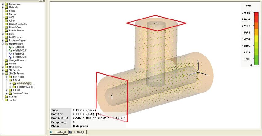
®
CST MICROWAVE STUDIO 2008 – Workflow and Solver Overview

Contents                                                                                                     September 10 , 2007
                                                                                                                                  th

CHAPTER 1 — INTRODUCTION ............................................................................................................... 3
Welcome......................................................................................................................................3
  How to Get Started Quickly .................................................................................................... 3
                                                      ®
  What is CST MICROWAVE STUDIO ?.................................................................................. 3
                                                           ®
  Who Uses CST MICROWAVE STUDIO ? ............................................................................. 5
                                     ®
CST MICROWAVE STUDIO Key Features ...............................................................................5
  General................................................................................................................................... 5
  Structure Modeling ................................................................................................................. 5
  Transient Simulator................................................................................................................. 6
  Frequency Domain Simulator ................................................................................................. 7
  Integral Equation Simulator .................................................................................................... 8
  Eigenmode Simulator ............................................................................................................. 8
  Schematic View ...................................................................................................................... 9
  Visualization and Secondary Result Calculation..................................................................... 9
  Result Export .......................................................................................................................... 9
  Automation ........................................................................................................................... 10
About This Manual.....................................................................................................................10
  Document Conventions ........................................................................................................ 10
  Your Feedback ..................................................................................................................... 10

CHAPTER 2 – SIMULATION WORKFLOW ..............................................................................................11
   The Structure........................................................................................................................ 11
                                                 ®
   Start CST MICROWAVE STUDIO ...................................................................................... 12
   Open the Quick Start Guide.................................................................................................. 13
   Define the Units .................................................................................................................... 14
   Define the Background Material ........................................................................................... 14
   Model the Structure .............................................................................................................. 14
   Define the Frequency Range................................................................................................ 21
   Define Ports.......................................................................................................................... 22
   Define Boundary and Symmetry Conditions ......................................................................... 24
   Visualize the Mesh ............................................................................................................... 26
   Start the Simulation .............................................................................................................. 27
   Analyze the Port Modes........................................................................................................ 30
   Analyze the S-Parameters.................................................................................................... 31
   Adaptive Mesh Refinement................................................................................................... 33
   Analyze the Electromagnetic Field at Various Frequencies.................................................. 36
   Parameterization of the Model.............................................................................................. 41
   Parameter Sweeps and Processing of Parametric Result Data............................................ 47
   Automatic Optimization of the Structure ............................................................................... 54
   Comparison of Time and Frequency Domain Solver Results ............................................... 58
   Summary .............................................................................................................................. 61

CHAPTER 3 — SOLVER OVERVIEW.......................................................................................................62
Which Solver to Use ..................................................................................................................62
General Purpose Frequency Domain Computations .................................................................65
Resonant Frequency Domain Computations .............................................................................69
   Resonant: Fast S-Parameter ................................................................................................ 69
   Resonant: S-Parameter, fields.............................................................................................. 71
Integral Equation Computations ................................................................................................73
Eigenmode (Resonator) Computations .....................................................................................76
Choose the Right Port ...............................................................................................................80
Antenna Computations ..............................................................................................................81
   Simplifying Antenna Farfield Calculations............................................................................. 84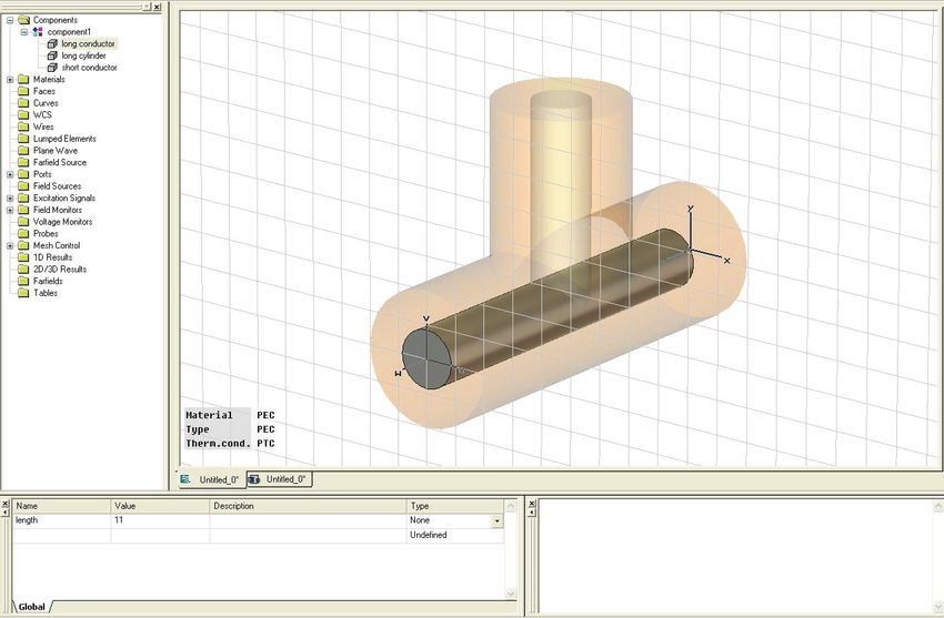
®
2                                   CST MICROWAVE STUDIO 2008 – Workflow and Solver Overview

Digital Calculations ....................................................................................................................85
Add Circuit Elements to External Ports......................................................................................87

CHAPTER 4 — FINDING FURTHER INFORMATION ...............................................................................89
The Quick Start Guide ...............................................................................................................89
Online Documentation ...............................................................................................................90
Tutorials.....................................................................................................................................90
Examples...................................................................................................................................90
Technical Support......................................................................................................................91
History of Changes ....................................................................................................................91

®
CST MICROWAVE STUDIO 2008 – Workflow and Solver Overview                                   3

Chapter 1 — Introduction
Welcome
                                                         ®
     Welcome to CST MICROWAVE STUDIO , the powerful and easy-to-use
     electromagnetic field simulation software. This program combines a user-friendly
     interface with unsurpassed simulation performance.
                                  ®
     CST MICROWAVE STUDIO is part of the CST STUDIO SUITE™. Please refer to the
     CST STUDIO SUITE™ Getting Started manual first. The following explanations assume
     that you already installed the software and familiarized yourself with the basic concepts
     of the user interface.

How to Get Started Quickly

     We recommend that you proceed as follows:

         1.   Read the CST STUDIO SUITE™ Getting Started manual.
         2.   Work through this document carefully. It provides all the basic information
              necessary to understand the advanced documentation.
         3.   Work through the online help system’s tutorials by choosing the example which
              best suits your needs.
         4.   Look at the examples folder in the installation directory. The different
              application types will give you a good impression of what has already been
              done with the software. Please note that these examples are designed to give
              you a basic insight into a particular application domain. Real-world applications
              are typically much more complex and harder to understand if you are not
              familiar with the basic concepts.
         5.   Start with your own first example. Choose a reasonably simple example, which
              will allow you to become familiar with the software quickly.
         6.   After you have worked through your first example, contact technical support for
              hints on possible improvements to achieve even more efficient usage of CST
                                     ®
              MICROWAVE STUDIO .

What is CST MICROWAVE STUDIO®?
                                  ®
     CST MICROWAVE STUDIO is a fully featured software package for electromagnetic
     analysis and design in the high frequency range. It simplifies the process of inputting the
     structure by providing a powerful solid modeling front end which is based on the ACIS
     modeling kernel. Strong graphic feedback simplifies the definition of your device even
     further. After the component has been modeled, a fully automatic meshing procedure is
     applied before a simulation engine is started.
                                                     ®
     A key feature of CST MICROWAVE STUDIO is the Method on Demand™ approach
     which allows using the simulator or mesh type that is best suited to a particular problem.

     All simulators support hexahedral grids in combination with the Perfect Boundary
     Approximation (PBA® method). Some solvers also feature the Thin Sheet Technique
     (TST™) extension. Applying these highly advanced techniques normally increases the
®
4                    CST MICROWAVE STUDIO 2008 – Workflow and Solver Overview

    accuracy of the simulation substantially in comparison to conventional simulators. Since
    no method works equally well in all application domains, the software contains four
    different simulation techniques (transient solver, frequency domain solver, integral
    equation solver, eigenmode solver) to best fit their particular applications. The frequency
    domain solver also contains specialized methods for analyzing highly resonant
    structures such as filters. Furthermore, the frequency domain solver supports both
    hexahedral and tetrahedral mesh types.

    The most flexible tool is the transient solver, which can obtain the entire broadband
    frequency behavior of the simulated device from only one calculation run (in contrast to
    the frequency step approach of many other simulators). This solver is remarkably
    efficient for most kinds of high frequency applications such as connectors, transmission
    lines, filters, antennae and more.

    The transient solver is less efficient for electrically small structures that are much smaller
    than the shortest wavelength. In these cases it is advantageous to solve the problem by
    using the frequency domain solver. The frequency domain solver may also be the
    method of choice for narrow band problems such as filters or when the usage of
    tetrahedral grids is advantageous. Besides the general purpose solver (supporting
    hexahedral and tetrahedral grids), the frequency domain solver also contains fast
    alternatives for the calculation of S-parameters for strongly resonating structures. Please
    note that the latter solvers are currently available for hexahedral grids only.

    For electrically very large structures, volumetric discretization methods generally suffer
                                                                                             ®
    from dispersion effects which require very fine meshes. CST MICROWAVE STUDIO
    therefore contains an integral equation based solver which is particularly suited to
    solving this kind of problems. The integral equation solver uses a triangular surface
    mesh which becomes very efficient for electrically large structures. The MLFMM solver
    technology ensures an excellent scaling of solver time and memory requirements with
    increasing frequencies.

    Efficient filter design often requires the direct calculation of the operating modes in the
    filter rather than an S-parameter simulation. For these applications, CST MICROWAVE
               ®
    STUDIO also features an eigenmode solver which efficiently calculates a finite
    number of modes in closed electromagnetic devices.

    If you are unsure which solver best suits your needs, contact your local sales office for
    further assistance.

    Each solver's simulation results can be visualized with a variety of different options.
    Again, a strongly interactive interface will help you achieve the desired insight into your
    device quickly.

    The last – but not least – outstanding feature is the full parameterization of the structure
    modeler, which enables the use of variables in the definition of your component. In
    combination with the built-in optimizer and parameter sweep tools, CST MICROWAVE
             ®
    STUDIO is capable of both the analysis and design of electromagnetic devices.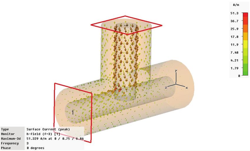
®
CST MICROWAVE STUDIO 2008 – Workflow and Solver Overview 5
Who Uses CST MICROWAVE STUDIO®?
Anyone who has to deal with electromagnetic problems in the high frequency range
®
should use CST MICROWAVE STUDIO . The program is especially suited to the fast,
efficient analysis and design of components like antennae (including arrays), filters,
transmission lines, couplers, connectors (single and multiple pin), printed circuit boards,
resonators and many more. Since the underlying method is a general 3D approach, CST
®
MICROWAVE STUDIO can solve virtually any high frequency field problem.
CST MICROWAVE STUDIO® Key Features
®
The following list gives you an overview of CST MICROWAVE STUDIO ’s main
features. Note that not all of these features may be available to you because of license
restrictions. Contact a sales office for more information.
General
Native graphical user interface based on Windows XP and Vista
Fast and memory efficient Finite Integration Technique
Extremely good performance due to Perfect Boundary Approximation (PBA®) for
solvers using hexahedral grids. The transient and eigenmode solvers also support
the Thin Sheet Technique (TST™). Hexahedral grids are supported by all solvers.
The structure can be viewed either as a 3D model or as a schematic. The latter
allows for easy coupling of EM simulation with circuit simulation.
Structure Modeling
1
Advanced ACIS -based, parametric solid modeling front end with excellent
structure visualization
Feature-based hybrid modeler allows quick structural changes
® ®
Import of 3D CAD data by SAT (e.g. AutoCAD ), Autodesk Inventor , IGES, VDA-
® ® ® ® ®
FS, STEP, ProE , CATIA 4 , CATIA 5 , CoventorWare , Mecadtron , Nastran or
STL files
Import of 2D CAD data by DXF, GDSII and Gerber RS274X, RS274D files
Import of EDA data from design flows including Cadence Allegro® / APD®, Mentor
Graphics Expedition® and ODB++® (e.g. Mentor Graphics Boardstation®, Zuken
CR-5000®, CADSTAR®, Visula®)
Import of 2D and 3D sub models
®
Import of Agilent ADS layouts
®
Import of Sonnet em models (8.5x)
Import of a visible human model dataset or other voxel datasets
Export of CAD data by SAT, IGES, STEP, STL, DXF, DRC or POV files
Parameterization for imported CAD files
Material database
Structure templates for simplified problem description
1
Portions of this software are owned by Spatial Corp. © 1986 – 2007. All Rights Reserved.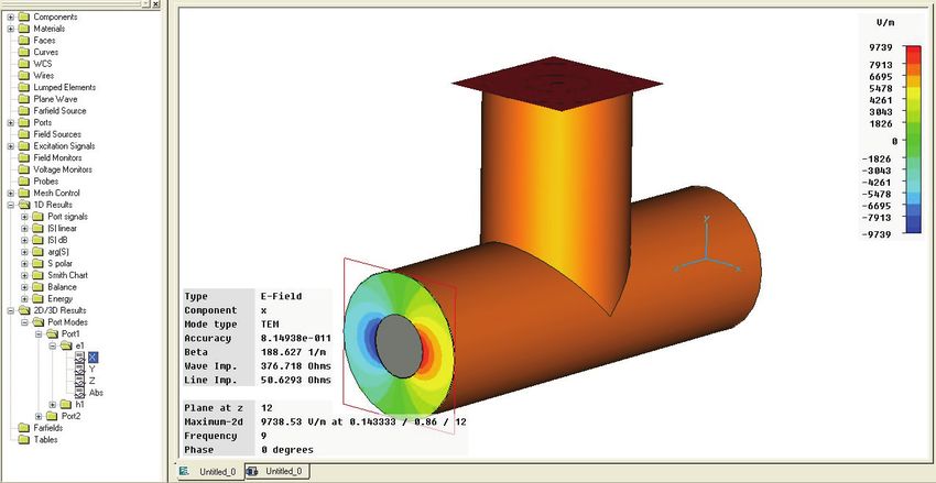
®
6 CST MICROWAVE STUDIO 2008 – Workflow and Solver Overview
Transient Simulator
Efficient calculation for loss-free and lossy structures
Broadband calculation of S-parameters from one single calculation run by applying
DFTs to time signals
Calculation of field distributions as a function of time or at multiple selected
frequencies from one simulation run
Adaptive mesh refinement in 3D
Parallelization of the transient solver run
Support of Acceleware's Accelerator™ A30 and ClusterInABox™ Dual D30 cards
Isotropic and anisotropic material properties
Frequency dependent material properties
Gyrotropic materials (magnetized ferrites)
Surface impedance model for good conductors
Port mode calculation by a 2D eigenmode solver in the frequency domain
Automatic waveguide port mesh adaptation
Multipin ports for TEM mode ports with multiple conductors
Multiport and multimode excitation (subsequently or simultaneously)
Plane wave excitation (linear, circular or elliptical polarization)
®
Excitation by a current distribution imported from SimLab
®
Excitation of external fields imported from Sigrity
S-parameter symmetry option to decrease solve time for many structures
Auto-regressive filtering for efficient treatment of strongly resonating structures
Re-normalization of S-parameters for specified port impedances
Phase de-embedding of S-parameters
Full de-embedding feature for highly accurate S-parameter results
Single-ended S-parameter calculation
High performance radiating/absorbing boundary conditions
Conducting wall boundary conditions
Periodic boundary conditions without phase shift
Calculation of various electromagnetic quantities such as electric fields, magnetic
fields, surface currents, power flows, current densities, power loss densities,
electric energy densities, magnetic energy densities, voltages in time and
frequency domain
Antenna farfield calculation (including gain, beam direction, side lobe suppression,
etc.) with and without farfield approximation at multiple selected frequencies
Broadband farfield monitors and farfield probes to determine broadband farfield
information over a wide angular range or at certain angles respectively
Antenna array farfield calculation
RCS calculation
Calculation of SAR distributions
Discrete edge or face elements (lumped resistors) as ports
Ideal voltage and current sources for EMC problems
Lumped R, L, C, (nonlinear) diode elements at any location in the structure
Rectangular shaped excitation function for TDR analysis
User defined excitation signals and signal database
Simultaneous port excitation with different excitation signals for each port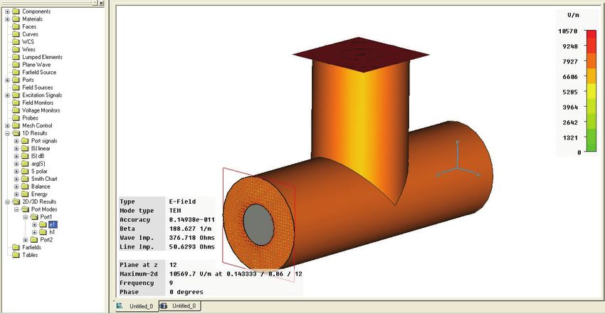
®
CST MICROWAVE STUDIO 2008 – Workflow and Solver Overview 7
Automatic parameter studies using built-in parameter sweep tool
Automatic structure optimization for arbitrary goals using built-in optimizer
Network distributed computing for optimizations, parameter sweeps and multiple
port/mode excitations
Coupled simulations with Thermal Solver from CST EM STUDIO™
Frequency Domain Simulator
Efficient calculation for loss-free and lossy structures including lossy waveguide
ports
General purpose solver supports both hexahedral and tetrahedral meshes
Isotropic and anisotropic material properties
Arbitrary frequency dependent material properties
Surface impedance model for good conductors, Ohmic sheets and corrugated
walls (tetrahedral mesh only)
Inhomogeneously biased Ferrites with a static biasing field (tetrahedral mesh only)
Automatic fast broadband adaptive frequency sweep
User defined frequency sweeps
Continuation of the solver run with additional frequency samples
Adaptive mesh refinement in 3D
Direct and iterative matrix solvers with convergence acceleration techniques
Port mode calculation by a 2D eigenmode solver in the frequency domain
Automatic wave guide port mesh adaptation (tetrahedral mesh only)
Multipin ports for TEM mode ports with multiple conductors
Plane wave excitation with linear, circular or elliptical polarization (tetrahedral
mesh only)
Discrete elements (lumped resistors) as ports
Lumped R, L, C elements at any location in the structure
Re-normalization of S-parameters for specified port impedances
Phase de-embedding of S-parameters
High performance radiating/absorbing boundary conditions
Conducting wall boundary conditions (tetrahedral mesh only)
Periodic boundary conditions including phase shift or scan angle
Unit cell feature simplifies the simulation of periodic antenna arrays or frequency
selective surfaces (tetrahedral mesh only)
Convenient generation of the unit cell calculation domain from arbitrary structures
(tetrahedral mesh only)
Floquet mode ports (periodic waveguide ports)
Calculation of various electromagnetic quantities such as electric fields, magnetic
fields, surface currents, power flows, current densities, power loss densities,
electric energy densities, magnetic energy densities
Antenna farfield calculation (including gain, beam direction, side lobe suppression,
etc.) with and without farfield approximation
Antenna array farfield calculation
RCS calculation (tetrahedral mesh only)
Calculation of SAR distributions (hexahedral mesh only)
Automatic parameter studies using built-in parameter sweep tool
Automatic structure optimization for arbitrary goals using built-in optimizer
Network distributed computing for optimizations and parameter sweeps
Network distributed computing for frequency samples and remote calculation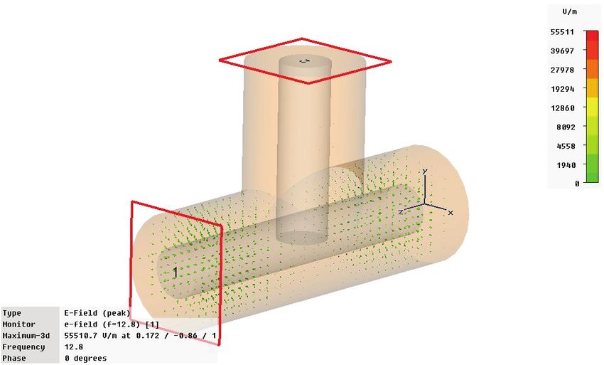
®
8 CST MICROWAVE STUDIO 2008 – Workflow and Solver Overview
Besides the general purpose solver, the frequency domain solver also contains
two solvers specialized on strongly resonant structures (hexahedral meshes only).
The first of these solvers calculates S-parameters only whereas the second also
calculates fields with some additional calculation time, of course.
Integral Equation Simulator
Efficient calculation for loss-free and lossy structures including lossy waveguide
ports
Surface mesh discretization
Isotropic and anisotropic material properties
Arbitrary frequency dependent material properties
Automatic fast broadband adaptive frequency sweep
User defined frequency sweeps
Direct and iterative matrix solvers with convergence acceleration techniques
Higher order representation of the fields including mixed order
Single and double precision floating-point representation
Port mode calculation by a 2D eigenmode solver in the frequency domain
Re-normalization of S-parameters for specified port impedances
Phase de-embedding of S-parameters
Calculation of various electromagnetic quantities such as electric fields, magnetic
fields, surface currents
Antenna farfield calculation (including gain, beam direction, side lobe suppression,
etc.)
RCS calculation
Fast monostatic RCS sweep
Discrete face port excitation
Waveguide port excitation
Plane wave excitation
Farfield excitation
Automatic parameter studies using built-in parameter sweep tool
Automatic structure optimization for arbitrary goals using built-in optimizer
Network distributed computing for optimizations and parameter sweeps
Network distributed computing for frequency sweeps
Eigenmode Simulator
Calculation of modal field distributions in closed loss free or lossy structures
Isotropic and anisotropic materials
Parallelization
Adaptive mesh refinement in 3D
Periodic boundary conditions including phase shift
Calculation of losses and internal / external Q-factors for each mode (directly or
using perturbation method)
Discrete L,C can be used for calculation
Frequency target can be set (calculation in the middle of the spectra)
Calculation of all eigenmodes in a given frequency interval®
CST MICROWAVE STUDIO 2008 – Workflow and Solver Overview 9
Automatic parameter studies using built-in parameter sweep tool
Automatic structure optimization for arbitrary goals using built-in optimizer
Network distributed computing for optimizations and parameter sweeps
Schematic View
Allows for the connection of arbitrary networks to EM ports. These networks can
contain any combination of R/L/C circuit elements, ideal phase shifters, perfect
absorbers, variable reflections, directional couplers, 3dB splitters, CST
®
MICROWAVE STUDIO netlist files and ports.
All circuit simulation capabilities licensed for CST DESIGN STUDIO™ can also be
used within this schematic view.
The schematic view and the 3D view are synchronized automatically.
Visualization and Secondary Result Calculation
Displays S-parameters in xy-plots (linear or logarithmic scale)
Displays S-parameters in smith charts and polar charts
Online visualization of intermediate results during simulation
Import and visualization of external xy-data
Copy / paste of xy-datasets
Fast access to parametric data via interactive tuning sliders
Displays port modes (with propagation constant, impedance, etc.)
Various field visualization options in 2D and 3D for electric fields, magnetic fields,
power flows, surface currents, etc.
Animation of field distributions
Display of farfields (fields, gain, directivity, RCS) in xy-plots, polar plots, scattering
maps and radiation plots (3D)
Display and integration of 2D and 3D fields along arbitrary curves
Integration of 3D fields across arbitrary faces
Automatic extraction of SPICE network models for arbitrary topologies ensuring
the passivity of the extracted circuits
Combination of results from different port excitations
Hierarchical result templates for automated extraction and visualization of arbitrary
results from various simulation runs. These data can also be used for the definition
of optimization goals.
Result Export
Export of S-parameter data as TOUCHSTONE files
Export of result data such as fields, curves, etc. as ASCII files
Export screen shots of result field plots
Export of farfield data as excitation for I-Solver®
10 CST MICROWAVE STUDIO 2008 – Workflow and Solver Overview
Automation
Powerful VBA (Visual Basic for Applications) compatible macro language including
editor and macro debugger
OLE automation for seamless integration into the Windows environment (Microsoft
Office®, MATLAB®, AutoCAD®, MathCAD®, Windows Scripting Host, etc.)
About This Manual
This manual is primarily designed to enable a quick start of CST MICROWAVE
®
STUDIO . It is not intended to be a complete reference guide to all the available
features but will give you an overview of key concepts. Understanding these concepts
will allow you to learn how to use the software efficiently with the help of the online
documentation.
The main part of the manual is the Simulation Workflow (Chapter 2) which will guide you
®
through the most important features of CST MICROWAVE STUDIO . We strongly
encourage you to study this chapter carefully.
Document Conventions
Commands accessed through the main window menu are printed as follows: menu
bar itemÖmenu item. This means that you first should click the “menu bar item”
(e.g. “File”) and then select the corresponding “menu item” from the opening menu
(e.g. “Open”).
Buttons which should be clicked within dialog boxes are always written in italics,
e.g. OK.
Key combinations are always joined with a plus (+) sign. Ctrl+S means that you
should hold down the “Ctrl” key while pressing the “S” key.
Your Feedback
We are constantly striving to improve the quality of our software documentation. If you
have any comments on the documentation, please send them to your local support
center. If you don’t know how to contact the support center near you, send an email to
info@cst.com.®
CST MICROWAVE STUDIO 2008 – Workflow and Solver Overview 11
Chapter 2 – Simulation Workflow
The following example shows a fairly simple S-parameter calculation. Studying this
example carefully will help you become familiar with many standard operations that are
®
important when performing a simulation with CST MICROWAVE STUDIO .
Go through the following explanations carefully, even if you are not planning to use the
software for S-parameter computations. Only a small portion of the example is specific
to this particular application type while most of the considerations are general to all
solvers and application domains.
In subsequent sections you will find some remarks concerning the differences of the
typical procedures for other kinds of simulations.
The following explanations describe the “long” way to open a particular dialog box or to
launch a particular command. Whenever available, the corresponding toolbar item will
be displayed next to the command description. Because of the limited space in this
manual, the shortest way to activate a particular command (i.e. by either pressing a
shortcut key or by activating the command from the context menu) is omitted. You
should regularly open the context menu to check available commands for the currently
active mode.
The Structure
In the example, you will model a simple coaxial bend with a tuning stub. You will then
calculate the broadband S-parameter matrix for this structure before looking at the
electromagnetic field inside this structure at various frequencies. The following picture
shows the current structure of interest (it has been sliced open to aid visualization). The
picture is produced using the POV export option.
Before you start modeling the structure, let’s spend a few moments discussing how to
describe this structure efficiently. Due to the outer conductor of the coaxial cable, the
structure is sealed as if it were embedded in a perfect electric conducting block (apart, of®
12 CST MICROWAVE STUDIO 2008 – Workflow and Solver Overview
course, from the ports). For simplification, you can thus model the problem without the
outer conductor and instead embed it in a perfect conducting block.
®
In order to simplify this procedure, CST MICROWAVE STUDIO allows you to define the
properties of the background material. Anything you do not fill with a particular material
will automatically be filled with the background material. For this structure, it is sufficient
to model the dielectric parts and define the background material as a perfect electric
conductor.
Your method of describing the structure should be as follows:
1. Model the dielectric (air) cylinders.
2. Model the inner conductor inside the dielectric part.
Start CST MICROWAVE STUDIO®
After starting CST DESIGN ENVIRONMENT™ and choosing to create a new CST
®
MICROWAVE STUDIO project, you will be asked to select a template for a structure
which is closest to your device of interest.
For this example, select the coaxial connector template and click OK. The software’s
default settings will adjust in order to simplify the simulation set up for the coaxial
connector.®
CST MICROWAVE STUDIO 2008 – Workflow and Solver Overview 13
Open the Quick Start Guide
An interesting feature of the online help system is the Quick Start Guide, an electronic
assistant that will guide you through your simulation. You can open this assistant by
selecting HelpÖQuick Start Guide if it does not show up automatically.
The following dialog box should now be positioned in the upper right corner of the main
view:
If your dialog box looks different, click the Back button to get the dialog above. In this
dialog box you should select the Problem Type “Transient analysis” and click the Next
button. The following window should appear:
The red arrow always indicates the next step necessary for your problem definition. You
may not have to process the steps in this order, but we recommend you follow this guide
at the beginning in order to ensure all necessary steps have been completed.
Look at the dialog box as you follow the various steps in this example. You may close
the assistant at any time. Even if you re-open the window later, it will always indicate the
next required step.
If you are unsure of how to access a certain operation, click on the corresponding line.
The Quick Start Guide will then either run an animation showing the location of the
related menu entry or open the corresponding help page.®
14 CST MICROWAVE STUDIO 2008 – Workflow and Solver Overview
Define the Units
The coaxial connector template has already made some settings for you. The defaults
for this structure type are geometrical lengths in mm and frequencies in GHz. You can
change these settings by entering the desired settings in the units dialog box
(SolveÖUnits), but for this example you should just leave the settings as specified by the
template.
Define the Background Material
As discussed above, the structure will be described within a perfectly conducting world.
The coaxial connector template has set this typical default value for you. In order to
change these settings, you may make changes in the corresponding dialog box
(SolveÖBackground Material). For this example, you don’t need to change anything.
Model the Structure
The first step is to create a cylinder along the z-axis of the coordinate system:
1. Select the cylinder creation tool from the main menu: ObjectsÖBasic
ShapesÖCylinder ( ).
2. Press the Shift+Tab key and enter the center point (0,0) in the xy-plane before
pressing the Return key to store this setting.
3. Press the Tab key again, enter the radius 2 and press the Return key.
4. Press the Tab key, enter the height 12 and press the Return key.
5. Press Esc to create a solid cylinder (skip the definition of the inner radius).
6. In the shape dialog box, enter “long cylinder” in the Name field.
7. You may simply select the predefined material Vacuum (which is very close to air)
from the list in the Material field. Here we are going to create a new material “air” to
show how the layer creation procedure works, so select the New Material entry in
the list of materials.
8. In the material creation dialog box, enter the Material name “air," select Normal
dielectric properties (Type) and check the material properties Epsilon = 1.0 and Mue
= 1.0. Then select a color and close the dialog box by clicking OK.
9. In the cylinder creation dialog box, your settings should now look as follows:®
CST MICROWAVE STUDIO 2008 – Workflow and Solver Overview 15
Finally, click OK to create the cylinder.
The result of these operations should look like the picture below. You can press the
Space bar to zoom in to a full screen view.
The next step is to create a second cylinder perpendicular to the first. The center of the
new cylinder’s base should be aligned with the center of the first one.
Follow these steps to define the second cylinder:
1. Select the wire frame draw mode: ViewÖ View Options ( ) or use the shortcut
Ctrl+W.
2. Activate the “circle center” pick tool: ObjectsÖPickÖPick Circle Center ( ).
3. Double-click on one of the cylinder’s circular edges so that a point is added in the
center of the circle.
4. Perform steps 2 and 3 for the cylinder’s other circular edge.®
16 CST MICROWAVE STUDIO 2008 – Workflow and Solver Overview
Now the construction should look like the following:
Next replace the two selected points by a point in between the two by selecting
ObjectsÖPickÖMean Last Two Points from the menu.
You can now move the origin of the local coordinate system (WCS) to this point by
choosing WCSÖAlign WCS with Selected Point ( ) from the main menu. The screen
should look like this:®
CST MICROWAVE STUDIO 2008 – Workflow and Solver Overview 17
Now align the w axis of the WCS with the proposed axis of the second cylinder.
1. Select WCSÖRotate Local Coordinates ( ) from the main menu.
2. Select the U axis as rotation Axis and enter a rotation Angle of –90 degrees.
3. Click the OK button.
Alternatively you could press Shift+U to rotate the WCS by 90 degrees around its u axis.
Thus pressing Shift+U three times has the same effect as the rotation by using the
dialog box described above.
Now the structure should look like this:
The next step is to create the second cylinder perpendicular to the first one:
1. Select the cylinder creation tool from the main menu: ObjectsÖBasic
ShapesÖCylinder ( ).
2. Press the Shift+Tab key and enter the center point (0,0) in the uv-plane.
3. Press the Tab key again and enter the radius 2.
4. Press the Tab key and enter the height 6.
5. Press Esc to create a solid cylinder.
6. In the shape dialog box, enter “short cylinder” in the Name field.
7. Select the material “air” from the material list and click OK.
Now the program will automatically detect the intersection between these two cylinders.®
18 CST MICROWAVE STUDIO 2008 – Workflow and Solver Overview
In the “Shape intersection” dialog box, choose the option Add both shapes and click OK.
Finally the structure should look like this:
The creation of the dielectric air parts is complete. The following operations will now
create the inner conductor inside the air.®
CST MICROWAVE STUDIO 2008 – Workflow and Solver Overview 19
Since the coordinate system is already aligned with the center of the second cylinder,
you can go ahead and start to create the first part of the conductor:
1. Select the cylinder creation tool from the main menu: ObjectsÖBasic
ShapesÖCylinder ( ).
2. Press the Shift+Tab key and enter the center point (0,0) in the uv-plane.
3. Press the Tab key again and enter the radius 0.86.
4. Press the Tab key and enter the height 6.
5. Press Esc to create a solid cylinder.
6. In the shape dialog box, enter “short conductor” in the Name field.
7. Select the predefined Material PEC (perfect electric conductor) from the list of
available materials and click OK to create the cylinder.
At this point we should briefly discuss the intersections between shapes. In general,
each point in space should be identified with one particular material. However, perfect
electric conductors can be seen as a special kind of material. It is allowable for a perfect
conductor to be present at the same point as a dielectric material. In such cases, the
perfect conductor is always the dominant material. The situation is also clear for two
overlapping perfectly conducting materials, since in this case the overlapping regions will
also be perfect conductors.
On the other hand, two different dielectric shapes must not overlap each other.
Therefore the intersection dialog box will not be shown automatically in case of a perfect
conductor overlapping with a dielectric material or with another perfect conductor.
Background information: Some structures contain extremely complex conducting parts
embedded within dielectric materials. In such cases, the overall complexity of the model
can be significantly reduced by NOT intersecting these two materials. This is the reason
®
CST MICROWAVE STUDIO allows this exception. However, you should always make
use of this feature whenever possible, even in such simple structures as this example.
The following picture shows the structure as it should currently look:®
20 CST MICROWAVE STUDIO 2008 – Workflow and Solver Overview
Now you should add the second conductor. First align the local coordinate system with
the upper z circle of the first dielectric cylinder:
1. Select ObjectsÖPickÖPick Face ( ) from the main menu.
2. Double-click on the first cylinder’s upper z-plane. The selected face should now be
highlighted:
3. Now choose WCSÖAlign WCS With Selected Face ( ) from the main menu.
The w-axis of the local coordinate system is aligned with the first cylinder’s axis, so you
can now create the second part of the conductor:
1. Select the cylinder creation tool from the main menu: ObjectsÖBasic
ShapesÖCylinder ( ).
2. Press the Shift+Tab key and enter the center point (0,0) in the uv-plane.
3. Press the Tab key again and enter the radius 0.86.
4. Press the Tab key and enter the height –11.
5. Press Esc to create a solid cylinder.
6. In the cylinder creation dialog box enter “long conductor” in the Name field.
7. Select the Material “PEC” from the list and click OK.
The newly created cylinder intersects with the dielectric part as well as with the
previously created PEC cylinder. Even if there are two intersections (dielectric / PEC and
PEC / PEC), the Shape intersection dialog box will not be shown here since both types
of overlaps are well defined. In both cases the common volume will be of type PEC.
Congratulations! You have just created your first structure within CST MICROWAVE
®
STUDIO . The view should now look like this:®
CST MICROWAVE STUDIO 2008 – Workflow and Solver Overview 21
The following gallery shows some views of the structure available using different
visualization options:
Shaded view Shaded view Shaded view
(deactivated working (long conductor (cutplane activated
plane, Ctrl+W) selected) ViewÖCutting Plane,
Appearance of part above
cutplane = transparent)
Define the Frequency Range
The next important setting for the simulation is the frequency range of interest. You can
specify the frequency by choosing SolveÖFrequency ( ) from the main menu:®
22 CST MICROWAVE STUDIO 2008 – Workflow and Solver Overview
In this example you should specify a frequency range between 0 and 18 GHz. Since you
have already set the frequency unit to GHz, you need to define only the absolute
numbers 0 and 18 (the status bar always displays the current unit settings).
Define Ports
The following calculation of S-parameters requires the definition of ports through which
energy enters and leaves the structure. You can do this by simply selecting the
corresponding faces before entering the ports dialog box.
For the definition of the first port, perform the following steps:
1. Select ObjectsÖPickÖPick Face ( ) from the main menu.
2. Double-click on the upper z-plane of the dielectric part. The selected face will be
highlighted:
3. Open the ports dialog box by selecting SolveÖWaveguide Ports ( ) from the main
menu:®
CST MICROWAVE STUDIO 2008 – Workflow and Solver Overview 23
Everything is already set up correctly for the coaxial cable, so you can simply click
OK in this dialog box.
Once the first port has been defined, the structure should look like this:
You can now define the second port in exactly the same way. The picture below shows
the structure after the definition of both ports:
The correct definition of ports is very important for obtaining accurate S-parameters.
Please refer to the Choose the Right Port section later in this manual to obtain more
information about the correct placement of ports for various types of structures.®
24 CST MICROWAVE STUDIO 2008 – Workflow and Solver Overview
Define Boundary and Symmetry Conditions
The simulation of this structure will only be performed within the bounding box of the
structure. You may, however, specify certain boundary conditions for each plane
(Xmin/Xmax/Ymin/Ymax/Zmin/Zmax) of the bounding box.
The boundary conditions are specified in a dialog box you can open by choosing
SolveÖBoundary Conditions from the main menu.
While the boundary dialog box is open, the boundary conditions will be visualized in the
structure view as in the picture above. Added picture above
In this simple case, the structure is completely embedded in perfect conducting material,
so all the boundary planes may be specified as “electric” planes (which is the default).
In addition to these boundary planes, you can also specify “symmetry planes." The
specification of each symmetry plane will reduce the simulation time by a factor of two.
In our example, the structure is symmetric to a yz-plane perpendicular to the x-axis in
the center of the structure. The excitation of the fields will be performed by the
fundamental mode of the coaxial cable for which the magnetic field is shown below:
Plane of structure’s symmetry (yz-plane)
The magnetic field has no component tangential to the plane of the structure’s symmetry
(the entire field is oriented perpendicular to this plane). If you specify this plane as a
®
“magnetic” symmetry plane, you can direct CST MICROWAVE STUDIO to limit the®
CST MICROWAVE STUDIO 2008 – Workflow and Solver Overview 25
simulation to one half of the actual structure while taking the symmetry conditions into
account.
In order to specify the symmetry condition, you first need to click on the Symmetry
Planes tab in the boundary conditions dialog box.
For the yz-plane symmetry, you can choose magnetic in one of two ways. Either select
the appropriate option in the dialog box, or double-click on the corresponding symmetry
plane visualization in the view and selecting the proper choice from the context menu.
Once you have done so, your screen will appear as follows:
Finally click OK in the dialog box to store the settings. The boundary visualization will
then disappear.®
26 CST MICROWAVE STUDIO 2008 – Workflow and Solver Overview
Visualize the Mesh
In a first simulation we will run the transient simulator based on hexahedral grids. Since
this is the default mesh type, we don’t need to change anything here. In a later step we
show how to apply a tetrahedral mesh to this structure, run the frequency domain solver
and compare the results. However, let’s focus on the hexahedral mesh generation
options first.
The hexahedral mesh generation for the structure analysis will be performed
automatically based on an expert system. However, in some situations it may be helpful
to inspect the mesh to improve the simulation speed by changing the parameters for the
mesh generation.
The mesh can be visualized by entering the mesh mode (MeshÖMesh View ( )). For
this structure, the mesh information will be displayed as follows:
One 2D mesh plane is always kept in view. Because of the symmetry setting, the mesh
plane extends across only one half of the structure. You can modify the orientation of
the mesh plane by choosing MeshÖX/Y/Z Plane Normal ( / / ). Move the plane
along its normal direction using MeshÖIncrement/Decrement Index ( / ) or using the
Up / Down cursor keys.
The red points in the model are critical points (so-called fixpoints) where the expert
system finds it necessary to have mesh lines at these locations.
In most cases the automatic mesh generation will produce a reasonable initial mesh, but
we recommend that you later spend some time on the mesh generation procedures in
the online documentation when you feel familiar with the standard simulation procedure.
You should now leave the mesh inspection mode by again toggling: MeshÖMesh View
( ).®
CST MICROWAVE STUDIO 2008 – Workflow and Solver Overview 27
Start the Simulation
After defining all necessary parameters, you are ready to start your first simulation.
Start the simulation from the transient solver control dialog box: SolveÖTransient Solver
( ).
In this dialog box, you can specify which column of the S-matrix should be calculated.
Therefore select the Source type port for which the couplings to all other ports will then
be calculated during a single simulation run. In our example, by setting the Source type
to Port 1, the S-parameters S11, S21 will be calculated. Setting the Source Type to Port
2 will calculate S22 and S12.
In some cases where the full S-matrix is needed, you may also set the Source Type to
All Ports which implies that one calculation run will be performed for each port. However
for loss free, two port structures (like the structure investigated here), the second
calculation run will not be performed since all S-parameters can be calculated from one
run using analytic properties of the S-matrix.
In this case you should compute the full S-matrix and leave All Ports as your Source
type setting.
The S-parameters which are calculated will always be normalized to the port impedance
(which will be calculated automatically) by default. In this case the port impedance will
be approximately
2
138 ⋅ log( ) = 50.58 Ohms
0.86®
28 CST MICROWAVE STUDIO 2008 – Workflow and Solver Overview
for the coaxial lines with the specified dimensions and dielectric constants. However,
sometimes you need the S-parameters for a fixed normalization impedance (e.g. 50
Ohms), so check the Normalize to fixed impedance button and specify the desired
normalization impedance in the entry field below. In this example we assume that you
want to calculate the S-parameters for a reference impedance of 50 Ohms. Note that the
re-normalization of the S-parameters is possible only when all S-parameters are
calculated (Source Type = All Ports).
While solution accuracy mainly depends on the discretization of the structure and can be
improved by refining the mesh, the truncation error introduces a second error source in
transient simulations.
In order to obtain the S-parameters, the transformation of the time signals into the
frequency domain requires the signals to have sufficiently decayed to zero. Otherwise a
truncation error will occur, causing ripples on the S-parameter curves.
®
CST MICROWAVE STUDIO features an automatic solver control that stops the
transient analysis when the energy inside the device, and thus the time signals at the
ports, has sufficiently decayed to zero. The ratio between the maximum energy inside
the structure at any time and the limit at which the simulation will be stopped is specified
in the Accuracy field (in dB).
In this example we will limit the maximum truncation error down to 1% for which you
should keep the default solver Accuracy at –40 dB.
The solver will excite the structure with a Gaussian pulse in the time domain. However,
all frequency domain and field data obtained during the simulation will be normalized to
a frequency independent input power of 1 W.
After setting all these parameters, the dialog box should look like this:
In order to also achieve accurate results for the line impedance values of static port
modes, an adaptive mesh refinement in the port regions is performed as a pre-®
CST MICROWAVE STUDIO 2008 – Workflow and Solver Overview 29
processing step before the transient simulation itself is started. This procedure refines
the port mesh until a defined accuracy value or a maximum number of passes have
been reached. These settings can be adjusted in the following dialog box
SolveÖTransient SolverÖSpecialsÖWaveguide:
Since we want to simulate a coaxial structure with static port modes we keep the
adaptation enabled with its default settings.
You can close the dialog box without any changes and now start the simulation
procedure by clicking the Start solver button. A progress bar will appear in the status bar
which will update you on the solver’s progress. Information text regarding the operation
will appear next to the progress bar. The most important stages are listed below:
1. Analyzing port domains: During this first step, the port regions are analyzed for
the following port mesh adaptation.
2. Port mode calculation: Here, the port modes are calculated during the port mesh
adaptation. This step is performed several times for each port until a defined
accuracy value or a maximum number of passes have been reached.
3. Calculating matrices, preparing and checking model: During this step, the input
model is checked for errors such as invalid overlapping materials.
4. Calculating matrices, normal matrix and dual matrix: During these steps, the
system of equations, which will subsequently be solved, are set up.
5. Transient analysis, calculating the port modes: In this step, the solver calculates
the port mode field distributions and propagation characteristics as well as the port
impedances. This information will be used later in the time domain analysis of the
structure.
6. Transient analysis, processing excitation: During this stage, an input signal is
fed into the stimulation port. The solver then calculates the resulting field distribution
inside the structure as well as the mode amplitudes at all other ports. From this
information, the frequency dependent S-parameters are calculated in a second step
using a Fourier Transformation.
7. Transient analysis, transient field analysis: After the excitation pulse has
vanished, there is still electromagnetic field energy inside the structure. The solver
then continues to calculate the field distribution and the S-parameters until the
energy inside the structure has decayed below a certain limit (specified by the
Accuracy setting in the solver dialog box).®
30 CST MICROWAVE STUDIO 2008 – Workflow and Solver Overview
Step 3 and 4 describe the structure checking and matrix calculation of the PBA mesh
type. In case that the FPBA mesh type is chosen either automatically or manually, these
two steps are represented as follows:
3. Calculating matrices, preprocessing and meshing subdomains: During this
step, your input model is checked and processed.
4. Calculating matrices, computing coefficients: During these steps, the system of
equations, which will subsequently be solved, are set up.
For this simple structure, the entire analysis takes only a few seconds to complete.
Analyze the Port Modes
After the solver has completed the port mode calculation, you can view the results (even
if the transient analysis is still running).
In order to visualize a particular port mode, you must choose the solution from the
navigation tree. You can find the mode in port 1 from NT (stands for the navigation
tree)Ö2D/3D ResultsÖPort ModesÖPort1. If you open this subfolder, you may select
the electric or the magnetic mode field. Selecting the folder for the electric field of the
first mode e1 will display the port mode and its relevant parameters in the main view:
Besides information on the type of mode (in this case TEM), you will also find the
propagation constant (beta) at the central frequency. Additionally the port impedance is
calculated automatically (line impedance).
You will find that the calculated result for the port impedance of 50.63 Ohms agrees well
with the analytical solution of 50.58 Ohms due to the port mesh adaptation. The small
difference is caused by the discretization of the structure. Increasing the mesh density
will further improve the agreement between simulation and theoretical value. However,
the automatic mesh generation always tries to choose a mesh that provides a good
trade off between accuracy and simulation speed.
You can adjust the number and size of arrows in the dialog box, which can be opened
by choosing ResultsÖPlot Properties (or Plot Properties in the context menu).You can also read