Creating Customized CGRAs for Scientific Applications - MDPI
←
→
Page content transcription
If your browser does not render page correctly, please read the page content below
electronics
Article
Creating Customized CGRAs for Scientific Applications
George Charitopoulos 1, *, Ioannis Papaefstathiou 1 and Dionisios N. Pnevmatikatos 2

                                           1   School of Electrical and Computer Engineering, Technical University of Crete, 73100 Chania, Greece;
                                               ygp@ece.auth.gr
                                           2   School of Electric and Computer Engineering, National Technical University of Athens, 15780 Zografou,
                                               Greece; pnevmati@cslab.ece.ntua.gr
                                           *   Correspondence: gcharitopoulos@isc.tuc.gr

                                           Abstract: Executing complex scientific applications on Coarse Grain Reconfigurable Arrays (CGRAs)
                                           offers improvements in the execution time and/or energy consumption when compared to optimized
                                           software implementations or even fully customized hardware solutions. In this work, we explore
                                           the potential of application analysis methods in such customized hardware solutions. We offer
                                           analysis metrics from various scientific applications and tailor the results that are to be used by
                                           MC-Def, a novel Mixed-CGRA Definition Framework targeting a Mixed-CGRA architecture that
                                           leverages the advantages of CGRAs and those of FPGAs by utilizing a customized cell-array along,
                                           with a separate LUT array being used for adaptability. Additionally, we present the implementation
                                           results regarding the VHDL-created hardware implementations of our CGRA cell concerning various
                                           scientific applications.

                                           Keywords: CGRA design; reconfigurable computing; application analysis


Citation: Charitopoulos, G.;
                                           1. Introduction
Papaefstathiou, I.; Pnevmatikatos,               Specialized hardware accelerators of scientific applications often improve the per-
D.N. Creating Customized CGRAs             formance and reduce energy consumption [1]. However, designing and implementing
for Scientific Applications. Electronics   accelerators is a difficult process that requires in-depth knowledge of the application,
2021, 10, 445. https://doi.org/10.33       multiple programming languages, and software tools. Throughout the years, several alter-
90/ electronics10040445                    natives have been proposed in order to make this process easier. The dataflow paradigm
                                           is a promising and well-established alternative towards customized hardware solutions.
Academic Editors: Juan M. Corchado,        Several frameworks that create dataflow graphs (Dataflow Graphs (DFGs)) and map them
Stefanos Kollias and Javid Taheri          on specialized hardware have been proposed [2–5].
Received: 31 December 2020
                                                 Still, the direct mapping of complex DFGs on FPGAs is a tedious process. A more
Accepted: 4 February 2021
                                           convenient alternative target platform is Coarse-Grain Architectures (CGAs). CGAs exploit
Published: 11 February 2021
                                           hardware customization to achieve faster and more energy efficient execution. While they
                                           are appropriate and efficient for many applications (especially with loop-based parallelism),
Publisher’s Note: MDPI stays neu-
                                           their main drawback is the use of fixed and pre-defined hardware that limits their flexibility
tral with regard to jurisdictional clai-
ms in published maps and institutio-
                                           and versatility when compared to other solutions. Coarse-Grain Reconfigurable Architec-
nal affiliations.
                                           tures (CGRAs) are a step towards adding flexibility while retaining many of the efficiency
                                           advantages of CGAs. Being reconfigurable, CGRAs can be re-defined to better match
                                           particular applications or domains. Typical CGRAs are template architectures, with some
                                           degrees of customization.
Copyright: © 2021 by the authors. Li-            A key disadvantage of current CGRA approaches stems from the underlying mapping
censee MDPI, Basel, Switzerland.           algorithm that is used to map the compute functions/operations of the original application
This article is an open access article     on computational nodes of the CGRA architecture. Because early reconfigurable architec-
distributed under the terms and con-       tures, e.g., programmable logic arrays (PLA), typically this mapping used 1-to-1 to fashion
ditions of the Creative Commons At-
                                           a single application gate/function onto a single gate of the architecture. CGRA application
tribution (CC BY) license (https://
                                           mapping, although improved, continues to follow this paradigm limiting the capabilities
creativecommons.org/licenses/by/
                                           of CGRAs. This is due to the design premise of CGRA cells that typically include a single
4.0/).

Electronics 2021, 10, 445. https://doi.org/10.3390/electronics10040445                                     https://www.mdpi.com/journal/electronics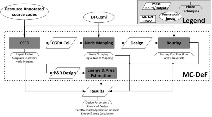
Electronics 2021, 10, 445                                                                                            2 of 23

                            compute element, i.e., an ALU or a micro-processor, an instruction/configuration memory
                            and input/output registers. Additionally despite their massive customization CGRAs still
                            strive to achieve efficient mapping while being as generic as possible. This intentional
                            lack of customized hardware leads to sub-optimal designs in terms of offered acceleration
                            and general execution time. Therefore, we need a CGRA definition framework that is able
                            to: (a) map multiple nodes in one cell and (b) offer customized cell functionality, while
                            maintaining a degree of flexibility.
                                  Before exploring the ways to map applications on CGRAs, one must be able to tailor
                            the underlying framework and be able to construct a feasible and effective way to de-
                            termine how the compute element of the CGRA is defined. In order to achieve this, the
                            researchers focus on application graph analysis used to extract all of the necessary infor-
                            mation. However, this approach may not always be feasible or even effective. The nodes
                            appearing in an application data-flow graph can yield misleading results in terms of fre-
                            quency of appearance when compared to the physical resources used. In this paper, being
                            motivated by this conundrum, we attempt to use preliminary application analysis before
                            building our framework in order to tailor it and create a more accurate algorithm when
                            defining the CGRA cells. This preliminary analysis aids in determining how particular
                            application nodes impact the application’s resource utilization and which nodes appear
                            frequently across applications from different domains. Additionally, because this analysis
                            is integrated in our framework, it aids the user in predicting the resource utilization of an
                            application using only a specific DFG representation, without requiring the expensive and
                            time-consuming step of implementation on the actual platform.
                                  The obtained results are then integrated to our CGRA definition framework, MC-DeF
                            (Mixed-CGRA Definition Framework). MC-DeF is a novel framework that performs all of
                            the necessary steps in order to define a customized CGRA for a target application utilizing
                            a mixed-CGRA architecture. A mixed-CGRA architecture combines the advantages from
                            both the CGRA and the FPGA paradigms, using both a coarse-grain cell structure and
                            an amount of (LUT-based) reconfigurable logic, for added flexibility, connected with a
                            fast and high-bandwidth communication infrastructure. Once defined, the Mixed-CGRA
                            can be implemented either as an ASIC or as an overlay in FPGA technology. The ASIC
                            approach transforms the CGRA into a CGA as the cell functionality cannot be adapted
                            any more. In this case, the array retains some flexibility through the use of the adjacent
                            reconfigurable LUT array. The overlay option creates a reconfigurable CGRA design that is
                            able to map a target application; each new targeted application must be recompiled and
                            configured again on the FPGA. Additionally, by fine-tuning the threshold values that are
                            used by MC-DeF, the user can perform design space exploration in order to find a suitable
                            hardware solution based on area or energy restrictions. Our work stands in the boundary
                            of this space: prototyping with overlays is great for verifying the results of the design-space
                            exploration and an ASIC is the ideal final product. However, the overlay approach still has
                            an advantage from the tools/programming perspective.
                                  This paper expands our previous work [6], making the following contributions:
                            •    an application analysis methodology and results that helped to define the functionality
                                 and fine-tune our framework, and
                            •    a complete description of the created framework and baseline results showcasing its
                                 use, and
                            •    VHDL implementation results of implemented CGRA cells created by MC-DeF.
                                 The rest of the paper is structured, as follows: Section 2 presents related work on
                            the field of CGRA architectures and graph analysis tools, while Section 3 presents the
                            preliminary application analysis and the obtained results. MC-DeF and the targeted Mixed-
                            CGRA are described in Section 4. Section 5 presents a set of evaluations of MC-DeF and
                            CGRA architectures produced with its use. Moreover, in Section 6, we present the VHDL
                            implementation results of MC-DeF created CGRA architectures, and Section 7 concludes
                            our work and presents our final remarks.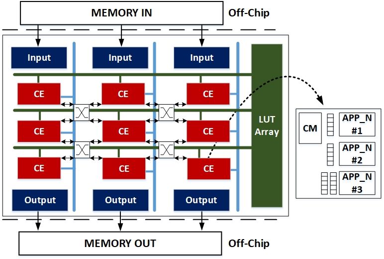
Electronics 2021, 10, 445                                                                                            3 of 23

                            2. Related Work
                                  Several novel Coarse-Grain Architectures have been proposed and the respective field
                            is active for many years. More recently, the emergence of High-Performance Computing
                            and its accompanying applications have led to a rekindling of the CGRA approach. This
                            is due to the large amount of commonalities between HPC applications and also their
                            ability to be easily implemented while using the data-flow paradigm. The presented
                            related work for this paper can be divided in two different parts, works that propose novel
                            CGRA architectures and works that address application analysis and static source code
                            analysis techniques.

                            2.1. CGRA Architectures
                                  Stojilovic et al. present a technique to automatically generate a domain-specific coarse-
                            grained array from a set of representative applications [7]. Their technique creates a shortest
                            common super-sequence found among all of the input applications based on weighted
                            majority merge heuristic. Using this super-sequence, the framework creates a cell array
                            that is able to map the application’s instructions.
                                  In [8], the authors present REDIFINE, a polymorphic ASIC in which specialized
                            hardware units are replaced with basic hardware units. The basic hardware units are
                            able to replicate specialized functionality through runtime re-composition. The high-level
                            compiler invoked creates substructures containing sets of compute elements. An enhance-
                            ment of REDIFINE is presented in [9]. In this work, HyperCell is a framework used to
                            augment the CGRA compute elements with reconfigurable macro data-paths that enable
                            the exploitation of fine grain and pipeline parallelism at the level of basic instructions in
                            static dataflow order.
                                  In [10], the authors present RaPiD, a novel architecture that was designed to implement
                            computation intensive and highly regular systolic streaming applications while using an
                            array of computing cells. The cell consists of a multiplier unit, two ALUs, six registers, and
                            three small memories. The connectivity of RaPiD is based on 10 basses connecting the cells
                            through connectors in a Nearest-Neighbor (NN) fashion.
                                  The SCGRA overlay [11] was proposed to address the FPGA design productivity issue,
                            demonstrating a 10–100× reduction in compilation times. Additionally, application specific
                            SCGRA designs that were implemented on the Xilinx Zynq platform achieved a 9× speed-
                            up compared to the same application running on the embedded Zynq ARM processor.
                            The FU used in the Zynq based SCGRA overlay operates at 250 MHz and it consists of an
                            ALU, multiport data memory (256 × 32 bits), and a customised depth instruction ROM
                            (72-bit wide instructions), which results in the excessive utilization of BRAMs.
                                  QUKU [12] is a rapidly reconfigurable coarse-grained overlay architecture that aims
                            to bridge the gap between soft-core processors and customized circuit. QUKU consists of a
                            dynamically reconfigurable, coarse-grained FU array with an adjacent soft-core processor
                            for system support. QUKU’s evaluation was done using Sobel and Laplace kernels, and the
                            generated QUKU overlay was designed based on datapath merging of the two kernels.
                            QUKU’s datapath merging overlay on top of FPGA fabric paves the way for fast context
                            switching between kernels.
                                  FPCA [13] uses a PE that can either be a Computation Element (CE) or a Local Memory
                            Unit (LMU). FPCA takes advantage of the Dataflow Control Graph of the application to
                            create even more customized elements for the reconfigurable array. Customizable elements
                            are a category of CE’s in the FPCA architecture, with the other being heterogeneous
                            ALUs. The communication network is divided in two different parts, first one is used for
                            transferring data between LMUs and CEs and it is a permutation network, while the other
                            one is a global NN network for general PE communication.
Electronics 2021, 10, 445 4 of 23
2.2. Application Analysis and Static Source Code Analysis
As mentioned, MC-DeF can be used for static source code analysis and for the defini-
tion of application or domain specific CGRAs. Static source code analysis is quite common
in software applications, and many language-specific tools have been released.
LLVM is one of the earliest approaches in source code analysis [14]. LLVM is a
collection of modular and reusable compiler and tool-chain technologies. Through code
analysis, LLVM is able to provide the user transparent support life-long program analysis
and transformation for arbitrary programs. Additionally, LLVM support libraries are able
to perform extensive static optimization, online optimization using information from the
LLVM code, and idle-time optimization while using profile information that is gathered
from programmers in the field.
However, the cases that our work mostly relates to are those of VHDL or hardware
code analysis. A similar approach is that of the SAVE project [15], which is a static source
analysis tool used to measure and compare models to assure the satisfaction of quality
requirements of VHDL descriptions. Similarly to SAVE, RAT [16] uses static source code
analysis in order to maximize the probability of success for an application’s migration
to an FPGA. Efficient post-synthesis resource estimation has been the target of Xilinx
research groups.
Schumacher and Jha formulate a fast and accurate prediction method for the resource
utilization of RTL-based designs targeting FPGAs in [17]. Their work utilizes Verific [18],
which is a parser/elaborator tool, to parse and elaborate RTL-based designs. The presented
results record 60 times faster tool run-time as compared to a typical synthesis process and
slice utilization within 22% of the actual hardware design.
Finally, Quinpu [19] is a novel high-level quantitative prediction modelling scheme
that accurately models the relation between hardware and software metrics, based on
statistical techniques. The error in utilization prediction that is recorded by Quinpu ranges
from 15% to 34%.
3. Application Analysis
A key aspect of this work is to find out whether modern applications can actually
benefit from a coarse-grained reconfigurable architecture. To answer this, the first step of
our research was extensive application analysis. The performed analysis is valuable in
creating the underlying framework that will ultimately be able to map modern scientific
applications in a customized CGRA architecture. Additionally, the intention of the analysis
is to find similarities in the composition of these application or to find “key” functionality
that often appears in the application’s dataflow graph.
This part of the work is done in collaboration with Maxeler Technologies Ltd., a UK-
based HPC company that specializes in Multiscale Dataflow Computing (MDC). Maxeler
offers the Maxeler Platform board solution, which provides the user with multiple dataflow
engines as shared resources on the network, allowing for them to be used by applications
running anywhere in a cluster. In their platform, they also implement various HPC appli-
cations using the MDC paradigm. Their platform allows for high-speed communication
between CPUs and the data-flow engines (DFEs). One Maxeler Dataflow Engine (DFE)
combines 104 arithmetic units with 107 bytes of local fast SRAM (FMEM) and 1011 bytes of
six-channel large DRAM (LMEM) [20].
Maxeler Technologies provided us with a large number of application Dataflow
Graphs (DFG) that we later performed analysis on to find similarities between different
applications or DFG nodes that have a high frequency of appearance. Additionally, we
performed memory analysis, closely monitoring the applications’ needs in memory space
and distinguishing the needed memory in FIFO, RAM, and ROM structures. Finally, we
recorded the input and output nodes of the graphs and measured the amount of input and
output bits at each clock tick in order to determine the I/O needs of the applications at
hand.Electronics 2021, 10, 445 5 of 23
In this section, we first present a preliminary analysis to support our claim that a CGRA
definition framework can indeed provide a viable hardware implementation solution for
modern scientific applications. Subsequently, we will present the four applications used
to demonstrate the usage of Impact Factor, a metric that is used to differentiate a node’s
frequency of appearance in the application’s DFG with the actual resource utilization of said
application. Additionally, we will present the results that were obtained that demonstrate
how the Impact Factor metric can accurately indicate the resource utilization coverage of an
application. The following step in our application analysis is to perform Resource Utilization
Prediction to demonstrate how MC-DeF can accurately predict an application’s resource
utilization by using the application’s data-flow graph and the built-in resource usage node
library created after our Impact Factor analysis. Finally, we steer a discussion summarizing
the key findings and observations of our analysis.
3.1. Preliminary Analysis
We have obtained over 10 commercial applications from Maxeler to perform appli-
cation profiling. MaxCompiler, i.e., the high-level synthesis tool that was developed by
Maxeler, outputs in an .xml file, a detailed graph representation of an application and the
hardware modules it uses, at a higher abstraction level. The modules used in this abstract
representation are high-level constructs, such as adders, counters, multipliers, etc. This
graph representation makes it easier to profile and find similarities among applications
from different domains. In this section, we present the results that were obtained by
resource profiling of these applications.
The preliminary resource analysis has made apparent that the research performed
shows promising results. First, we found that some hardware modules are used in every
profiled application, indicating the necessity of including them in our CGRA cells. The vari-
ance in the numbers is due to the application size, e.g., Spec-FEM 3D is the largest and
most computationally intensive application that we have profiled scoring off the charts
in almost all element categories. As stated, we also opt for fine-grain reconfigurability
within a CGRA cell. This is necessary, because some hardware elements appear in several
applications, but they have a high variance in their number—such as multipliers—as we
can see in Figures 1 and 2. We can see that, generally, FIFO elements are used in all of the
application cases studies; this is clear in Figure 2, where the usage of FIFO elements in all
of the available applications is shown.
Figure 1. Spider graphs reporting the number of adder/subtractor and multiplier elements used in
the 10 sample applications.
The above graphs represent a sub-set of the applications that were used for analysis in
order to define the key features that we wanted to include in MC-DeF. A first observation
that was important in the early stages of development was that the number of instances of
a particular node type does not correlate with high LUT consumption. For example, theElectronics 2021, 10, 445 6 of 23
Hayashi-Yoshida application has 80 nodes that implement some type of logic gate in its
DFG, five adder or subtractor nodes, and two multiplier. However, analysis showed that
logic gate elements only occupy 12% of the total application’s LUT utilization while the
adder and subtractor nodes make up for 94%.
Figure 2. Spider graphs reporting the number of FIFO and logic gate elements used in the 10
sample applications.
3.2. Benchmark Description
We used four scientific applications in order to carry out our preliminary analysis.
The applications used were provided by Maxeler and they were FPGA-ready application
designs. In this section, we will give brief descriptions of the applications used.
• Hayashi-Yoshida coefficient estimator: the Hayashi-Yoshida coefficient estimator [21]
is a measurement of the linear correlation between two asynchronous diffusive pro-
cesses, e.g., stock market transactions. This method is used to calculate the correla-
tion of high-frequency streaming financial assets. Hayashi-Yoshida does not require
any prior synchronization of the transaction-based data; hence, being free from any
overheads that are caused by it. The estimator is shown to have consistency as the
observation frequency tends to infinity. The Maxeler implementation [22] for this
application creates 270 Nodes in total.
• Mutual Information: mutual Information of two random variables is a measure of
the mutual dependence between the two variables. More specifically, it quantifies
the “amount of information” (in units, such as shannons, more commonly called bits)
obtained approximately one random variable, through the other random variable.
This is commonly used in the detection of phase synchronization in time series analysis
in social networks, financial markets, and signal processing. This is the smallest of the
applications analyzed in terms of DFG nodes, with 199 Nodes [23].
• Transfer Entropy: transfer entropy was designed in order to determine the direction
of information transfers between two processes, by detecting asymmetry in their
interactions. Specifically, it is a Shannon information-theory quantity that measures
directed information between two time series. This type of metric is used for mea-
suring, information flow between financial markets or measuring influence in social
networks. Formally, transfer entropy shares some of the desired properties of mutual
information, but it takes the dynamics of information transport into account. Similar
to Mutual Information, the Transfer Entropy has 225 Nodes [23].
• SpecFEM3D: SpecFEM3D [24] is a geodynamic code that simulates three-dimensional
(3D) seismic wave propagation. The algorithm can model seismic waves that pro-
pogate in sedimentary basins or any other regional geological model following earth-
quakes. It can also be used for non-destructive testing or ocean acoustics. This appli-Electronics 2021, 10, 445 7 of 23
cation is the largest and most complex of the ones that we analyzed with MC-DeF.
The DFG of this application contains 4046 Nodes.
• LSH: Locality Sensitive Hashing (LSH) is a common technique in data clustering,
nearest neighbor problem, and high dimension data indexing. The application uses
a hash function h(x) and combination of several hash functions to make sure that
similar data have a larger possibility to be in the same bucket after hashing.
• Capture Client: this is the client’s hardware implementation of a Line Rate Packet
Capture application. The Line Rate Packet Capture is able to perform logging on all of
the incoming data.
• Linear Regression: linear regression is a compute intensive statistical method that
creates a linear model between a scalar response variable y, and one or more explana-
tory variables x. The goal is forecasting or regression for values of y for which no data
are available yet.
• Fuzzy Logic Generator: fuzzy logic extends boolean logic with probability. Instead of
just 1 or 0, every truth value may be any real number between 0 and 1. The numbers
are often replaced by linguistic terms.
• Breast Mammogram: Breast Mammogram is an image segmentation application
used to simplify the representation of an image into something that is easier to
analyze. In this case image segmentation is used to detect microcalcification in the
mammography images in order to detect and treat lesions.
• FFT 1D: a one-dimension Fast Fourier Transformation application. It computes the
discrete Fourier transform, converts signal from its original domain (e.g., time, space)
into the frequency domain. It is widely used in engineering, science, and mathematics.
3.3. Impact Factor and Sub-Graph Analysis Results
As mentioned during our preliminary analysis, we observed that, while certain nodes
appear many times in an application’s DFG, their contribution in the application’s resources
is minimum. This is often the case with logic gates and/or support logic nodes that are
used to transform signals to a different bit-width, dubbed as Reinterpret nodes. By making
this observation we decided to create a metric, called Impact Factor, which will accurately
measure the impact that a DFG node has on the application’s resources.
How repetitive is an application’s DFG is another factor that can aid in the creation
of a CGRA architecture and its definition. The authors, instead of searching for nodes
commonly found in a graph, focus on node sequences that are common, as shown in [7].
In a similar fashion, we made an analysis in order to see whether there are frequently
appearing sub-graphs in our target applications. In this sub-section, we present the results
that demonstrate how, by using the Impact Factor metric, we can observe how resources of
an application are used over a variety of different nodes and memory elements.
First, we create coverage graphs for each of our applications. MC-DeF through
resource analysis computes the Impact Factor of each node in the application DFG. Cumu-
lative impact factors for each resource are collected and presented in graph form for better
readability. These graphs demonstrate how much high-resource utilizing nodes take up
from the total resources used for application implementation. The results of this analysis
are presented in Table 1. With analysis the user can make some first observations regarding
the application, whether it is arithmetically intensive or not, or if different applications
have similarities in their hardware implementation.
In Figure 3, we present the impact factor for each application and FPGA resource
type. We group node resources according to their type, distinguishing arithmetic units
(FP adders, multipliers, etc.), random logic, FIFOs, and memory (BRAMs), and then
plot them in the x axis. The y axis indicates the effect of that node type on each resource
(LUTs, DSPs, BRAMs, Flip-Flops), as expressed in their impact factor. Each coloured bar
shows the percentage of coverage/contribution a node has on a specific physical resource.
For example, in the Hayashi-Yoshida application, the 32-bit FP Adder node utilizes 20% of
the application’s BRAMs (blue bar). The 32-bit FP Multiplier utilizes no BRAM resources;Electronics 2021, 10, 445 8 of 23
as a result, there is no blue bar for that compute element. These results showcase the ability
of MC-DeF to identify the hot-spots in terms of resources in an application. Moreover
information regarding the code line these hot-spots appear is also provided in text form.
In the case of Hayashi-Yoshida, Mutual Information, and Transfer Entropy, we can see
in the corresponding figures that the 32-bit Floating-Point Adders created utilize BRAM
resources. This is evident since the impact factor for the adders is above zero. However,
Synthesis reports that are provided by the vendor tools do not stress this fact, but state that
all of the BRAM utilization is for memory purposes. This information is not provided to
the user in the post-synthesis report. However, in the MC-DeF resource analysis report,
the user can see the correct BRAM utilization and the line/node that it originates from.
Table 1. Synthesis (Dataflow Graph (DFG) nodes) and Overall (FPGA resources) resource utilization
for each application.
Resource Utilization
Applications FIFOs Add. Sub. Mult. Div.
Hayashi-Yoshida 22 1 5 2 0
Mutual Information 15 6 9 15 9
Transfer Entropy 17 6 9 15 9
SpecFEM3D 530 193 18 271
Logic Gates LUT DSP BRAM
Hayashi-Yoshida 48 3912 4 0
Mutual Information 23 17,533 24 2
Transfer Entropy 17 17,677 24 1
SpecFEM3D 227 315,475 1080 1180
Figure 3. Impact Factor for each application and FPGA resource type (LUTs, DSPs, BRAMs, Flip-
Flops) is presented. Each bar depicts the contribution of a specific compute or memory element
among the different physical FPGA resources.Electronics 2021, 10, 445 9 of 23
Regarding sub-graph analysis, we created an algorithm to extract sub-graphs from
the DFG of the application that are frequently based on a frequency threshold. The nodes
that are selected for frequent sub-graphs are identical in terms of functionality as well as
for the operands’ bitwidth. With this process, we try to extrapolate information regarding
the connectivity of the application’s design.
During our research, we concluded that sub-graphs that have a high occurrence
frequency consist of simple logic gates and/or reinterpret nodes. On the other hand, by
broadening the search space in lower frequency of appearance, we were able to discover
more complex constructs and sub-graphs that utilize more resources. Table 2 shows
the results obtained for each application’s highest frequency and highest utilization sub-
graphs.
Table 2. Frequent sub-graph characteristics for each application.
Highest Frequency
Resource Utilization
Applications Frequency #Nodes
(LUT, DSP, BRAM)
Hayashi-Yoshida 11 2 2 0 0
Mutual Information 9 2 2 0 0
Transfer Entropy 11 2 2 0 0
SpecFEM3D 162 3 4 0 0
Highest Utilization
Resource Utilization
Frequency #Nodes
(LUT, DSP, BRAM)
Hayashi-Yoshida 4 7 615 2 0
Mutual Information 4 2 615 2 0
Transfer Entropy 5 2 615 2 0
SpecFEM3D 95 2 290 0 4
The highest frequency sub-graphs for all applications consist of simple nodes, like
reinterpret nodes, logic gates, slices, and multiplexers. The highest utilization sub-graphs
usually contain complex abstract nodes, like FIFOs and subtractors (Mutual Information,
Transfer Entropy, and Hayashi Yoshida), or add-multiply chains (SpecFEM3D). In the case
of Hayashi-Yoshida, besides complex abstract nodes, the highest utilization sub-graph
contains low-resources nodes, like multiplexers and reinterpret nodes.
3.4. Resource Utilization Prediction
The aforementioned analysis yields another attribute of MC-DeF, that of utilization
prediction. During the initial steps of our analysis we used a Maxeler Compiler generated
resource annotated source code file to extrapolate information regarding the DFG nodes’
resource utilization. The resource annotated source code provides information on physical
resources (LUTs, Flip-Flops, BRAMs, DSPs) used per line. However, the user cannot
perform a one-to-one match between the physical resources and nodes. This is due to the
fact that many nodes can be instantiated in one line of code.
However, MC-DeF is able to perform application analysis and cell definition without
the source-annotated code. Through extensive testing, we were able to measure the LUT,
DSP, and BRAM resource utilization of key computation elements, such as adder nodes,
multiplier nodes, etc. Based on this pre-analysis, MC-DeF is able to extrapolate data for
unknown nodes and create a “resource library” of nodes that is also bit-width dependent.
Accordingly, for every new application entered by the user, if no source annotated code
exists, MC-DeF uses its own “resource library” during the CSFD phase.
This “resource library” has lead our research in an interesting side-product, resource
utilization prediction. By only the application’s DFG, the user can have an early predictionElectronics 2021, 10, 445 10 of 23
of how much resources will be utilized. This can be prove to be useful in early stages of
application development and for scheduling algorithms developers. In order to examine
the validity of the prediction performed by MC-DeF, we test its accuracy when compared
to a commercial tool. The current Maxeler framework uses the Altera Synthesis toolchain.
Based on the baseline models, the resource annotated source files, and the MC-DeF’s
“resource library”, we measured MC-DeF’s error margin from 5–10% as compared to the
actual synthesized design, while the execution time of the resource analysis step is 40
times faster than the Synthesis process. When comparing with other resource prediction
tools, we find that MC-DeF achieves 2–3 times better error margin as compared to [17] and
Quinpu [19], while being slower when compared to [17].
Additionally, a case can be made on the amount of abstract nodes covered by the
highest frequency sub-graphs as compared to the total nodes of the application. On average,
according to the applications analyzed, the highest frequency sub-graphs cover ≈ 10% of
the total application nodes.
The resulting frequent sub-graphs can aid the user in identifying patterns in the high-
level code and common sequences of arithmetic operations. However, frequent sub-graphs
are more useful when considering a CGRA implementation of the application. First a high-
utilization sub-graph, when replicated, can cover a large amount of the application’s total
resources. For example, the Hayashi-Yoshida highest utilization sub-graph uses 615 LUTs
and appears four times; this results in an impact factor of 57%. The other applications’
high-utilization subgraphs have an impact factor of approximately 10%. The nodes used
for the common sub-graph combined with the ones that were discovered as high impact
factor nodes during the resource analysis can lead to an almost 100% application coverage
and create a CGRA “cell” that is capable of accommodating the target application.
3.5. Discussion
So far, we have described the preliminary analysis used to tailor MC-DeF and provided
results regarding the Impact Factor metric and the Sub-graph mining process. The applica-
tions that are used for our experiments can be divided into three categories, a large complex
application (SpecFEM3D), two similar applications (Transfer Entropy, Mutual Information),
and a low resources application (Hayashi-Yoshida).
The execution time of MC-Def is dependant on the DFG size and the frequency
threshold that is applied for sub-graph mining. For the small and medium sized graphs
used (Hayashi Yoshida, Mutual Information, and Transfer Entropy), execution time was
recorded at an average of 10 s, while, for SpecFEM3D, was 30 s when the frequency
thresholds for frequent occurring sub-graphs was set at 95. We observed that, when
lowering the frequency threshold, execution time further increased since the tool needed
to process and extrapolate an increasing number of sub-graphs.
When considering the Impact Factor analysis results, we make the following observa-
tions: (a) In small or medium applications it is evident which nodes have a clear impact to
the physical resource utilization, and (b) BRAM modules are primarily used by memory re-
lated nodes, such as FIFOs and RAM/ROM memories, with a small fraction used by some
floating-point arithmetic nodes, and (c) DSP resources are solely used by floating-point
multiply and division units.
Point (a) is evident in the Hayashi-Yoshida coverage graph, where we can see most
of the LUT resources on floating point addition, the impact factor of the 32-bit adder
node is 86%. Transfer Entropy and Mutual Information spend their LUT resources in
a common way. Most of the LUTs are utilized for floating-point division and addition
nodes, a combined impact factor of 78%. Additionally, point (b) can also be observed
in the Hayashi-Yoshida application, 20% of the available BRAMs are used for arithmetic
operations, with the rest being used for pipelining, input/output and FIFOs. Finally,
for point (c), we can see that in the Transfer Entropy coverage graph floating-point division
units use more than 60% of the DSPs, while the rest are used by floating-point multipliers.Electronics 2021, 10, 445 11 of 23
The same observations hold for our largest application, SpecFEM3D. Nodes that
perform 60-bit floating-point addition and multiplication take up to 90% of the applications
total LUTs used, when we include the 64-bit floating-point units, and the impact factor
increases to 96.7%. The multiply units used for 60-bits operation combined with the ones
for 64-bits use is 99.9% of the application’s DSPs. The BRAM usage distribution is unique,
since, in the Maxeler case, BRAM circuitry is used for memory related nodes, i.e., FIFOs
and RAM/ROM memories, but also from some addition units. The impact factor of FIFO
nodes on the BRAMs is 67.56% and, for RAM/ROM memories, is 14.18%, while the rest
spans across the addition units of the DFG.
The analysis that was performed by our tool shows how physical resources are
distributed across the application’s nodes offer unique information not provided by other
vendor tools. Moreover, the prediction error recorded by MC-DeF is, on average, within
10% of the application’s actual resource utilization, the smaller compared to other related
works in the field [17,19]. Finally, after analyzing four scientific application, we have
demonstrated that:
• MC-DeF helps the user identify, abstract nodes with the highest contribution to the
application’s resource utilization,
• MC-DeF finds not only frequent, but also sub-graphs with high resource utilization,
• the high impact factor nodes and sub-graphs discovered by MC-DeF can create a
CGRA capable for accommodating the target application, and
• MC-DeF helps the user identify similarities in applications without looking at their
high-level source files.
4. Mixed-CGRA Definition Framework
This section presents the Mixed-CGRA Definition Framework and its associated
processes and algorithms, this is done in order to offer the reader a holistic view of
the framework.
Figure 4 shows the complete process carried out by MC-DeF. The grey rectangles
denote the phases of MC-DeF: (a) CSFD phase (Section 4.1) decides on the contents of the
CGRA cell, (b) the Node mapping phase (Section 4.2) creates a modified DFG graph using
the resulting CGRA cell, (c) the Routing phase (Section 4.3) creates a mapped and routed
design that is ready to place on an FPGA device and, (d) Energy & Area Estimation phase
(Section 4.4) presents the user with estimates of the created CGRA design.
Figure 4. The MC-DeF flow with its associated phases and techniques.
Figure 5 shows the resulting CGRA design. The figure depicts the cell array (CE
grid), the connectivity network, and the adjacent LUT array that enables mapping arbitraryElectronics 2021, 10, 445 12 of 23
functions that are not very common in the application. The picture also depicts the internal
structure of the cell with the network configuration memory (CM), the implemented
application nodes (APP_N), and the necessary FIFOs.
Figure 5. Structure of the proposed Coarse Grain Reconfigurable Arrays (CGRA).
4.1. Cell Structure and Functionality Definition (CSFD) Phase
The majority of current CGRA architectures use a static and pre-defined set of compute
elements, soft-core processors, and/or ALU elements coupled with instruction memories
to create a compute cell. While these kind of approaches have proven highly flexible
and are general enough to map a wide range of application they lack in: (a) application
scaling (b) resource utilization, and (c) the total number of operation performed in parallel.
With MC-DeF we opt towards a CGRA cell able to perform more than one operation in
parallel, includes high abstraction hardware modules and is able to implement a wide
range of applications through cell-network communication reconfiguration.
MC-DeF utilizes three techniques to create highly customized cells optimized to the
target application’s characteristics. The first one is the Impact Factor metric, introduced
in [6], which denotes the estimated resource impact that a DFG node has on the actual
resource utilization of the application, i.e., percentage of LUTs, FIFOs, BRAMs, and DSPs
used by a node, over the total resource usage of the application. Nodes with high Impact
Factor are labeled for inclusion in the cell structure.
Frequent Sub-Graphs Discovery is the second technique, a process baring strong
similarity to the one that was used to identify frequent chains of instructions [25]. In [6],
the authors run a modified version of GraMi [26], an algorithm for extracting frequent
sub-graphs from a single large graph. A graph is only extracted if it exceeds a frequency
and a resource utilization threshold, thus limiting the search space to sub-graphs that have
high occurrence frequency and use the most hardware resources.
The third technique deals with a critical issue in CGRA design: often times nodes have
the same sequence of operations, but apply it on different bit-widths. The naive approach
considers these nodes as separate, leading to CGRA designs that are harder to route due
to cell heterogeneity. To address this, we include in the CSFD phase Node Merging; an
algorithm that is designed to find whether two nodes with the same functionality should
be merged under the same bit-width and what the optimal bit-width for the current
application is described in detail in [27]. We use two metrics for Node Merging: theElectronics 2021, 10, 445 13 of 23
bit-width difference between the two nodes and the Percentage Gain of merging these
two nodes.
Through the CSFD phase MC-DeF decides which DFG nodes will be implemented
within the CGRA cell and ensures that the functionality of the CGRA-cell is beneficial in
terms of resources, frequency of occurrence in the DFG, and bandwidth achieved among
cell communication. The threshold values applied are subject to change according the user
needs and design restrictions.
4.2. Node Mapping
Node mapping is the process of assigning DFG nodes of an application in CGRA
cells. However, CGRA cells may contain multiple independent or chained functions, which
makes the problem of mapping nodes to cells a difficult algorithmic process.
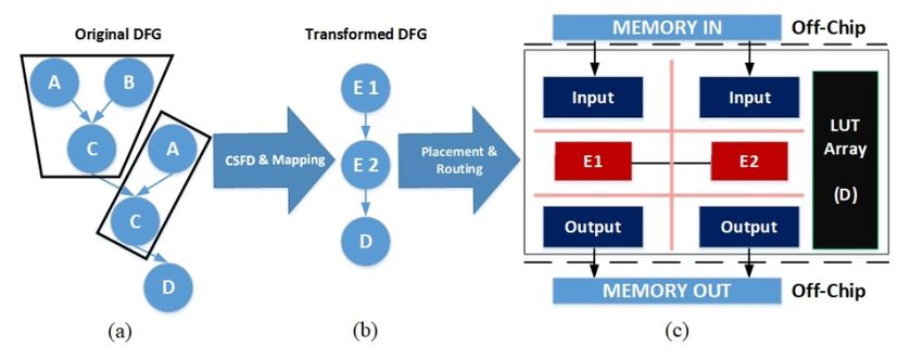
We implement a novel Node Mapping algorithm in order to efficiently allocate the
DFG nodes on the CGRA cells. Starting from an application DFG using nodes N = A, B,
C, D, MC-DeF decides on the contents of the CGRA cell on the CSFD phase, the resulting
CGRA cell contains one stand-alone node and a sub-graph (right arrow notation denotes
a sub-graph inclusion in the CGRA cell), i.e., E = A → C, B. In the mapping phase of
MC-DeF, we want to create a new graph that emits the nodes included in the CGRA cell
and substitutes them with a new node, Node E, which describes the resulting CGRA cell,
as shown in Figure 6. Ultimately, the hardware elements included in E1 and E2 are the
same but their utilization differs, as seen only with the sub-graph A → C being used in
E2. Node Mapping finds and evaluates possible coverings/mappings of the DFG using two
cost functions:
• Unutilized cell resources: this cost function measures the amount of unused resources
among all of the CGRA cells. A CGRA cell consisting of three nodes, with only two of
them used, will have unutilized cell resources count equal to one.
• Connections between cells: this cost function measures wire connections between
different CGRA cells.
Figure 6. Node Mapping in the MC-DeF. (a) The CSFD phase decides on the CGRA cell contents,
(b) Mapping creates a DFG using the new node E, the functionality of which is equivalent to the
CGRA cell defined, (c) Placement and Routing phases place the nodes in a CGRA grid and decide
the connectivity between them.
The mapping algorithm considers all of the nodes or chains of nodes implemented
in the customized CGRA cell. If the CGRA cell contains a sub-graph, i.e., two or more
nodes explicitly connected, the algorithm finds all the corresponding nodes (nodes between
the source and destination nodes and then places them in a cell structure. Subsequently,
for each of the nodes placed already in the cell, the algorithms records all of the DFG nodes
that are adjacent, i.e., with a direct connection, or close, with minimum distance, to the
ones already in the cell, and stores them in the extra_nodes structure. These nodes are then
checked against all other placed nodes in the cell array, and the ones already placed are
removed from the structure. The remaining nodes are all inserted in the cell providedElectronics 2021, 10, 445 14 of 23
adequate available logic, or, if not, the algorithm chooses, at random, which ones to insert
in the current CGRA cell.
At this stage, non-inserted nodes are stored and prioritized for inclusion in subsequent
runs of the mapping algorithm. The same process is repeated if the current processed CGRA
cell logic is not a chain of nodes. For each unique mapping created, the algorithm measures
the Unutilized cell resources and the Connections between cells cost functions and chooses
the mapping that best minimizes them. This process is repeated for 100 mappings. This
number is a design time parameter that can be fixed accordingly by the user, depending on
the required effort tht was spent by the framework to find an optimal solution. Finally, with
the use of the search_non_mapped function, the mapping process records all of the nodes not
able to be placed within a cell, these node will later be placed in the LUT structure available.
Even though some nodes are not directly mapped to CGRA cells, e.g., node D in
Figure 6, CSFD phase strives to ensure that these node are but a small fraction of the total
resources used by the application. However, it is necessary to map these nodes in the
Mixed-CGRA design. MC-DeF offers the user two alternatives for “rogue” nodes.
• LUT array: an adjacent LUT array able to accommodate all the DFG nodes not directly
mapped to the cell logic.
• LUTs-in-cell: the remaining rogue nodes are implemented in small LUT array structures
placed inside the CGRA cells.
The LUT-array approach is straightforward in terms of implementation from MC-DeF.
First, during the Node Mapping phase any node that is not included in the cell array is
labeled for LUT-based implementation on the LUT-array. Subsequently, the Routing phase
establishes the grid network that is responsible for transferring data to and from the LUT-
array. Node implementation and mapping within the LUT array structure is similar to
mainstream FPGAs. The LUT array is not treated as a CE, because the intention is to offer
a degree of reconfigurability that CGRA cells do not.
The LUTs-in-cell (L-i-C) option is more complex. First, we have to take the size of
the individual LUT-structures into consideration and keep an almost uniform distribution
among the CGRA cells. The inspiration for this idea was the Stitch architecture [28] and its
ability to create heterogeneous and configurable core-tiles. Additionally, we ideally want
to place rogue nodes inside cells that have a direct connection with, e.g., RN 1 takes inputs
and gives output to nodes that are placed in Cell 2, so we intuitively want to place it in the
cell’s 2 LUT structure.
For more complex decisions, we invoke the cost functions implemented in the Routing
phase of MC-DeF and make placement decisions accordingly. The routing cost functions
are taken in consideration, because, for rogue nodes, there are no resource-related restrictions.
For routing purposes, a separate network is implemented working transparently from the
cell network. The two networks communicate via dedicated buffers.
The algorithm tries to find a mapping that minimizes the cost functions and terminates
its execution after discovering at least 100 mappings. Each mapping is different, depending
on which of the adjacent nodes will be selected for cell inclusion. The above number is
empirically used through experimentation with the applications used to evaluate MC-DeF.
A further increase of the number of minimum mappings discovered could yield better
overall mapping results but at the cost of increased execution time. This number can be
tailored by the end user of the framework.
4.3. Cell Routing
In this phase, MC-DeF establishes the connections that are needed to route the cell
array, as well as the input/output infrastructure of the design. The Routing phase of MC-
DeF uses two cost functions in order to create designs with low communication overhead:
the number and size of synchronization FIFOs used in each cell and the distance of two
communicating cells.
Dataflow execution dictates that operands arrive at compute nodes synchronized.
However, operands from different paths may observe different compute and communica-Electronics 2021, 10, 445 15 of 23
tion latencies. MC-DeF uses synchronization FIFOs where needed to re-time inputs in each
CGRA cell. Synchronizing cell-node inputs could be remedied—but not fully solved—by
latency-aware mapping of the cells; however, this would lead to increasing the overall
latency of all the cell-array. By inserting synchronization FIFOs inside the cells, we ensure
unobstructed parallel and pipelined execution.
Cells are recognised by their position in the array, i.e., vertical and horizontal coordi-
nates. For two cells that exchange data between them, their distance is equal to the number
of D-Mesh bi-directional crossbar switches between them. For example, the distance of
cell A (0, 0) and cell B (2, 1) is 2. After calculating the cell distance between two connect-
ing cells, the synchronization FIFOs are formulated accordingly. Distance between cells
and Input/Output nodes and the LUT array is three, since communication is achieved
over the slower grid network. The distance between the nodes within the LUT array is
not considered.
These cost functions are used for improving the communication infrastructure. The next
step of the routing process is to minimize them using a Mapping Improvement algorithm.
Through multiple trials, we observed that simultaneously minimizing both of the metrics
is not possible. Instead, we focused the minimization on the metric with the largest vari-
ance among its values. Consequently, the Mapping Improvement Algorithm focuses on
minimizing the distance of two communicating cells.
For the two cells mentioned before, we move one of them along the axis that shows the
largest distance. For example, moving Cell A to the (1, 0) position reduces the distance by
1. After this cell movement, we need to re-calculate the average distance per cell compared
with the previous value and perform more cell movements if necessary. The process is
repeated until a local minimum value is found, after a finite number of movements.
4.4. Area & Energy Estimations
The overall cost of the resulting CGRA architecture is evaluated by measuring the area
of the resulting architecture and the energy consumption. Similar to other state of the art
related works [29,30], we estimate the area occupancy of our architecture while assuming a
7 nm lithography technology. Thus, a 6T SRAM bit cell unit’s size is 30 nm2 , i.e., 38.5 Mb
in 1 mm2 . For example, a 1 k × 8 bit FIFO will occupy approximately 250 µm2 , while
the area needed to implement a fused double precision Multiply-Accumulate on 7 nm is
0.0025 mm2 . Additionally, we consider two 19.5 mm2 Input/Output infrastructures at the
top and bottom of the CGRA with 13 mm length and 1.5 mm width. Additionally, the LUT
array area is calculated based on [31,32]. The numbers reported by the area evaluation
phase of MC-DeF are: CGRA-only, CGRA+I/O and Total (CGRA+I/O+LUT) Area in mm2 .
Calculating the energy consumption of the resulting Mixed-CGRA design is based
on the individual computing elements used. Bill Dally, in [33], shows how the 64-bit
double precision operation energy halved from 22 nm to 10 nm. Additionally, in [34], Dally
et al., accurately measure the energy consumption of several electronic circuits on a 10 nm
lithography technology. The numbers reported in this study are the basis of our energy
consumption estimations and they constitute a pessimistic estimate for a 7 nm lithography.
In Tables 3 and 4, we present the area and energy estimations that were considered
by our MC-DeF framework. The nodes presented in these tables are the ones found in the
application DFGs used for our studies and initial calibration of the MC-DeF. The system
interconnect access requires 1000 pJ. Additionally, in the MC-DeF energy and area con-
sumption estimations, we assume 100% utilization of the Cell and LUT arrays on a fully
utilized pipeline dataflow path. These values are worst case scenarios, so they correspond
to highly overestimated scenarios. Additional optimizations at the implementation level
would allow for more efficient designs.Electronics 2021, 10, 445 16 of 23
Table 3. Energy Consumption of Electronic Circuits used in MC-DeF
Circuit (32-Bit Double Percision) Energy (pJ)
Node Add/Sub 10
Node Multiply 9
Node Division 13
Logic Gates Nodes 0.5
64-bit read from an 8-KB SRAM 2.4
Data movement between cells 0.115 pJ/bit/mm
Table 4. Area Occupancy Estimations of Electronic Circuits used in MC-DeF
Circuit Area (µm2 )
Node Add/Sub
2500
Node Multiply/Divide
FIFO (Bits)
Width Depth
≤8 ≤1000 250
>8 ≤1000 250
≤8 >1000 [ Depth/1000] × 250
>8 >1000 [ Depth/1000] × [Width/8] × 250
4.5. Discussion
The Mixed-CGRA reconfigurable designs that are produced by MC-DeF are tech-
nology agnostic. Two main avenues for the implementation of these designs are (a) on
FPGAs and (b) as custom ASICs. The former option is typical in the CGRA research field
and we can take advantage of the FPGA reprogramming and use MC-DeF results as an
overlay structure. The overlay, together with the data transfer protocol and framework,
forms a complete system. The latter option is to produce a highly optimized, one time
programmable accelerator for a specific application domain. However, the certain level
of reconfigurability remains in the LUT array and the programmability of the Cell Array
switch boxes.
Throughout its execution, MC-DeF uses several metrics, thresholds, and cost-functions.
In Table 5, we list the name, type, and MC-DeF phase each of them is used. The parameters
used can be divided in two categories: those used to create a more compact and resource
efficient array and those that are used to create a fast and high bandwidth communica-
tion framework.
The applied threshold values can be used for design space exploration in order for
the user to find a hardware solution that is tailored to either area or energy restrictions.
This feature is also aided by the fast execution and simulation times of MC-DeF averaging
below two minutes.Electronics 2021, 10, 445 17 of 23
Table 5. MC-DeF metrics, thresholds and cost-functions. Entries annotated with ∗ are used for
Communication infrastructure optimization, and with † for CGRA array optimization.
Name Type MC-DeF Phase
CSFD
Impact Factor † metric
Application Analysis
Utilization of frequently CSFD
threshold
occurring sub-graphs † Sub-graph Discovery
Frequency of frequently CSFD
threshold
occurring sub-graphs † Sub-graph Discovery
metric CSFD
Percentage Gain †
(threshold applied) Node Merging
metric CSFD
Bit-difference †
(threshold applied) Node Merging
Connections between Cells ∗ cost function Mapping
Unutilized Cell Resources † cost function Mapping
Cell Distance ∗ cost function Routing
Number and Size
cost function Routing
of Sync. FIFOs ∗
5. MC-DeF Baseline Results
We verified MC-DeF’s functionality using nine scientific applications’ DFGs that were
provided by Maxeler Ltd. Initially, MC-DeF determines the structure and functionality of a
CGRA cell, as well as the in-cell LUTs or the adjacent LUT-array used for mapping non-cell
nodes. Afterwards, the MC-DeF continues to map the nodes to cells and eventually specify
the connectivity network of the design and finalize the mapping of the cells while using
the novel Mapping Improvement Technique. Finally, MC-DeF provides the user with area
occupancy and energy consumption estimations and presents a final report.
Using the finalised MC-DeF reports from each of the nine applications, we report
the customized CGRA cell functionality, the size of the cell array, the mapping of non-cell
nodes, the utilization of a cell in the array, i.e., average output/cell, and the achieved clock
frequency. Also, MC-DeF provides the user with insight regarding the communication
network’s utilization we report the average distance/cell, synchronization FIFO size/cell
and finally the internal bandwidth recorded. Energy consumption of the resulting designs
is calculated using the amount of input data of each application supplied by the user.
Energy consumption estimations is based on the amount of floating-point operations
performed and the cell array’s network energy consumption, i.e., the energy required for
transferring the data through the cell array. Each cell of the cell array performs pipelined
and parallel operations. MC-DeF design can be implemented either as a overlay or a
standalone design following the architecture shown in Figure 6, for this case the target
board for our designs is a Stratix V FPGA. MC-DeF design results for all nine applications
are presented in Table 6.
For each of the cell structures implemented, we calculate the energy consumption
and area occupancy based on the tables presented in Section 4.4, for nodes that do not
appear in this section we use energy and area estimation as derived from simple VHDL
implementation of the node, such as equality nodes. The right arrow annotation between
certain nodes denotes a sub-graph inclusion in the cell, e.g., NodeEq → NodeAnd in the
Hayashi Yoshida application.
For the majority of applications, the communication infrastructure is configured
using 32-bit channels (breast mammogram and client server use 8 and 24-bit channels
respectively). MC-DeF decides on the communication infrastructure after enumerating
input and output bit-widths for each node implemented in the cell array. Also this choice
is made considering that the majority of operations performed for each application, which,
in most cases, is 32-bit double precision floating-point.You can also read