Global Estimation of Biophysical Variables from Google Earth Engine Platform - MDPI
←
→
Page content transcription
If your browser does not render page correctly, please read the page content below
remote sensing
Article
Global Estimation of Biophysical Variables from
Google Earth Engine Platform
Manuel Campos-Taberner 1, * ID , Álvaro Moreno-Martínez 2,3 ID , Francisco Javier García-Haro 1          ID
                                                                                                              ,
Gustau Camps-Valls 3 ID , Nathaniel P. Robinson 2 ID , Jens Kattge 4 ID and Steven W. Running 2          ID

 1    Department of Earth Physics and Thermodynamics, Faculty of Physics, Universitat de València,
      Dr. Moliner 50, 46100 Burjassot, València, Spain; j.garcia.haro@uv.es
 2    Numerical Terradynamic Simulation Group, College of Forestry & Conservation, University of Montana,
      Missoula, MT 59812, USA; alvaro.moreno@ntsg.umt.edu (Á.M.-M.);
      Nathaniel.Robinson@umontana.edu (N.P.R.); swr@ntsg.umt.edu (S.W.R.)
 3    Image Processing Laboratory (IPL), Universitat de València, Catedrático José Beltrán 2,
      46980 Paterna, València, Spain; gustau.camps@uv.es
 4    Max-Planck-Institute for Biogeochemistry, Hans-Knöll Straβe 10, 07745 Jena, Germany;
      jkattge@bgc-jena.mpg.de
 *    Correspondence: manuel.campos@uv.es; Tel.: +34-963-543-256

 Received: 6 June 2018; Accepted: 20 July 2018; Published: 24 July 2018

 Abstract: This paper proposes a processing chain for the derivation of global Leaf Area Index (LAI),
 Fraction of Absorbed Photosynthetically Active Radiation (FAPAR), Fraction Vegetation Cover (FVC),
 and Canopy water content (CWC) maps from 15-years of MODIS data exploiting the capabilities
 of the Google Earth Engine (GEE) cloud platform. The retrieval chain is based on a hybrid method
 inverting the PROSAIL radiative transfer model (RTM) with Random forests (RF) regression. A major
 feature of this work is the implementation of a retrieval chain exploiting the GEE capabilities using
 global and climate data records (CDR) of both MODIS surface reflectance and LAI/FAPAR datasets
 allowing the global estimation of biophysical variables at unprecedented timeliness. We combine
 a massive global compilation of leaf trait measurements (TRY), which is the baseline for more realistic
 leaf parametrization for the considered RTM, with large amounts of remote sensing data ingested by
 GEE. Moreover, the proposed retrieval chain includes the estimation of both FVC and CWC, which are
 not operationally produced for the MODIS sensor. The derived global estimates are validated over the
 BELMANIP2.1 sites network by means of an inter-comparison with the MODIS LAI/FAPAR product
 available in GEE. Overall, the retrieval chain exhibits great consistency with the reference MODIS
 product (R2 = 0.87, RMSE = 0.54 m2 /m2 and ME = 0.03 m2 /m2 in the case of LAI, and R2 = 0.92,
 RMSE = 0.09 and ME = 0.05 in the case of FAPAR). The analysis of the results by land cover type
 shows the lowest correlations between our retrievals and the MODIS reference estimates (R2 = 0.42
 and R2 = 0.41 for LAI and FAPAR, respectively) for evergreen broadleaf forests. These discrepancies
 could be attributed mainly to different product definitions according to the literature. The provided
 results proof that GEE is a suitable high performance processing tool for global biophysical variable
 retrieval for a wide range of applications.

 Keywords: Google Earth Engine; LAI; FVC; FAPAR; CWC; plant traits; random forests; PROSAIL

1. Introduction
    Earth vegetation plays an essential role in the study of global climate change influencing terrestrial
CO2 flux exchange and variability through plant respiration and photosynthesis [1,2]. Vegetation
monitoring can be achieved through the evaluation of biophysical variables such as LAI (Leaf Area

Remote Sens. 2018, 10, 1167; doi:10.3390/rs10081167                       www.mdpi.com/journal/remotesensing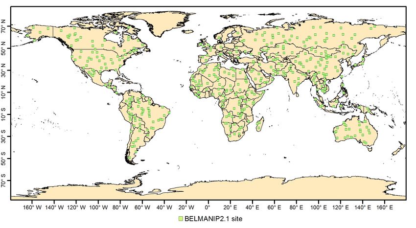
Remote Sens. 2018, 10, 1167                                                                          2 of 17

Index), FVC (Fraction Vegetation Cover) and FAPAR (Fraction of Absorbed Photosynthetically Active
Radiation) [3,4]. LAI accounts for the amount of green vegetation that absorbs or scatters solar
radiation, FVC determines the partition between soil and vegetation contributions, while FAPAR is
a vegetation health indicator related with ecosystems productivity. In addition, canopy water content
(CWC) accounts for the amount of water content at canopy level, varies with vegetation water status,
and is usually computed as the product of leaf water content (Cw ) and LAI [5,6]. These essential
variables can be estimated using remote sensing data and are key inputs in a wide range of ecological,
meteorological and agricultural applications and models.
     Biophysical variables can be derived from remote sensing data using statistical, physical and
hybrid retrieval methods [7–9]. Statistical methods rely on models to relate spectral data with the
biophysical variable of interest, usually through some form of regression. Statistical methods such
as neural networks [10], random forests [11] or kernel methods [12], extract patterns and trends
from a data set and approximate the underlying physical laws ruling the relationships between them
from data. Physically-based retrieval methods are based on the physical knowledge describing
the interactions between incoming radiation and vegetation through radiative transfer models
(RTMs) [13,14]. In particular, the MODIS LAI/FAPAR product is based on a three-dimensional RTM
which links surface spectral bi-directional reflectance factors (BRFs) to both canopy and soil spectral and
structural parameters [15]. On the other hand, hybrid methods couple statistical with physically-based
approaches inverting a database generated by an RTM [16–18]. For example, CYCLOPES global
products [19] were derived inverting the PROSAIL radiative transfer model [20] using neural networks,
while the global EUMETSAT LAI/FAPAR/FVC products are being produced inverting PROSAIL
with multi-output Gaussian process regression from the EUMETSAT Polar System (EPS) [21]. The use
of RTMs implies modeling leaf and canopy structural and biochemical parameters. The ranges and
distribution of parameters used for running the simulations are usually based on field measurements
that are very useful for simulating specific land covers [16,17]. Nevertheless, when the objective is
to simulate a wide range of vegetation situations and land covers, ground data is often a limitation.
In these scenarios, the scientific community uses distributions based on several experimental datasets
such as the HAWAII, ANGERS, CALMIT-1/2 and LOPEX [22–25] which together embrace hundreds
of observations [26]. Continuous update of ground measurements used for radiative transfer modeling
are key in order to better constrain the RTM inversion process [27]. In this framework, the use of global
plant traits database (TRY) [28] containing thousands of leaf data could alleviate this limitation.
     From an operational standpoint, processing remote sensing data on an ongoing basis demands
high storage capability and efficient computational power mainly when dealing with time series of long
term global data sets. This situation also occurs because of the wide variety of free available remote
sensing data disseminated by agencies such as the National Aeronautics and Space Administration
(NASA) (e.g., MODIS), the United States Geological Survey (USGS) (e.g., Landsat), and the European
Space Agency (ESA) (e.g., data from the Sentinel constellation) [29]. Recently, Google (Mountain View,
Cal., USA) developed the Google Earth Engine (GEE) [30], a cloud computing platform specifically
designed for geospatial analysis at the petabyte scale. The GEE data catalog is composed by widely
used geospatial data sets. The catalog is continuously updated and data are ingested from different
government-supported archives such as the Land Process Distributed Active Archive Center (LP
DAAC), the USGS, and the ESA Copernicus Open Access Hub. The GEE data catalogue contains
numerous remote sensing data sets such as top and bottom of atmosphere reflectance, as well
as atmospheric and meteorological data. Data processing is performed in a parallel on Google’s
computational infrastructure, dramatically improving processing efficiency, and opens up excellent
prospects especially for multitemporal and global studies that include vegetation, temperature, carbon
exchange, and hydrological processes [31–35].
     The present study proposes a generic retrieval chain for the production of global LAI, FAPAR, FVC
and CWC estimates from 15 years of MODIS data (MCD43A4) on the GEE platform. The methodology
Remote Sens. 2018, 10, 1167 3 of 17
is based on a hybrid method inverting a PROSAIL radiative transfer model database with random
forests (RFs) regression. Major contributions of the presented work are:
• The development of a general methodology for global LAI/FAPAR estimation including FVC and
CWC which are not provided by MODIS.
• The use of a global plant traits database (composed of thousands of data) for probability
density function (PDF) estimation with copulas to be used for radiative transfer modeling
leaf parameterization.
• The enforceability of biophysical parameter retrieval chain over GEE exploiting its capabilities to
provide climate data records of global biophysical variables at computationally both affordable
and efficient way.
Validation was performed by means of inter-comparison with the official MODIS LAI/FAPAR
product available on GEE (MCD15A3H) over a network of globally distributed sites. The only process
computed locally is the RTM simulation, while the inversion of the database, the derivation of the global
maps, and the assessment of the retrievals have been performed into the GEE platform. Furthermore,
the proposed methodology estimates both FVC and CWC variables which are not part of the official
MODIS products, giving an added value to this work.
The remainder of the paper is structured as follows. Section 2 describes the data used in this work
while Section 3 outlines the followed methodology. Section 4 exhibits the obtained results and the
validation of the global estimates, and Section 6 discusses the main conclusions of this work.
2. Data Collection
2.1. MODIS Data
In this study, we used the MCD43A4 and the MCD15A3H MODIS products both available in
GEE. Both the MCD (MODIS Combined Data) reflectance and LAI/FAPAR products are generated
combining data from Terra and Aqua spacecrafts and are disseminated in a level-3 gridded data
set. The MCD43A4 product provides a Bidirectional Reflectance Distribution Function (BRDF) from
a nadir view in the 1–7 MODIS bands (i.e., red, near infrared (NIR), blue, green, short wave infrared-1
(SWIR-1), short wave infrared-2 (SWIR-2), and middle wave infrared (MWIR), see Table 1). MCD43A4
offers global surface reflectance data at 500 m spatial resolution with 8-day temporal frequency.
Table 1. Spectral specifications of the MODIS MCD43A4 product.
MCD43A4 Band Wavelength (nm)
Band 1 (red) 620–670
Band 2 (NIR) 841–876
Band 3 (blue) 459–479
Band 4 (green) 545–565
Band 5 (SWIR-1) 1230–1250
Band 6 (SWIR-2) 1628–1652
Band 7 (MWIR) 2105–2155
On the other hand, GEE also offers access to MODIS derived LAI and FAPAR estimates through
the MCD15A3H collection 6 product. The temporal frequency of the biophysical estimates is every
four days, and the retrieval algorithm chooses the “best” pixel available from all the acquisitions of
both MODIS sensors from within the 4-day period. The MCD15A3H main retrieval algorithm uses
a look-up-table (LUT) approach simulated from a 3D RTM. Basically, this method searches for plausible
values of LAI and FAPAR for a specific set of angles (solar and view), observed bidirectional reflectance
factors at certain spectral bands, and biome types [15]. In addition, the MCD15A3H employs a back-up
algorithm (when the main one fails) that uses empirical relationships between NDVI (Normalized
Difference Vegetation Index) and the biophysical parameters. Similarly to MCD43A4, the pixel’s spatial
resolution is 500 m.Remote Sens. 2018, 10, 1167 4 of 17
2.2. Global Plant Traits
The TRY database represents the biggest global effort to compile a massive global repository
for plant trait data (6.9 million trait records for 148,000 plant taxa) at unprecedented spatial and
climatological coverage [28,36]. So far, the TRY initiative has delivered to the scientific community
around 390 million trait records which have resulted in more than 170 publications (https://www.
try-db.org/). The applications of the database range from functional and community ecology, plant
geography, species distribution, and vegetation models parameterizations [37–40].
We use a realistic representation of global leaf trait variability provided by the TRY to
optimize a vegetation radiative transfer model (PROSAIL), commonly used by the remote sensing
community [41]. Instead of using the common lookup tables available in the literature to parametrize
the model [19,21,42], we exploit the potential of the TRY database to infer the distributions and
correlations among some key leaf traits (leaf chlorophyll Cab , leaf dry matter Cdm and water Cw
contents) required by PROSAIL. Table 2 shows some basic information about the considered traits
extracted from the TRY.
Table 2. Information about the TRY data used in this work.
Trait Name Number of Samples Number of Species
Cab 19,222 941
Cdm 69,783 11,908
Cw 32,020 4802
3. Methodology
Physical approaches to retrieve biophysical variables rely on finding the best match between
measured and simulated spectra. The solution can be achieved by means of numerical optimization or
Monte Carlo approaches which are computationally expensive and do not guarantee the convergence
to an optimal solution. Recently, new and more efficient algorithms relying on Machine Learning
(ML) techniques have emerged and have become the preferred choice for most RTM inversion
applications [16–19,21]. In this work, we have followed the latter hybrid approach, combining radiative
transfer modeling and the parallelized machine learning RFs implementation available in GEE to
retrieve the selected biophysical variables. Figure 1 shows a schema of the work flow.
3.1. Creation of Leaf Plant Traits’ Distributions
Recent research has highlighted the importance of exploiting a priori knowledge to constrain
solutions of the ill-posed inversion problem in RTMs [27,43]. In this work, we used the TRY database
and the available literature to extract prior knowledge and improve our results. Despite using the
biggest plant trait database available, the representation of trait observations in a spatial and climate
context in the TRY is still limited, and it shows significant deviations among observed and modelled
distributions [28]. Trait measurements in the TRY represent the variation of single leaf measurements
because they are not abundance-weighted with respect to natural occurrence [28]. Trait distributions
are biased due to the availability of samples, which vary significantly due to technical difficulties for
sampling (e.g., very dense forests and remote areas) or the availability of funds to carry out expensive
field measurement campaigns in the different parts of the globe. To overcome these issues, we have
computed our leaf traits’ univariate distribution functions by combining the plant trait database (TRY)
with a global map of plant functional types (PFTs). The chosen global map of plant functional types
was the official MODIS (MCD12Q1) land cover product [44], we used this product to compute global
fractions of PFTs to weight more realistically species’ occurrence for the selected traits (leaf chlorophyll,
leaf dry matter, and leaf water contents).Remote Sens. 2018, 10, 1167 5 of 17
Figure 1. Work flow of the proposed retrieval chain over GEE.
The categorical information available in TRY allowed us to group leaf trait measurements in the
common PFT definitions. These grouped data were then used to compute individual normalized
histograms for each PFT, whereas the final leaf trait histogram was calculated as the weighted sum of
each PFT normalized histogram according to the global PFT’s spatial occurrence fractions. Repeating
this process for all considered leaf traits, we obtained their final univariate distribution functions.
These functions were inferred directly from the data by means of a non-parametric kernel density
estimation (KDE, [45]). This approach allowed us to model leaf probability distributions without
requiring any assumption regarding parametric families.
Some combinations of plant traits, like the ones considered in this work, exhibit significant
correlations and tradeoffs as a result of different plant ecological strategies [46]. In order to
capture these dependencies among traits, we created distributions that were also able to model
correlated multivariate data by means of different copula functions. These functions separate marginal
distributions from the dependency structure of a given multivariate distribution [47]. More precisely,
we use a multivariate Gaussian copula function [48]. Using the calculated marginal univariate
distributions for each trait and the Gaussian multivariate copula, computed from leaf measurements
of the TRY database, we created a set of random training samples while preserving the correlation
structure among them (see Figure 2).
Figure 2. Constrained random samples of leaf chlorophyll (Cab ), leaf dry matter (Cdm ), and leaf water
(Cw ) contents based upon prior knowledge of the TRY database, the MODIS land cover (MCD12Q1),
kernel density estimators, and copulas.Remote Sens. 2018, 10, 1167 6 of 17
3.2. Radiative Transfer Modeling
We used the PROSAIL RTM, which results from coupling the PROSPECT leaf optical model [49]
with the SAIL canopy reflectance model [50]. Note that we used the PROSPECT-5B [26] for the
coupling, which accounts for chlorophylls and carotenoids separately. PROSAIL was run in forward
mode for building a database mimicking MODIS canopy reflectance. These data were then used for
training the retrieval model assuming turbid medium canopies with randomly distributed leaves.
PROSAIL simulates top of canopy bidirectional reflectance from 400 to 2500 nm with a 1 nm spectral
resolution as a function of leaf biochemistry variables, canopy structure and background, as well as
the sun-view geometry. Leaf optical properties are given by the mesophyll structural parameter (N),
leaf chlorophyll (Cab ) and carotenoid (Car ) contents, leaf brown pigment (Cbp ) content, as well as leaf
dry matter (Cm ) and water (Cw ) contents. The average leaf angle inclination (ALA), the LAI, and the
hot-spot parameter (Hotspot) characterize the canopy structure. A multiplicative brightness parameter
(β s ) was used to represent different background reflectance types [19]. The system’s geometry was
described by the solar zenith angle, the view zenith angle, and the relative azimuth angle between
both angles, which in our case corresponded to illumination and observation zenith angles of 0◦ .
Sub-pixel mixed conditions (i.e., spatial heterogeneity) were tackled assuming a linear spectral mixing
model, which pixels are composed by a mixture of pure vegetation (vCover) and bare soil (1-vCover)
fractions’ [21].
The leaf variables were randomly generated following the calculated kernel density distributions
from the available leaf traits measurements, whereas distributions of the canopy variables as well as the
soil brightness parameter, were similar to those adopted in other global studies [19,21]. Brown pigments
were intentionally set to zero in order to account only for photosynthetic elements of the canopy (see
Table 3). In addition, with the aim of accounting for different sources of noise (e.g., atmospheric
correction, BRDF normalization or radiometric calibration) a wavelength dependent white Gaussian
noise was added to the reflectances of the PROSAIL simulations. Specifically, a Gaussian noise with
σ = 0.015 was added in the blue, green, and red channels, σ = 0.025 in the NIR, and σ = 0.03 in the
SWIR-1, SWIR-2 and MWIR.
Table 3. Distributions of the parameters within the PROSAIL RTM at leaf (PROSPECT-5B) and canopy
(SAIL) levels. * KDE refers to kernel density estimation method, which does not provide any parameters
being a non parametric model of the marginal distributions.
Parameter Min Max Mode Std Type
N 1.2 2.2 1.6 0.3 Gaussian
Cab (µg·cm−2 ) - - - - KDE *
Car (µg·cm−2 ) 0.6 16 5 7 Gaussian
Leaf
Cdm (g·cm−2 ) - - - - KDE *
Cw - - - - KDE *
Cbp 0 0 0 0 -
LAI (m2 /m2 ) 0 8 3.5 4 Gaussian
ALA (◦ ) 35 80 60 12 Gaussian
Canopy
Hotspot 0.1 0.5 0.2 0.2 Gaussian
vCover 0.3 1 0.99 0.2 Truncated Gaussian
Soil βs 0.1 1 0.8 0.6 Gaussian
3.3. Random Forests Regression
The inversion of PROSAIL was done using standard regression. There is a wide variety of
machine learning models for regression and function approximation. In this paper, we focus on the
particular family of methods called random forests (RFs). An RF is essentially an ensemble method
that constructs a multitude of decision trees (each of them trained with different subsets of features and
examples), and yields the mean prediction of the individual trees [51]. RFs’ classification and regressionRemote Sens. 2018, 10, 1167 7 of 17
have been applied in different areas of concern in forest ecology, such as modelling the gradient of
coniferous species [52], the occurrence of fire in Mediterranean regions [53], the classification of species
or land cover type [54,55], and the analysis of the relative importance of the proposed drivers [55] or
the selection of drivers [54,56,57]. The selection of RFs in our study is not incidental, and we capitalize
on several useful properties. The main advantage of using RFs over other traditional machine learning
algorithms like neural networks (NNETs) is that they can cope with high dimensional problems
very easily thanks to their pruning strategy. In addition, unlike kernel machines (KMs), RFs are
more computationally efficient. The RF strategy is very beneficial by alleviating the often reported
overfitting problem of simple decision trees. Moreover, this paper training data set has been split
into train and an independent test set that was only used for the assessment of the RFs. In addition,
RFs excel in the presence of missing entries, heterogeneous variables, and can be easily parallelized
to tackle large scale problems, which is especially relevant in the application described in this work.
This way, we can exploit large datasets and run predictions within Google Earth Engine easily. In this
work, we predicted the considered biophysical variables (LAI, FAPAR, FVC, and CWC) using the full
set of MODIS land bands shown in Table 1.
4. Results and Validation
4.1. Random Forests Theoretical Performance
In this section, we evaluate the RFs’ theoretical capabilities for LAI, FAPAR, FVC and CWC
retrieval. The training database was composed of 14,700 cases of reflectances in the MODIS channels
(Table 1) and the corresponding biophysical variables (i.e., LAI, FAPAR, FVC, and CWC) accounting
for any combination of the PROSAIL parameters. We first trained RFs with 70% of the PROSAIL
samples and then evaluated the estimation results over the remaining 30% of the samples (not in the
training). Figure 3 shows the scatter plots of the RFs’ estimates of every biophysical parameter over
the unseen test set. High correlations (R2 = 0.84, 0.89, 0.88, and 0.80 for LAI, FAPAR, FVC and CWC,
respectively) low Root-Mean-Squared Errors (RMSE = 0.91 m2 /m2 , 0.08, 0.06, and 0.27 kg/m2 for LAI,
FAPAR, FVC and CWC, respectively) and practically no biases were found in all cases (see Figure 3).
Figure 3. Theoretical performance of the Random forest regression over PROSAIL simulations of LAI,
FAPAR, FVC and CWC. The colorbar indicates density of points in the scatter plots.Remote Sens. 2018, 10, 1167 8 of 17
4.2. Obtained Estimates over GEE
After the RFs’ regression assessment undertaken in the previous section, we ran the retrieval
chain in GEE and obtained 15 years of global biophysical parameters. Here, we show the global mean
values of LAI, FAPAR, FVC and CWC derived from 2010 to 2015 (Figure 4). The spatial distribution
of retrieved parameters is expected, reaching the highest mean values close to the Equatorial zones
(Central Africa forests and Amazon basin) followed by the Northern latitudes (e.g., boreal forests).
In addition, Figure 5 shows the mean LAI and FAPAR values for the same period computed from the
GEE MODIS reference product (MOD15A3H) freely distributed from the Land Processes Distributed
Active Archive Center (LP DAAC) portal https://lpdaac.usgs.gov/.
Figure 4. LAI, FAPAR, FVC, and CWC global maps and latitudinal transects corresponding to the
mean values estimated by the proposed retrieval chain for the period 2010–2015.
Figure 5. LAI and FAPAR global maps and latitudinal transects corresponding to the mean values of
the GEE MODIS reference product (MOD15A3H) for the period 2010–2015.
4.3. Validation
Validation of LAI and FAPAR retrievals was undertaken by means of inter-comparison with
the available LAI/FAPAR product (MCD15A3H) on GEE. The inter-comparison was conducted over
a network of sites named BELMANIP-2.1 (Benchmark Land Multisite Analysis and Intercomparison
of Products). These sites were especially selected for representing the global variability of vegetation ,
making them suitable for global intercomparison of land biophysical products [58]. BELMANIP-2.1Remote Sens. 2018, 10, 1167 9 of 17
is an updated version of the original BELMANIP sites which includes 445 sites located in relatively
homogeneous areas all over the globe (see Figure 6). The sites are aimed to be representative of the
different planet biomes over an 10 × 10 km2 area, mostly flat, and with minimum fractions of urban
area and permanent water bodies.
Figure 6. Sites location of the BELMANIP-2.1 network used for intercomparison of LAI and FAPAR
retrievals and MOD15A3H LAI/FAPAR product.
We selected the MODIS pixels for every BELMANIP-2.1 location and then we computed the mean
value of the MODIS valid pixels within a 1 km surrounding area. We also considered the contribution
of partial boundary pixels by weighting their contribution to the mean according to their fractions
included within the selected area. Non-valid pixels (clouds, cloud shadows) and low-quality pixels
(back-up algorithm or fill values) were excluded according to the pixel-based quality flag in the MCD
products. In addition, since the MCD15A3H and MCD43A4 differ in temporal frequency, only the
coincident dates between them were selected for comparison. Due to the large amount of data available
in GEE, we were able to select only high-quality MODIS pixels, resulting in ∼60,000 valid pixels from
2002–2017 for validation. Figure 7 shows per biome scatter plots between the estimates provided by
the proposed retrieval chain and the reference MODIS LAI product over the BELMANIP2.1 sites from
2002 to 2012. Goodness of fit (R2 ) ranging from 0.70 to 0.86 and low errors (RMSE) ranging from 0.23
to 0.57 m2 /m2 are found between estimates in all biomes except for evergreen broadleaf forest, where
R2 = 0.42 and RMSE = 1.13 m2 /m2 are reported.
Similarly, Figure 8 shows the obtained scatter plots for FAPAR. In this case, very good agreement
(R2 ranging from 0.89 to 0.92) and low errors (RMSE ranging from 0.06 to 0.08) are found between
retrievals and the MODIS FAPAR product, over bare areas, shrublands, herbaceous, cultivated, and
broadleaf deciduous forest biomes. For needle-leaf and evergreen broadleaf forests lower correlations
(R2 = 0.57 and 0.41) and higher errors (RMSE = 0.18 and 0.09) are obtained. It is worth mentioning
that over bare areas, the MODIS FAPAR presents an unrealistic minimum value (∼0.05) through the
entire period.
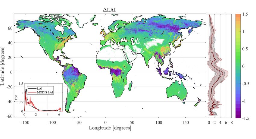
Figure 9 shows the LAI and FAPAR difference maps computed from the mean estimates
(2010–2015) provided by the proposed retrieval chain and the mean reference MODIS LAI/FAPAR
product. Mean LAI map revealed that most of the pixels fall within the range of ±0.5 m2 /m2 ,
which highlights the consistency between products. However, for high LAI values, there is an
underestimation of the provided estimates over very dense canopies that may reach up to 1.4 m2 /m2 .
In the case of FAPAR, there is a constant negative bias of ≈0.05 which is also noticeable in the scatter
plots shown in Figure 8. This is related with a documented systematic overestimation of MODIS FAPARRemote Sens. 2018, 10, 1167 10 of 17
retrievals [59–61], which is partly corrected by the proposed retrieval approach. The spatial consistency
of LAI/FAPAR estimates was also compared over the African continent (Figure 10). The latitudinal
transects provided by Figure 10 clearly show an underestimation of LAI retrievals in equatorial forests,
having a better agreement for the remaining biomes.
Figure 7. Biome-dependent scatter plots of the retrieved LAI over BELMANIP2.1 sites for the period
2002–2017. The colorbar indicates density of points in the scatter plots.Remote Sens. 2018, 10, 1167 11 of 17
Figure 8. Biome-dependent scatter plots of the retrieved FAPAR over BELMANIP2.1 sites for the
period 2002–2017. The colorbar indicates density of points in the scatter plots.Remote Sens. 2018, 10, 1167 12 of 17
Figure 9. LAI and FAPAR global maps and latitudinal transects corresponding to the difference of
mean values between derived estimates by the proposed retrieval chain and the GEE MODIS reference
product for the period 2010–2015.
Figure 10. LAI (left) and FAPAR (right) latitudinal profiles over Africa (longitude 22◦ E) corresponding
to the mean values of the GEE MODIS reference product and estimated by the proposed retrieval chain
for the period 2010–2015.
5. Discussion
The usefulness of GEE for providing global land surface variables related to vegetation status
was demonstrated in this work. GEE offers some major advantages mainly related to storage capacity
and processing speed. Despite the variety of algorithms implemented in GEE, its capabilities are
constrained by the number of state-of-the-art algorithms (in this case, regression-based) which are
currently implemented in GEE. However, this limitation is being overcome by the increasing number
of users developing algorithms that may be potentially implemented in GEE for a wide range of
applications. The functions in GEE utilize several built-in parallelization and data distribution models
to achieve high performance [30]. The RFs’ implementation in GEE is not an exception to that.
It allowed for the exploitation of large data sets and to obtain global estimates very efficiently. In GEE,
the system handles and hides nearly every aspect of how a computation is managed, including resource
allocation, parallelism, data distribution, and retries. These decisions are purely administrative; none
of them can affect the result of a query, only the speed at which it is produced [30]. Under these
circumstances, it is very difficult to give exact computation times because they vary in every run.
As an example, in the present work, to compute the mean biophysical maps implied to process 230
(46 yearly images × 5 years) FAPAR images at 500 m spatial resolution (∼440 million cells) and
compute their annual mean, it took around 6 h.Remote Sens. 2018, 10, 1167 13 of 17
The GEE data catalogue includes MODIS surface reflectance daily products, which can be
advantageous to fully exploit the information contained in the reflectance signal of the surface. In this
paper, we have preferred to use the normalized reflectance (MCD43A4) as an input. The BRDF
normalization and temporal compositing steps assume: (1) perfectness of the linear kernel model
inversion; (2) change of vegetation cover within temporal window is insignificant. These underlying
assumptions are approximate but allow robust estimates of the BRDF kernel coefficients. A number
of algorithms to retrieve satellite products (LAI, FAPAR and FVC) such as CYCLOPES (SPOT/VGT),
Copernicus (SPOT/VGT and PROBA-V), and LSA-SAF (MSG and EPS) use as input top of canopy
(TOC) normalized to a standard geometrical configuration [19,21,62]. This approach reduces
considerably the requirements in terms of number of inputs and computational load. Despite the
good speed potential of the proposed chain, the computational cost may be relevant when the aim
is to generate time series of global products. In order to reduce input uncertainties, we used the
quality flag provided by MCD43 products to filter non-valid pixels (persistent clouds and/or cloud
shadows in the MCD43 composite) as well as for identifying zones with low-quality pixels. Because
of the above-mentioned assumptions of the MCD43 product, further improvements of the proposed
methodology will include the uncertainty propagation of the reflectance input data to our retrievals
for operational use.
The comparison results between retrieved LAI/FAPAR and the reference MODIS product revealed
good spatial consistency. However, there are differences in mean LAI values over dense forests (up to
1.4 m2 /m2 ). The underestimation in high LAI values could be partly explained by two factors:
(1) differences in the algorithms used to estimate the LAI; and (2) the use of distinct LAI definitions for
each product estimates. Namely, the LAI retrieved by the proposed chain is based on the inversion of
a RTM assuming the canopy as a turbid medium. This approximation provides estimates closer to an
effective LAI (LAIe f f ). In turn, the MODIS retrieval algorithm accounts for vegetation clumping at leaf
and canopy scales through radiative transfer formulations, therefore estimated values should be closer
LAI
to actual LAI (LAIactual ). The relationship between LAIe f f and LAIactual is given by LAIactual Ωe f f
being Ω the cumpling index. Similar underestimation behaviour was found by other studies when
comparing MODIS LAI products and LAI retrievals from RTM inversion [59,63]. Yan et al. [59]
found RMSE = 0.66 m2 /m2 and RMSE = 0.77 m2 /m2 when comparing MODIS C6 LAI estimates with
ground LAIactual and LAIe f f measurements respectively, as well as larger uncertainties in high LAI
values. Regarding FAPAR, an overall negative bias is found for all biomes. However, this bias could
not be regarded as an issue in the estimations, since different studies have pointed out a systematic
overestimation of MODIS retrievals in both C5 and C6 at low FAPAR values as a main drawback of the
product [59–61]. For example, Xu et al. [64] assessed MODIS FAPAR through comparisons to ground
measurements available from 2012–2016, obtaining a reasonable agreement (R2 = 0.83, RMSE = 0.10)
but with an overall overestimation tendency (bias = 0.08, scatters distributed within 0–0.2 difference).
Similar results (R2 = 0.74, RMSE = 0.15) were reported by Yan et al. [59] using globally distributed
FAPAR measurements. The study evidenced a clear overestimation of FAPAR over sparsely-vegetated
areas, as noted previously in other studies [60].
It is worth mentioning that neither the FVC nor the CWC products are available on GEE. Moreover,
there is no global and reliable CWC product with which to compare the CWC estimates derived by the
proposed retrieval chain. Regarding FVC, there are only a few global products that differ in retrieval
approaches and spatiotemporal features. Since the main objective of the manuscript is to provide
a generic biophysical retrieval chain, including the validation with the corresponding biophysical
variables over GEE, the comparison of parameters not provided by GEE is out of the scope of the paper
and could be addressed in future works.
6. Conclusions
This paper proposed a processing chain for the estimation of global biophysical variables
(LAI, FAPAR, FVC, and CWC) from long-term (15-year) MODIS data in GEE. The approach takesRemote Sens. 2018, 10, 1167 14 of 17
the advantage of exploiting Earth observation data rapidly and efficiently through the GEE cloud
storage and parallel computing capabilities. The retrieval methodology is based on a hybrid approach
combining physically-based radiative transfer modelling (PROSAIL) and random forests regression.
The leaf parameter co-distributions employed during the radiative transfer modelling step were
obtained by means of exploiting the TRY database. This allowed a better PROSAIL parametrization
based on thousands of chlorophyll, water, and dry matter content ground measurements at leaf
level. The increasing amount of available plant trait data in TRY (containing thousands of records)
alleviates the need of a more realistic representation for some of the input parameters in radiative
transfer models.
A validation exercise was undertaken over the BELMANIP2.1 network of sites by means of
inter-comparison of the derived LAI and FAPAR with the MODIS reference LAI/FAPAR product
available on GEE. The obtained results highlight the consistency of the estimates provided by the
retrieval chain with the reference MODIS product. However, lower/poorer correlations were found
for evergreen broadleaf forests when compared with the rest of biomes. These discrepancies could
be mainly attributed to different retrieval approaches and variables definition, since derived LAI
estimates are closer to LAIe f f rather than LAIactual derived by the MOD15A3H product. In addition,
derived FAPAR stands only for photosynthetic elements of the canopy while FAPAR provided by
MODIS also accounts for non-photosynthetic elements. The proposed retrieval chain also derived
globally both FVC and CWC variables which are not provided by any GEE dataset.
The results demonstrated the usefulness of GEE for global biophysical parameter retrieval and
opened the door to user self-provisioning of leaf and canopy parameters in GEE for a wide range of
applications including data assimilation and sensor fusion.
Supplementary Materials: A toy example of the code is available at https://code.earthengine.google.com/
e3a2d589395e4118d97bae3e85d09106.
Author Contributions: All co-authors of this manuscript significantly contributed to all phases of the investigation.
They contributed equally to the preparation, analysis, review and editing of this manuscript.
Funding: The research leading to these results was funded by the European Research Council under Consolidator
Grant SEDAL ERC-2014-CoG 647423, the NASA Earth Observing System MODIS project (Grant NNX08AG87A),
and supported by the LSA SAF CDOP3 project, and the Spanish Ministry of Economy and Competitiveness
(MINECO) through the ESCENARIOS (CGL2016-75239-R) project.
Acknowledgments: The authors want to acknowledge the efforts of the TRY initiative on plant traits (http:
//www.try-db.org), hosted at the Max Planck Institute for Biogeochemistry, Jena, Germany.
Conflicts of Interest: The authors declare no conflict of interest.
References
1. Raich, J.W.; Schlesinger, W.H. The global carbon dioxide flux in soil respiration and its relationship to
vegetation and climate. Tellus B 1992, 44, 81–99. [CrossRef]
2. Beer, C.; Reichstein, M.; Tomelleri, E.; Ciais, P.; Jung, M.; Carvalhais, N.; Rödenbeck, C.; Arain, M.A.;
Baldocchi, D.; Bonan, G.B.; et al. Terrestrial Gross Carbon Dioxide Uptake: Global Distribution and
Covariation with Climate. Science 2010, 329, 834–838. [CrossRef] [PubMed]
3. Huete, A.; Didan, K.; Miura, T.; Rodriguez, E.P.; Gao, X.; Ferreira, L.G. Overview of the radiometric
and biophysical performance of the MODIS vegetation indices. Remote Sens. Environ. 2002, 83, 195–213.
[CrossRef]
4. Fensholt, R. Earth observation of vegetation status in the Sahelian and Sudanian West Africa: Comparison of
Terra MODIS and NOAA AVHRR satellite data. Int. J. Remote Sens. 2004, 25, 1641–1659. [CrossRef]
5. Clevers, J.G.P.W.; Kooistra, L.; Schaepman, M.E. Estimating canopy water content using hyperspectral
remote sensing data. Int. J. Appl. Earth Obs. Geoinf. 2010, 12, 119–125. [CrossRef]
6. Yebra, D.P.; Chuvieco, E.; Riaño, D.; Zylstra, P.; Hunt, R.; Danson, F.M.; Qi, Y.; Jurdao, S. A global review
of remote sensing of live fuel moisture content for fire danger assessment, moving towards operational
products. Remote Sens. Environ. 2013, 136, 455–468. [CrossRef]Remote Sens. 2018, 10, 1167 15 of 17
7. Wulder, M. Optical remote-sensing techniques for the assessment of forest inventory and biophysical
parameters. Prog. Phys. Geogr. 1998, 22, 449–476. [CrossRef]
8. Zheng, G.; Monika, M. Retrieving leaf area index (LAI) using remote sensing: theories, methods and sensors.
Sensors 1998, 9, 2719–2745. [CrossRef] [PubMed]
9. Verrelst, J.; Camps-Valls, G.; Muñoz-Marí, J.; Rivera, J.P.; Veroustraete, F.; Clevers, J.G.; Moreno, J.
Optical remote sensing and the retrieval of terrestrial vegetation bio-geophysical properties—A review.
ISPRS J. Photogramm. Remote Sens. 2015, 108, 273–290. [CrossRef]
10. Haykin, S. Neural Networks—A Comprehensive Foundation, 2nd ed.; Prentice Hall: Upper Saddle River, NJ,
USA, 1999.
11. Breiman, L. Random forests. Mach. Learn. 2001, 45, 5–32. [CrossRef]
12. Camps-Valls, G.; Bruzzone, L. Kernel Methods for Remote Sensing Data Analysis; Wiley & Sons: Chichester, UK,
2009; p. 434, ISBN 978-0-470-72211-4.
13. Myneni, R.B.; Ramakrishna, R.; Nemani, R.; Running, S.W. Estimation of global leaf area index and absorbed
PAR using radiative transfer models. IEEE Trans. Geosci. Remote Sens. 1997, 35, 1380–1393. [CrossRef]
14. Kimes, D.S.; Knyazikhin, Y.; Privette, J.L.; Abuelgasim, A.A.; Gao, F. Inversion methods for physically-based
models. Remote Sens. Rev. 2000, 18, 381–439. [CrossRef]
15. Knyazikhin, Y.; Glassy, J.; Privette, J.L.; Tian, Y.; Lotsch, A.; Zhang, Y.; Wang, Y.; Morisette, J.T.; Votava, P.;
Myneni, R.B.; et al. MODIS Leaf Area Index (LAI) and Fraction of Photosynthetically Active Radiation Absorbed
by Vegetation (FPAR) Product (MOD15) Algorithm Theoretical Basis Document; NASA Goddard Space Flight
Center: Greenbelt, MD, USA, 1999; Volume 20771.
16. Campos-Taberner, M.; García-Haro, F.J.; Camps-Valls, G.; Grau-Muedra, G.; Nutini, F.; Crema, A.;
Boschetti, M. Multitemporal and multiresolution leaf area index retrieval for operational local rice crop
monitoring. Remote Sens. Environ. 2016, 187, 102–118. [CrossRef]
17. Campos-Taberner, M.; García-Haro, F.J.; Camps-Valls, G.; Grau-Muedra, G.; Nutini, F.; Busetto, L.;
Katsantonis, D.; Stavrakoudis, D.; Minakou, C.; Gatti, L.; et al. Exploitation of SAR and Optical Sentinel
Data to Detect Rice Crop and Estimate Seasonal Dynamics of Leaf Area Index. Remote Sens. 2017, 9, 248.
[CrossRef]
18. Svendsen, D.H.; Martino, L.; Campos-Taberner, M.; García-Haro, F.J.; Camps-Valls, G. Joint Gaussian
Processes for Biophysical Parameter Retrieval. IEEE Trans. Geosci. Remote Sens. 2018, 56, 1718–1727.
[CrossRef]
19. Baret, F.; Hagolle, O.; Geiger, B.; Bicheron, P.; Miras, B.; Huc, M.; Berthelot, B.; Niño, F.; Weiss, M.;
Samain, O.; et al. LAI, fAPAR and fCover CYCLOPES global products derived from VEGETATION: Part 1:
Principles of the algorithm. Remote Sens. Environ. 2007, 110, 275–286. [CrossRef]
20. Baret, F.; Jacquemoud, S.; Guyot, G.; Leprieur, C. Modeled analysis of the biophysical nature of spectral
shifts and comparison with information content of broad bands. Remote Sens. Environ. 1992, 41, 133–142.
[CrossRef]
21. García-Haro, F.J.; Campos-Taberner, M.; Muñoz-Marí, J.; Laparra, V.; Camacho, F.; Sánchez-Zapero, J.;
Camps-Valls, G. Derivation of global vegetation biophysical parameters from EUMETSAT Polar System.
ISPRS J. Photogramm. Remote Sens. 2018, 139, 57–74. [CrossRef]
22. Jacquemound, S.; Bidel, L.; Francois, C.; Pavan, G. ANGERS Leaf Optical Properties Database (2003). Data
Set. Available online: http://ecosis.org (accessed on 5 June 2018).
23. Gitelson, A.A.; Merzlyak, M.N. Remote sensing of chlorophyll concentration in higher plant leaves.
Adv. Space Res. 1998, 22, 689–692. [CrossRef]
24. Gitelson, A.A; Buschmann, C.; Lichtenthaler, H.K. Leaf chlorophyll fluorescence corrected for re-absorption
by means of absorption and reflectance measurements. J. Plant Physiol. 1998, 152, 283–296. [CrossRef]
25. Hosgood, B.; Jacquemoud, S.; Andreoli, G.; Verdebout, J.; Pedrini, G.; Schmuck, G. Leaf Optical Properties
Experiment 93 (LOPEX93); European Commission—Joint Research Centre: Ispra, Italy, 1994; p. 20.
Available online: https://data.ecosis.org/dataset/13aef0ce-dd6f-4b35-91d9-28932e506c41/resource/
4029b5d3-2b84-46e3-8fd8-c801d86cf6f1/download/leaf-optical-properties-experiment-93-lopex93.pdf
(accessed on 5 June 2018).
26. Feret, J.B.; François, C.; Asner, G.P.; Gitelson, A.A.; Martin, R.E.; Bidel, L.P.R.; Ustin, S.L.; Le Maire, G.;
Jacquemoud, S. PROSPECT-4 and 5: Advances in the leaf optical properties model separating photosynthetic
pigments. Remote Sens. Environ. 2008, 112, 3030–3043. [CrossRef]Remote Sens. 2018, 10, 1167 16 of 17
27. Combal, B.; Baret, F.; Weiss, M.; Trubuil, A.; Mace, D.; Pragnere, A.; Myneni, R.B.; Knyazikhin, Y.; Wang, L.
Retrieval of canopy biophysical variables from bidirectional reflectance using prior information to solve the
ill-posed inverse problem. Remote Sens. Environ. 2002, 84, 1–15. [CrossRef]
28. Kattge, J.; Díaz, S.; Lavorel, S.; Prentice, I.C.; Leadley, P.; Bönisch, G.; Garnier, E.; Westoby, M.; Reich, P.B.;
Wright, I.J.; et al. TRY—A global database of plant traits. Glob. Chang. Biol. 2011, 17, 2905–2935. [CrossRef]
29. Wulder, M.A.; Coops, N.C. Make Earth observations open access: Freely available satellite imagery will
improve science and environmental-monitoring products. Nature 2014, 513, 30–32. [CrossRef] [PubMed]
30. Gorelick, N.; Hancher, M.; Dixon, M.; Ilyushchenko, S.; Thau, D.; Moore, R. Google Earth Engine:
Planetary-scale geospatial analysis for everyone. Remote Sens. Environ. 2017, 202, 18–27. [CrossRef]
31. Robinson, N.P.; Allread, B.W.; Jones, M.O.; Moreno, A.; Kimball, J.S.; Naugle, D.E.; Erickson, T.A.;
Richardson, A.D. A dynamic Landsat derived Normalized Difference Vegetation Index (NDVI) product for
the Conterminous United States. Remote Sens. 2017, 9, 863. [CrossRef]
32. Attermeyer, K.; Flury, S.; Jayakumar, R.; Fiener, P.; Steger, K.; Arya, V.; Wilken, F.; Van Geldern, R.; Premke, K.
Invasive floating macrophytes reduce greenhouse gas emissions from a small tropical lake. Sci. Rep. 2016,
6, 20424. [CrossRef] [PubMed]
33. Yu, M.; Gao, Q.; Gao, C.; Wang, C. Extent of night warming and spatially heterogeneous cloudiness
differentiate temporal trend of greenness in mountainous tropics in the new century. Sci. Rep. 2017, 7, 41256.
[CrossRef] [PubMed]
34. He, M.; Kimball, J.S.; Maneta, M.P.; Maxwell, B.D.; Moreno, A.; Begueria, S.; Wu, X. Regional Crop Gross
Primary Productivity and Yield Estimation Using Fused Landsat-MODIS Data. Remote Sens. 2018, 10, 372.
[CrossRef]
35. Kraaijenbrink, P.D.A.; Bierkens, M.F.P.; Lutz, A.F.; Immerzeel, W.W. Impact of a global temperature rise of
1.5 degrees Celsius on Asia’s glaciers. Nature 2017, 549, 257–260. [CrossRef] [PubMed]
36. Reichstein, M.; Bahn, M.; Mahecha, M.D.; Kattge, J.; Baldocchi, D.D. Linking plant and ecosystem functional
biogeography. Proc. Natl. Acad. Sci. USA 2014, 111, 13697–13702. [CrossRef] [PubMed]
37. Van Bodegom, P.M.; Douma, J.C.; Verheijen, L.M. A fully traits-based approach to modeling global vegetation
distribution. Proc. Natl. Acad. Sci. USA 2014, 111, 13733–13738. [CrossRef] [PubMed]
38. Madani, N.; Kimball, J.S.; Ballantyne, A.P.; Affleck, D.L.R.; Bodegom, P.M.; Reich, P.B.; Kattge, J.; Sala, A.;
Nazeri, M.; Jones, M.; et al. Future global productivity will be affected by plant trait response to climate.
Sci. Rep. 2018, 8, 2870. [CrossRef] [PubMed]
39. Wirth, C.; Lichstein, J.W. The Imprint of Species Turnover on Old-Growth Forest Carbon Balances-Insights
From a Trait-Based Model of Forest Dynamics. In Old-Growth Forests; Wirth, C., Heimann, M., Gleixner, G.,
Eds.; Springer: Jena, Germany, 2009; pp. 81–113, ISBN 978-3-540-92705-1.
40. Ziehn, T.; Kattge, J.; Knorr, W.; Scholze, M. Improving the predictability of global CO2 assimilation rates
under climate change. Geophys. Res. Lett. 2011, 38, 10. [CrossRef]
41. Berger, K.; Atzberger, C.; Danner, M.; D’Urso, G.; Mauser, W.; Vuolo, F.; Hank, T. Evaluation of the PROSAIL
Model Capabilities for Future Hyperspectral Model Environments: A Review Study. Remote Sens. 2018,
10, 85. [CrossRef]
42. Bacour, C.; Baret, F.; Béal, D.; Weiss, M.; Pavageau, K. Neural network estimation of LAI, fAPAR, fCover and
LAIxCab, from top of canopy MERIS reflectance data: Principles and validation. Remote Sens. Environ. 2014,
105, 313–325. [CrossRef]
43. Si, Y.; Schlerf, M.; Zurita-Milla, R.; Skidmore, A.; Wang, T. Mapping spatio-temporal variation of grassland
quantity and quality using MERIS data and the PROSAIL model. Remote Sens. Environ. 2012, 121, 415–425.
[CrossRef]
44. Friedl, M.A.; Sulla-Menashe, D.; Tan, B.; Schneider, A.; Ramankutty, N.; Sibley, A.; Huang, X. MODIS Collection
5 global land cover: Algorithm refinements and characterization of new datasets. Remote Sens. Environ. 2010,
114, 168–182. [CrossRef]
45. Parzen, E. On estimation of a probability density function and mode. Ann. Math. Stat. 1962, 33, 1065–1076.
[CrossRef]
46. Reich, P.B. The world-wide ‘fast–slow’ plant economics spectrum: A traits manifesto. J. Ecol. 2014, 102,
275–301. [CrossRef]
47. Nelsen, R.B. An Introduction to Copulass, 2nd ed.; Springer Science & Business Media: New York, NY, USA,
2009; ISBN 978-0387-28659-4.Remote Sens. 2018, 10, 1167 17 of 17
48. Žežula, I. On multivariate Gaussian copulas. J. Stat. Plan. Inference 2009, 111, 3942–3946. [CrossRef]
49. Jacquemoud, S.; Baret, F. PROSPECT: A model of leaf optical properties spectra. Remote Sens. Environ. 1990,
34, 75–191. [CrossRef]
50. Verhoef, W. Light scattering by leaf layers with application to canopy reflectance modeling: The SAIL model.
Remote Sens. Environ. 1984, 16, 125–141. [CrossRef]
51. Breiman, L.; Friedman, J.H. Estimating Optimal Transformations for Multiple Regression and Correlation.
J. Am. Stat. Assoc. 1985, 391, 1580–598.
52. Evans J.S.; Cushman, S.A. Gradient modeling of conifer species using random forests. Landsc. Ecol. 2009, 24,
673–683. [CrossRef]
53. Oliveira, S.; Oehler, F.; San-Miguel-Ayanz, J.; Camia, A.; Pereira, J.M.C. Modeling spatial patterns of fire
occurrence in Mediterranean Europe using Multiple Regression and Random Forest. For. Ecol. Manag. 2012,
275, 117–129. [CrossRef]
54. Gislason, P.O.; Benediktsson, J.A.; Sveinsson, J.R. Random Forests for land cover classification.
Pattern Recognit. Lett. 2006, 27, 294–300. [CrossRef]
55. Cutler, D.R.; Edwards, T.C.; Beard, K.H.; Cutler, A.; Hess, K.T.; Gibson, J.; Lawler, J.J. Random Forests for
classification in ecology. Ecology 2007, 88, 2783–2792. [CrossRef] [PubMed]
56. Genuer, R.; Poggi, J.M.; Tuleau-Malot, C. Variable selection using random forests. Pattern Recognit. Lett. 2010,
31, 2225–2236. [CrossRef]
57. Jung, M.; Zscheischler, J. A Guided Hybrid Genetic Algorithm for Feature Selection with Expensive Cost
Functions. Procedia Comput. Sci. 2013, 18, 2337–2346. [CrossRef]
58. Baret, F.; Morissette, J.T.; Fernandes, R.; Champeaux, J.L.; Myneni, R.B.; Chen, J.; Plummer, S; Weiss, M.;
Bacour, C.; Garrigues, S.; et al. Evaluation of the representativeness of networks of sites for the global
validation and intercomparison of land biophysical products: proposition of the CEOS-BELMANIP.
IEEE Trans. Geosci. Remote Sens. 2006, 44, 1794–1803. [CrossRef]
59. Yan, K.; Park, T.; Yan, G.; Liu, Z.; Yang, B.; Chen, C.; Nemani, R.R.; Knyazikhin, Y.; Myneni, R.B. Evaluation
of MODIS LAI/FPAR Product Collection 6. Part 2: Validation and Intercomparison. Remote Sens. 2016, 8, 460.
[CrossRef]
60. Camacho, F.; Cernicharo, J.; Lacaze, R.; Baret, F.; Weiss, M. GEOV1: LAI, FAPAR essential climate variables
and FCOVER global time series capitalizing over existing products. Part 2: Validation and intercomparison
with reference products. Remote Sens. Environ. 2013, 137, 310–329. [CrossRef]
61. Nestola, E.; Sánchez-Zapero, J.; Latorre, C.; Mazzenga, F.; Matteucci, G.; Calfapietra, C.; Camacho, F.
Validation of PROBA-V GEOV1 and MODIS C5 & C6 fAPAR Products in a Deciduous Beech Forest Site in
Italy. Remote Sens. 2017, 9, 126.
62. Baret, F.; Weiss, M.; Lacaze, R.; Camacho, F.; Makhmara, H.; Pacholcyzk, P.; Smets, B. GEOV1: LAI and
FAPAR essential climate variables and FCOVER global time series capitalizing over existing products. Part 1:
Principles of development and production. Remote Sens. Environ. 2013, 137, 299–309. [CrossRef]
63. Campos-Taberner, M.; García-Haro, F.J.; Busetto, L.; Ranghetti, L.; Martínez, B.; Gilabert, M.A.;
Camps-Valls, G.; Camacho, F.; Boschetti, M. A Critical Comparison of Remote Sensing Leaf Area Index
Estimates over Rice-Cultivated Areas: From Sentinel-2 and Landsat-7/8 to MODIS, GEOV1 and EUMETSAT
Polar System. Remote Sens. 2018, 10, 763. [CrossRef]
64. Xu, B.; Park, T.; Yan, K.; Chen, C.; Zeng, Y.; Song, W.; Yin, G.; Li, J.; Liu, Q.; Knyazikhin, Y.; et al. Analysis
of Global LAI/FPAR Products from VIIRS and MODIS Sensors for Spatio-Temporal Consistency and
Uncertainty from 2012–2016. Forests 2018, 9, 73. [CrossRef]
c 2018 by the authors. Licensee MDPI, Basel, Switzerland. This article is an open access
article distributed under the terms and conditions of the Creative Commons Attribution
(CC BY) license (http://creativecommons.org/licenses/by/4.0/).You can also read