Exploring the characteristics of a vehicle-based temperature dataset for convection-permitting numerical weather prediction
←
→
Page content transcription
If your browser does not render page correctly, please read the page content below
Exploring the characteristics of a vehicle-based temperature dataset
                                                       for convection-permitting numerical weather prediction

                                                 Authors: Zackary Bell1∗ , Sarah L. Dance1,2 and Joanne A. Waller3
                                                      1
                                                        Department of Meteorology, University of Reading, Reading, UK
                                                 2
                                                   Department of Mathematics and Statistics, University of Reading, Reading,
arXiv:2105.12526v1 [physics.ao-ph] 26 May 2021

                                                                                      UK
                                                          3
                                                            Met Office@Reading, University of Reading, Reading, UK
                                                                                            Abstract:
                                                       Crowdsourced vehicle-based observations have the potential to improve forecast skill in
                                                 convection-permitting numerical weather prediction (NWP). The aim of this paper is to explore
                                                 the characteristics of vehicle-based observations of air temperature. We describe a novel low-
                                                 precision vehicle-based observation dataset obtained from a Met Office proof-of-concept trial.
                                                 In this trial, observations of air temperature were obtained from built-in vehicle air-temperature
                                                 sensors, broadcast to an application on the participant’s smartphone and uploaded, with rele-
                                                 vant metadata, to the Met Office servers. We discuss the instrument and representation uncer-
                                                 tainties associated with vehicle-based observations and present a new quality-control procedure.
                                                 It is shown that, for some observations, location metadata may be inaccurate due to unsuitable
                                                 smartphone application settings. The characteristics of the data that passed quality-control
                                                 are examined through comparison with United Kingdom variable-resolution model data, road-
                                                 side weather information station observations, and Met Office integrated data archive system
                                                 observations. Our results show that the uncertainty associated with vehicle-based observation-
                                                 minus-model comparisons is likely to be weather-dependent and possibly vehicle-dependent.
                                                 Despite the low precision of the data, vehicle-based observations of air temperature could be a
                                                 useful source of spatially-dense and temporally-frequent observations for NWP.
                                                 Keywords: vehicle-based observations, road-surface energy balance, km-scale numerical
                                                 weather prediction, quality-control, crowdsourced data, dataset of opportunity
                                                 Correspondence: *Zackary Bell, Department of Meteorology, University of Reading, Earley
                                                 Gate, Whiteknights Road, Reading, RG6 6ET, United Kingdom, z.n.bell@pgr.reading.ac.uk
1 Introduction
Convection-permitting numerical weather prediction (NWP) requires a large number of ob-
servations of high spatio-temporal resolution to constrain short-term forecasts (Sun et al.,
2014; Gustafsson et al., 2018; Dance et al., 2019). However, due to the cost of installation,
management, and maintenance of observing instrumentation, it may be impractical to extend
traditional scientific observing networks to provide sufficient additional relevant observations.
A potential alternative source of inexpensive observations is from opportunistic data generated
by the public or other organisations (Waller, 2020; Blair et al., 2021).
The application of opportunistic datasets in NWP has been a popular area of research in recent
years (Hintz et al., 2019a). Observations from personal weather stations (PWSs) (Steeneveld
et al., 2011; Wolters and Brandsma, 2012; Chapman et al., 2017; Meier et al., 2017; Nipen
et al., 2020) and smartphones (Overeem et al., 2013; Droste et al., 2017; Madaus and Mass,
2017; Hintz et al., 2019b, 2020, 2021) are commonly obtained through crowdsourcing. Such ob-
servations may be inaccurate when compared with traditional scientific observations. However,
the number of crowdsourced observations available has the potential to far exceed the num-
ber of scientific surface observations currently produced (Muller et al., 2015). Opportunistic
datasets can also be obtained from partnerships with other organisations. For example, road-
side weather information station (RWIS) data obtained from highways agencies are currently
assimilated into the Met Office United Kingdom variable-resolution (UKV) model (Gustafsson
et al., 2018).
Observations obtained from vehicles are another dataset of opportunity (Mahoney and O’Sullivan,
2013). Similarly to PWS and smartphone observations, vehicle-based observations can be ob-
tained through crowdsourcing and will therefore be most densely distributed in urban areas
and on major transport networks. Vehicle-based observations can also be obtained through
several non-crowdsourcing methods. For example, the data can be obtained directly from vehi-
cle manufacturers through connected vehicle initiatives (e.g., Mahoney and O’Sullivan, 2013),
from built-in sensors of vehicle fleets via the controller area network (CAN) (e.g., Mercelis
et al., 2020), or through externally mounted sensors (e.g., Anderson et al., 2012). In this
paper, vehicle-based observations of air temperature are obtained from built-in vehicle sensors
through on-board diagnostic (OBD) dongles. This method of data collection, which is described
in section 3, could be used for crowdsourcing vehicle-based observations.
Vehicle-based observations are currently used to improve road weather modelling (e.g., Hu et al.,
2019) and forecasts to combat adverse road weather conditions on transportation networks (e.g.,
Karsisto and Nurmi, 2016; Siems-Anderson et al., 2019). Karsisto and Lovén (2019) showed
that assimilation of vehicle-based observations into the Finnish Meteorological Institute’s road
weather model had the greatest forecast impact factor when RWISs were sparse. The use of
vehicle-based observations in NWP is still in its infancy, but their use for nowcasting has been
investigated by the German weather service (DWD) (Hintz et al., 2019a). Additionally, an
observing simulation system experiment (OSSE) conducted by Siems-Anderson et al. (2020)
showed a modest but appreciable impact from assimilating simulated vehicle-based observa-
tions.
Before opportunistic datasets can be assimilated, they must undergo thorough quality-control
(QC) and the contributions to their observation uncertainty identified and investigated. Bell
et al. (2015) attributed the total uncertainty of crowdsourced PWS observations to five sources;
calibration issues, communication and software issues, inaccurate metadata, design flaws, and
error due to unresolved scales. As a result of these issues, which also apply to other opportunistic
datasets, the implementation of QC procedures can become substantially more difficult than
1the QC for traditional observations. In some studies over half the crowdsourced data were
removed by the QC procedure (e.g. Meier et al. (2017); Madaus and Mass (2017); Hintz
et al. (2019b)). Siems-Anderson et al. (2019) developed QC for vehicle-based observations
from disparate sources for use in road weather forecasting systems. However, these QC tests
required a large number of observations to be in close spatio-temporal proximity such that
spatial comparisons be used. Due to a lack of observations occurring at similar locations and
times for the dataset examined in this study, a new QC procedure was developed.
Understanding the characteristics of opportunistic observations is key to their effective use in
NWP (Waller, 2020). For data assimilation, an understanding of the instrument and repre-
sentation errors that contribute to the total observation uncertainty is required. Important
meteorological features such as sharp discontinuities caused by precipitation processes can be
observed by opportunistic observations but will likely be misrepresented by a NWP model
(Mahoney and O’Sullivan, 2013). Hence, it is likely that there will be significant represen-
tation error caused by the mis-match in scales observed and modelled (Janjić et al., 2018).
The instrument and representation components of the vehicle-based observation uncertainty
are discussed in section 2. For the vehicle-based observations of air temperature examined in
this study, an important physical feature misrepresented by a NWP model will be the under-
lying road surface. The influence of roads on the air temperature measured by vehicles will be
complex as the road-surface energy balance at a given location is substantially affected by the
availability of water, the quantity of visible sky, and the amount of traffic (e.g., Anandakumar,
1999; Chapman and Thornes, 2011; Oke et al., 2017; Karsisto and Lovén, 2019). To properly
understand the discrepancy between what is observed and modelled, it is necessary to examine
the characteristics of the differences between the model and the observations. The objective
of this paper is to explore the characteristics of a vehicle-based temperature dataset through
comparison with other datasets.
The format of this paper is as follows. In section 2 the uncertainties associated with vehicle-
based observations of air temperature are discussed. The Met Office trial used to obtain the
vehicle-based observations in this study, the datasets used for comparison, and the novel quality-
control procedure applied to the vehicle-based observations are detailed in section 3. The results
of the new quality-control process highlight that the observation location metadata can be in-
accurate due to poor GPS signal and application settings. A comparison between vehicle-based
observations and other datasets is given in section 4. Our novel results show that the uncer-
tainty of vehicle-based observations is likely weather-dependent and possibly vehicle-dependent.
In section 5 our results are summarised and we conclude that vehicle-based observations are a
promising opportunistic dataset for convection-permitting data assimilation.
2 Uncertainties in vehicle-based observations of air tem-
perature
2.1 Vehicle-based observations of air temperature from built-in sen-
sors
Most modern vehicles are equipped with a sensor to measure the air temperature of the sur-
rounding atmosphere. Throughout this paper, these sensors will be referred to as external
air-temperature sensors. Measurements obtained from external air-temperature sensors are
used by vehicle air conditioning systems to adjust cabin air temperature (Abdelhamid et al.,
2014) and alert the driver to safety hazards such as the possible presence of ice on the roads
(Padarthy and Heyns, 2019). External air-temperature sensors are commonly negative temper-
2ature coefficient thermistors (FierceElectronics, 2014). The location of external air-temperature
sensors will vary with vehicle make and manufacturer. Common placements are usually in the
airflow at the front of the vehicle, such as behind the grill near the bottom of the vehicle or in
the wing mirror (Tchir, 2016). We note that most vehicles also have a sensor that measures the
air temperature inside the vehicle engine commonly referred to as the intake air-temperature
sensor. These measurements, however, are contaminated with heat from the vehicle engine and
hence will not be representative of the true atmospheric conditions.
2.2 Instrument error
Built-in vehicle sensors are not intended to give high-quality meteorological information. As
such, observations of air temperature from external air-temperature sensors are likely to have
substantial instrument uncertainty. There are several sources of instrument uncertainty for
vehicle-based observations of air temperature:
1. The observations may be affected by extraneous influences (Mahoney and O’Sullivan,
2013).
2. The sensing instrument may not be as accurate or precise as required for meteorological
applications (Mahoney and O’Sullivan, 2013).
3. The ventilation of the sensing instrument may be inadequate (Harrison, 2015).
We now discuss these issues in more detail.
The extraneous influences that vehicle-based observations of air temperature are subject to
include heating from the vehicle engine or the underlying road surface. The degree of vehicle
influence on the observations will be determined by the sensors proximity to the vehicle engine.
Mercelis et al. (2020) found that observations of air temperature from external air-temperature
sensors situated far away from the vehicle engine were consistent with reliable observations
obtained from road weather information stations. In contrast, observations obtained from
sensors near the vehicle engine had to be discarded due to sensor biases. While external air-
temperature sensor placement is usually chosen to mitigate the influence of engine heat (Tchir,
2016), radiation reflected from the road surface can be incident on the sensor. Observations of
air temperature from external air-temperature sensors in such circumstances may be warmer
than the true ambient conditions.
The precision of an observation will depend on the number of significant figures available for
the digital representation of the measured value. (The concept we have called precision is
known in metrology as resolution (BIPM et al., 2012)). The difference between a continuous
variable and its imprecise digital representation is known as the quantization error (Widrow
et al., 1996). As the sensing instruments used for opportunistic datasets are not intended to
give high-quality meteorological information, quantization uncertainty will likely be part of the
instrument uncertainty (e.g., Mirza et al., 2016).
Adequate sensor ventilation is necessary to ensure accurate observations of air temperature
(Harrison and Burt, 2020). Sensor ventilation for external air-temperature sensors is determined
by how fast the vehicle is moving (e.g., Knight et al., 2010).
2.3 Representation error
Representation error is defined as the difference between a perfect observation and a model’s
representation of that observation (Janjić et al., 2018; Bell et al., 2020). The model’s represen-
tation of an observation is calculated using an observation operator. An observation operator
3is function that maps the model state into observation space. According to Janjić et al. (2018),
the representation error consists of three components:
1. The pre-processing error caused by the incorrect preparation of an observation.
2. The observation operator error due to any incorrect or approximate observation operators
used in the assimilation of an observation.
3. The error due to unresolved scales and processes when there is a mis-match in scales and
processes observed and modelled.
We now discuss these errors in more detail.
The pre-processing error for vehicle-based observations of air temperature can be caused by
the data collection and quality-control procedures. The height of external air-temperature
sensors will vary with vehicle type and sensor-height metadata will likely be unavailable in the
collection of crowdsourced datasets. Hence, the observations must be assigned a height which
may differ from the true height resulting in a height assignment error. The quality-control for
the vehicle-based observations is discussed in section 3.3.
Since air temperature is usually an NWP variable, the observation operator for vehicle-based
observations may be a simple interpolation operator. An observation operator error may result
from the misrepresentation of the vehicle-based observation height by the NWP model. The
resolution of NWP models is likely to be too coarse to represent the elevation of the vehicle-
based observations properly (Waller et al., 2021). This mismatch in elevation between a surface
observation and a NWP model field is normally accounted for by correcting the observation to
be at the same height as the model field. As air temperature is expected to change with altitude
in the surface layer (Stull, 1988a), the model height selected by the observation operator will
influence the value of the model-equivalent observation.
For vehicle-based observation of air temperature, errors due to unresolved scales and processes
are likely to be caused by deficiencies in the modelling of the local road-surface energy balance
(RSEB) between the net radiation into the road surface, the heating caused by traffic, the
ground heat flux density, the sensible heat flux density and the latent heat flux density (Karsisto
and Lovén, 2019). The amount of radiation absorbed by the road will vary across the road
due to the sky-view factor and traffic effects (Chapman and Thornes, 2011). The sky-view
factor indicates the amount of shielding from radiative heating and cooling and may be highly
spatially variable due to trees or buildings near the road. Chapman and Thornes (2011) showed
a rural example where the sky-view factor caused road-surface temperature to vary by almost
3◦ C. Traffic effects include the generation of turbulence by vehicles, friction heat dissipation
from tyres, sensible heat flux from vehicle engines, heat and moisture from exhaust fumes,
and the blocking of incoming solar radiation and outgoing longwave radiation from the road
surface (Prusa et al., 2002; Chapman and Thornes, 2005). Gustavsson et al. (2001) found that,
during morning commuting hours in urban areas, traffic caused the road surface temperature
to increase by approximately 2◦ C.
The materials used for road surfaces have a large heat capacity such that much of the radiation
absorbed by the surface is converted into ground heat flux (Anandakumar, 1999). The remain-
ing turbulent heat fluxes are determined by the amount of water available at the road surface
(Oke et al., 2017). If the road surface is dry, the remaining energy is entirely converted to sen-
sible heat, which will result in a strong vertical air-temperature gradient near the road surface.
Conversely, if water is available at the road surface, some of the remaining energy is converted
into latent heat and the air-temperature profile near the surface will be more uniform.
A common approach for modelling surface fluxes in NWP is through tile schemes (e.g., Essery
4et al., 2003). Using this approach, the surface flux of a grid box is the weighted average of
several different surface fluxes and hence may differ from the local RSEB substantially.
For road forecasting applications, outputs from NWP are post-processed in order to take better
account of the road physics (e.g., Clark, 1998; Coulson et al., 2012). For this initial study,
we do not use these post-processing techniques for simplicity. However, in principle, a more
sophisticated observation operator could use a similar approach to road forecasting models and
reduce the uncertainty due to unresolved scales.
3 Methodology
3.1 The Met Office trial
From 20th February 2018 to 30th April 2018 the Met Office ran a proof-of-concept trial to
collect vehicle-based observations of air temperature. The measuring instruments used in this
trial are those built-in by the manufacturer of the vehicle. In this trial, on-board diagnostic
(OBD) dongles were used to broadcast reports from the vehicle engine management interface
to an application (app) installed on a participant’s smartphone via Bluetooth. Additional
metadata derived from the smartphone was appended to the report, and uploaded to the Met
Office Weather Observations Website (Kirk et al., 2021) using the smartphone’s connection to
the mobile network (3G etc). A complete description of this trial can be found in Bell et al.
(2021). We now note some of the important aspects of the trial below.
The data collection frequency and GPS update period was set to 1 minute while the minimum
distance for a GPS update was set to 500 metres. We also note that a known fault that occurred
during this trial was for engine-intake temperature (i.e. the air temperature inside the vehicle
engine) to be recorded as air temperature for some observations. Observations were collected
throughout the United Kingdom with their locations corresponding to journeys undertaken by
the participants.
The dataset obtained through this trial consists of 67959 reports obtained from 31 Met Of-
fice volunteers. Each report contains some combination of observations of air temperature,
engine-intake temperature, and air pressure from built-in vehicle sensors. The observations of
temperature have a precision of 1◦ C while the observations of air pressure have a precision of
10hPa. We limit the scope of this study to air temperature only as engine-intake temperature
will not reflect the true atmospheric-air temperature and air pressure has too low precision to
be useful in NWP. The metadata for each report include vehicle speed (km/h), date-time (given
by the application as date and 24 hour clock time), GPS location, vehicle ID, and an unique
observation ID. With the exception of vehicle speed which was obtained by the OBD dongle,
all metadata was derived by the smartphone app.
3.2 Additional datasets used in this study
3.2.1 Met Office Integrated Data Archive System data
Met Office Integrated Data Archive System (MIDAS) temperature data consists of observa-
tions of 1.25m-air temperature which have a precision of 0.1◦ C and an uncertainty of 0.2◦ C
for various locations in the UK (Met Office, 2006). We use MIDAS daily maximum and mini-
mum temperature data in our quality-control procedure described in section 3.3. We also use
MIDAS hourly temperature data to provide a comparison with vehicle-based observations of
air temperature that are within 1.5km of a MIDAS station (see section 4.2). These data are
linearly interpolated to the time of a vehicle-based observation.
53.2.2 NWP model data
To explore the characteristics of the vehicle-based observations that pass quality-control we
use Met Office 10-minute UK variable-resolution (UKV) model data (Met Office, 2016). The
UKV is a variable resolution configuration of the Unified Model whose domain covers the
United Kingdom and Ireland (Lean et al., 2008). The inner domain has grid boxes of size
1.5km × 1.5km and fully covers the United Kingdom (Milan et al., 2020). Surrounding this is
a variable-resolution grid with boxes whose edges steadily increase in zonal and/or meridional
directions to 4km in size.
The UKV model fields we use in this study are 1.5m-air temperature and surface-air tem-
perature defined as the air temperature at the boundary with the surface. The UKV model
data are interpolated to the time and horizontal location of a vehicle-based observation so that
we can construct two observation-minus-background (OMB) datasets (i.e. one OMB dataset
using surface-air data for the background and another OMB dataset using 1.5m-air tempera-
ture for the background). Since a vehicle-based observation and the horizontally interpolated
background are both estimates of the true air temperature, their difference is equal to the
difference of their errors. If their errors are independent, the variance of their differences will
be equal to the sum of their individual error variances. Therefore, examining the statistics
of the two observation-minus-background datasets will provide insight into the uncertainty of
the vehicle-based observations. As the height of the external air-temperature sensor for each
vehicle is unknown, we are unable to interpolate the model data to the height of a vehicle-based
observation or correct the vehicle-based observation to be at the height of either UKV model
field. It is likely that the vehicle-based observations are between the two model heights and are
closer to the surface than the 1.5m height.
The surface flux for each grid box is determined by expressing the percentage of land use as a
combination of 5 vegetation and 4 non-vegetation tiles (Essery et al., 2003; Porson et al., 2010).
For each grid box, the surface flux is obtained by calculating the sum of the weighted average
of the fluxes from each tile (where instantaneous interaction between tiles is neglected). The
UKV uses the urban canopy model MORUSES (Met Office-Reading Urban Surface Exchange
Scheme) as the urban tile. MORUSES represents the impervious urban surface through a roof
tile and a canyon tile (Hertwig et al., 2020). However, observations taken on motorways and
major routes will often be surrounded by rural areas, and so the road fraction of the UKV grid
box will be small. For example, a typical UK motorway traversing a rural grid box occupies
less than 2% of the total area (Bremner, 2019).
3.2.3 Roadside weather information station observations
Vehicle-based observations of air temperature from built-in sensors are known to be consis-
tent with reliable observations obtained from roadside weather information stations (RWISs),
provided the external air-temperature sensor is located away from the engine block (Mercelis
et al., 2020). We therefore use RWIS data provided by Highways England (2018) to provide
a comparison with similar point observations for different weather conditions. There are over
250 RWISs in England located along major roads and major routes providing various roadside
meteorological information with a temporal frequency of 10 minutes (Buttell et al., 2020). In
this study, we use RWIS observations of air temperature that have precision of at least 0.1◦ C.
To give an indication of the total uncertainty of these observations, we note that the Met Office
currently assimilate RWIS observations of air temperature into the UKV with an uncertainty of
1◦ C. We note that the height that RWISs measure air temperature is estimated to be between
2 and 3 metres, but can be outside of this range if the site is located on a bank (Highways Eng-
land, 2020). Road-state classifiers (i.e. dry, trace amounts of water, wet) provided by RWISs
6are used to indicate the availability of water at the road surface. The RWIS observations are
linearly interpolated to the time that a vehicle passed a station.
3.3 Quality-control
In this section, we briefly describe the quality-control (QC) process applied to the vehicle-
based dataset. Further details are given by Bell et al. (2021). We note that, due to the size
and spatio-temporal sparsity of this dataset, we were unable to use spatial consistency QC
tests.
Before the QC process was implemented, an initial filtering of the raw data from the trial
was performed to ensure each observation had an air temperature observation and the relevant
metadata needed for each test. This filtering removed 35780 observations due to either a missing
air temperature observation or an invalid speed. The resultant dataset will be referred to as
the filtered dataset.
The QC process applied to the vehicle-based dataset began with three tests applied in parallel:
the climatological range test (CRT), the stuck instrument test (SIT), and the global positioning
system (GPS) test. Lastly, observations that passed each of these tests were then put through
a sensor ventilation test (SVT). The final quality-controlled dataset (QC-dataset) consisted of
all observations that passed the SVT. We now provide a brief description of each QC test.
The CRT checked if an observation was within a specified tolerance of a location-specific clima-
tology. For this dataset, we used MIDAS daily temperature data (Met Office, 2006) to create
monthly climatology datasets. These datasets were constructed by determining the maximum
and minimum air temperature of each MIDAS station active during February to April 2018
from pre-2018 data. The CRT was implemented by comparing the observation to the nearest
(in terms of great circle distance) MIDAS station monthly climatology dataset. If the obser-
vation was within a 2◦ C tolerance of the climatological range of the MIDAS station, then the
observation was passed.
The SIT examined portions of vehicle-specific time-series to check whether the vehicle sensor
was stuck on an air temperature value. This test required a vehicle identifier to determine
observations that came from the same source. (This may be unavailable in other crowdsourced
observation studies due to data privacy concerns). The SIT was implemented by comparing an
observation with all other observations from the same vehicle that occurred within a 15-minute
time-window. If there was at least one observation that had a different value of air temperature
to the tested observation, then the tested observation was passed. This test is essentially a
simplified version of a persistence test (see Zahumenskỳ (2004) for guidelines) that is able to
account for any short journeys undertaken by participants during the trial and the low precision
of the data.
The GPS test compared the location of an observation, denoted the test observation, relative
to a prior observation from the same vehicle, denoted the reference observation, to evaluate
the plausibility of the observation location metadata. The reference observation was at most
30 minutes before the test observation. As with the SIT, a vehicle identifier was required
to determine if observations came from the same source. The GPS test was implemented by
calculating the great-circle distance between the test and reference observations, dtest . Then
dtest was compared with the maximum and minimum distances estimated using the speed and
time metadata for the vehicle. The maximum distance was estimated by
demax = max(vtest , vref ) × ∆t, (3.1)
7QC test Number of tested Number of passed Number of flagged Number of untested
observations observations observations observations
Climatological range test 32179 32129 50 0
Stuck sensor test 32179 30124 2008 47
GPS test 32179 20162 11181 836
Sensor ventilation test 19094 17425 1669 0
Table 1: Summary of the results from all QC tests. The observations untested by the SIT and
GPS test are due to a lack of reference observations. The observations passed by the SVT form
the QC-dataset.
where vtest and vref are the speeds of the test and reference observations respectively, and ∆t
is the time-gap between the two observations. Similarly, the minimum distance was estimated
by
demin = min(vtest , vref ) × ∆t. (3.2)
The test observation passed the GPS test provided Γmin demin ≤ dtest ≤ Γmax demax where Γmin =
0.6 and Γmax = 1.3 are minimum and maximum multiplicative tolerance constants, respectively.
For justification of the choice of Γmin and Γmax , we refer the reader to Bell et al. (2021). Test
observations with ∆t < 1 minute or max(vtest , vref ) < 25km/h were passed if dtest ≤ Γmax demax
as they were expected to be close to the reference observation. (The specific choice of 25km/h
is related to the sensor ventilation test discussed in the next paragraph). If a test observation
did not have an observation from the same vehicle that occurred at most 30 minutes prior, then
it was left unclassified by the GPS test and became the reference observation for the next test
observation in the vehicle time-series.
The SVT was the final QC test which was applied to the observations that passed all previous
tests. This test involved checking that the speed metadata for each observation was above
a predetermined sensor ventilation threshold, vsensor . Examining the speed-temperature pairs
of the filtered dataset (not shown) revealed that the largest air temperatures (above 26◦ C)
occurred for speeds below 25km/h. We therefore set vsensor = 25km/h. An observation passed
the SVT if it had speed greater than vsensor . Hence, any observations that were passed by the
GPS test with low speeds were flagged by the SVT.
The QC-dataset contains 17425 observations (25.6% of original dataset). A summary of the
results of each QC test is provided in table 1. We note that the SIT and GPS test could not test
every observation in the filtered dataset due to unavailable or unsuitable reference observations.
The most discriminating test was the GPS test. The majority of observations flagged by the
GPS test were likely the result of the 500m update distance default setting on the app. We
also note that the SVT was a fairly discriminating test.
The QC approach taken with this dataset relied upon range validity and time-series tests.
For crowdsourced observations, time-series tests may be unsuitable as instrument identifica-
tion metadata may be unavailable due to data privacy concerns. This may be overcome with
appropriate encryption techniques (e.g., Verheul et al., 2019) or by performing the QC locally
on the sensing device (e.g., Hintz et al., 2019b). Furthermore, the use of spatial consistency
QC tests, which do not require instrument identification, would be a suitable replacement for
time-series-based tests provided there is a sufficient density of observations in a given area (e.g.,
Nipen et al., 2020).
84 Examination of the quality-controlled dataset
In this section we compare the QC-dataset with UKV model data, RWIS data, and MI-
DAS hourly data. Illustrative examples of the effect of sunny and rainy weather condi-
tions on vehicle-based observations are presented in section 4.1, analysis of observation-minus-
background (OMB) and observation-minus-observation (OMO) statistics are discussed in sec-
tion 4.2, and vehicle-specific OMB statistics are examined in section 4.3. We use UKV model
data as the background in the OMB datasets and MIDAS hourly data in the OMO dataset.
The effects of different meteorological factors are quantified through statistical analysis of OMB
departures grouped by sunny, cloudy and rainy weather conditions and season. The sunny
dataset will consist of observations that occur between 09:00 and 17:00 on days with at least
6 sunshine hours and less than 2mm of rainfall. Therefore, the observations are likely to be
influenced by solar radiation incident on UK roads. The rainy dataset will consist of observa-
tions that occur between 09:00 and 17:00 on days with at least 5mm of rainfall and less than
2 hours of sunshine. The cloudy dataset will consist of observations that occur between 09:00
and 17:00 on days with less 2 hours sunshine and 2mm rainfall. To obtain the weather-specific
sub-datasets, we used the Met Office daily weather summaries (Met Office, 2018). The seasons
we consider are Winter, defined as all data occurring between February 20th and March 20th
2018, and Spring, defined as all data occurring between March 21st and April 30th 2018. We
note that these seasons do not conform to the usual definitions of meteorological winter and
spring, but have been chosen due to the period of the Met Office trial and so that the Winter
and Spring datasets each contain a similar number of observations.
4.1 Case studies on the effect of sunny and rainy weather conditions
on vehicle-based observations
We now show three time-series of vehicle-based observations of air temperature, 10-minute UKV
1.5m-air-temperature and surface-air-temperature model data, and RWIS observations of air
temperature. The routes traversed in each time-series began and ended in suburban areas and
were predominantly on major roads and major routes in rural areas which occasionally crossed
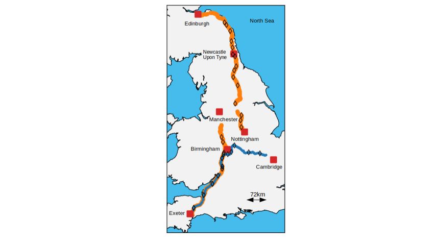
urban areas. The location of each time-series is shown in figure 1. We denote the time-series
shown in figure 2 as S1, figure 3 as S2, and figure 4 as R1. S1 and S2 are illustrative examples
of the effect of sunny weather and R1 is an illustrative example of the effect of rainy weather
on vehicle-based observations of air temperature. We note that the same vehicle produced the
observations in S1 and R1, but a different vehicle produced the observations in S2. We also
note that the large data gaps in the three time series are due to breaks in the journeys, and
the two small data gaps in S2 are due to observations removed by the QC procedure.
For clarity, we will refer to the OMB data using 1.5m-air temperature for the background as
aOMB and using surface-air temperature data for the background as sOMB. Furthermore, we
denote the bias (mean) and standard deviation of an aOMB dataset as µa and σa respectively
and the bias (mean) and standard deviation of a sOMB dataset as µs and σs respectively.
Figure 2 shows data from sunny weather conditions on March 25th 2018, including the time-
series S1, UKV and RWIS data. The OMB summary statistics for S1 are shown in table 2. The
sun rose at 06:52 and set at 18:22 on this day. The RWIS stations included in this time-series
recorded a dry road-state when the vehicle passed the station. As a result of these conditions,
we expect the sensible heat flux emitted by the road to be large and the road surface to have
a noticeable heating effect on the air temperature above (see section 2.3). Additionally, we
expect the surface-air temperature to be larger than the 1.5m-air temperature as the sensible
heat flux emitted by the UKV surface will also be large. The mean difference between the
9Figure 1: Map of the United Kingdom showing the location of the three time-series discussed in
section 4.1. The red squares show the location of cities passed by or near to the routes travelled
in the three time-series. The black diamonds show the location of the RWIS stations passed on
each journey. The two orange lines correspond to the sunny weather time-series and the blue
line corresponds to the rainy weather time-series. The time-series S1 began near Exeter and
travelled north towards Manchester. The time-series R1 travelled the same initial route as S1,
but headed east from Birmingham towards Cambridge. The time-series S2 began in Edinburgh
and travelled along the coast to Newcastle-upon-Tyne and then the vehicle travelled further
inland and south towards Nottingham.
Time-series
Summary Statistics S1 S2 R1
Number of observations 212 193 259
µa ◦ C 1.44 0.02 0.65
σa ◦ C 0.71 0.90 0.71
µs ◦ C −0.46 −0.27 0.37
σs ◦ C 1.21 1.71 0.64
Table 2: Summary of the OMB statistics for the three time-series shown in figure 1 using UKV
1.5m-air temperature and surface-air temperature as the background. The uncertainty in the
mean for each time-series is less than 0.1◦ C.
10Figure 2: Time-series S1 of 212 vehicle-based observations of air temperature (blue circles) from
a single vehicle driving along the M5 motorway on 25th March 2018 during sunny weather. Also
shown are UKV 1.5m-air temperature (purple triangles) and UKV surface-air temperature
(orange diamonds) linearly interpolated to the time and horizontal location of the vehicle
observations, and RWIS observations of air temperature (red squares) linearly interpolated to
the time the vehicle passed a station. The 1◦ C RWIS error bar represents the uncertainty used
to assimilate RWIS observations into the UKV.
interpolated RWIS observations and the nearest-in-time UKV model data reveals that RWIS
observations are in most agreement with 1.5m-air temperature and in least agreement with
surface-air temperature. There is a clear separation between UKV 1.5m-air temperature and
surface-air temperature at the start of the time-series that gradually decreases as the net ra-
diation absorbed by the UKV surface decreases. The vehicle-based observations generally lie
between the model fields as seen by the difference in sign between the biases, µa and µs . The
vehicle-based observations on average agree most with surface-air temperature as |µs | < |µa |.
This is consistent with the height of the vehicle sensor which is likely to be between the model
field heights of 0m and 1.5m but closer to 0m than 1.5m. Calculating the standard deviation
of the sOMB and aOMB departures shows that the sOMB departures are more variable as
σa < σs . We hypothesise that the variability of the UKV sensible heat flux induced by the
sunny weather conditions is the mechanism responsible for the larger sOMB variability.
Figure 3 shows data from sunny weather conditions on April 5th 2018, including the time-series
S2, UKV and RWIS data. The OMB summary statistics for S2 are shown in table 2. The sun
rose at 05:27 and set at 18:40 on this day. The RWISs included in this time-series recorded
a dry road-state when the vehicle passed the station. Similarly to the data in figure 2, the
RWIS observations are in most agreement with the UKV 1.5m-air temperature and in least
agreement with surface-air temperature. The surface-air temperature is larger than the 1.5m-
air temperature for the first half of this time-series. From approximately 17:00 we see that
1.5m-air temperature is greater than surface-air temperature. We hypothesise that this is due
to the stabilisation of the boundary layer (Stull, 1988b). In contrast to S1, the vehicle-based
observations are closest to UKV 1.5m-air temperature at the beginning of the time-series even
though the sensible heat flux emitted from the road surface is expected to be greatest during
this period. Possible reasons for this include cool breezes from the North Sea influencing the
11Figure 3: Time-series S2 of 193 vehicle-based observations of air temperature (blue circles) from
a single vehicle driving along the A1 and the M1 motorway on April 5th 2018 during sunny
weather. Also shown are UKV 1.5m-air temperature (purple triangles) and UKV surface-air
temperature (orange diamonds) interpolated to the time and horizontal location of the vehicle
observations, and RWIS observations of air temperature (red squares) interpolated to the time
the vehicle passed a station. The 1◦ C RWIS error bar represents the uncertainty used to
assimilate RWIS observations into the UKV.
vehicle-based observations during the beginning of the time-series (see route map in figure 1)
or because the air temperature is measured by a different vehicle’s instrument. Furthermore,
the difference between the biases µa and µs is large for S1 and small for S2. This, however, is
likely due to the large number of observations that occurred during the evening for S2 when
the temperature gradient between the surface and 1.5m is expected to be small. Considering
the observations from the first 3 hours of S2 only, when the net solar radiation absorbed by the
road and UKV surface is expected to be large, we find that the difference between the biases
µa and µs is more profound. We note that the standard deviations σa and σs are larger for
S2 than S1. This is likely due to the following two reasons. The first reason is the relatively
long temporal length of the S2 time-series. The second reason is the possible transition to
the nocturnal boundary layer as the dynamics induced by solar heating and the generation of
convective plumes begins to cease and surface layer starts to become stably stratified. However,
it is also plausible that the placement of the external air-temperature sensors on the two vehicles
is contributing to this behaviour.
Figure 4 shows data from rainy weather conditions on March 30th 2018, including the time-
series R1, UKV and RWIS data. The OMB summary statistics for R1 are shown in table
2. The RWIS stations included in this time-series recorded either a wet road-state or trace
amounts of water at the road surface when the vehicle passed the station. As a result of these
conditions, we expect the sensible heat emitted by the road to be small and the road surface to
have a reduced effect on the air temperature above (see section 2.3). We note that the drop in
air temperature between 12:30 and 13:30 is caused by an increase in altitude and an occluded
front. The mean difference between the interpolated RWIS observations and the nearest-in-
time UKV data reveals that RWIS observations are now in greater agreement with surface-air
temperature than 1.5m-air temperature. The two UKV model fields are similar throughout the
12Figure 4: Time-series R1 of 259 vehicle-based observations of air temperature (blue circles)
from a single vehicle driving along the M5 and M42 motorways and the A5 on 30th March 2018
during rainy weather conditions. Also shown are UKV 1.5m air temperature (purple triangles)
and UKV surface air temperature (orange diamonds) interpolated to the time and horizontal
location of the vehicle observations and RWIS observations of air temperature (red squares)
interpolated to the time the vehicle passed a station. The 1◦ C RWIS error bar represents the
uncertainty used to assimilate RWIS observations into the UKV.
time-series with multiple segments where the vehicle-based observations are greater than both
fields. The vehicle-based observations are on average greater than the UKV model data as the
biases µa , µs > 0◦ C but agree more with surface-air temperature as µa > µs . This indicates that
there are additional factors affecting the vehicle-based observations. Potential explanations for
this behaviour are given in section 4.2.4. We note that while the aOMB departures are more
variable than the sOMB departures (i.e. σa > σs ), they are similar in size.
The effect of the sensible heat emitted by the road and UKV surfaces can be observed through
comparison of the S1 and R1 time-series shown in figures 2 and 4, respectively. In sunny
weather, the sensible heat emitted by the road and UKV surface will be large, resulting in a
stronger vertical air-temperature gradient between the surface and the 1.5m height. In rainy
weather, the sensible heat emitted by the road and UKV surface will be small, leading to a
vertical air-temperature profile that is more uniform. Hence, the difference between the biases
µa and µs will be larger in sunny weather conditions than rainy weather conditions. The OMB
standard deviations calculated for each time-series show a negligible difference for σa and a
noticeable difference for σs between the two time-series. For the sOMB standard deviation σs ,
we see that it is smaller for rainy weather and larger for sunny weather. This is likely because
the variability of the sensible heat emitted by the UKV surface will be greater in sunny weather
than rainy weather. However, there may be other contributing factors such as the difference in
observation operator error between the two time-series.
134.2 Statistical analysis of observation-minus-background and observation-
minus-observation departures
In this section we investigate the uncertainty present in the QC-dataset through statistical
analysis of OMB and OMO departures. The OMB datasets will be partitioned into weather-
specific and seasonal sub-datasets so that we may examine how the OMB uncertainty changes
with weather conditions and season. As there are only 347 observations within 1.5km of a
MIDAS station, we will not split the OMO dataset into weather-specific and seasonal sub-
datasets. We now discuss the characteristics of each dataset.
4.2.1 QC-dataset OMB and OMO statistics
The OMB and OMO statistics corresponding to the QC-dataset are given in table 3. Examining
the OMB statistics shows that the vehicle-based observations are in poorer agreement with
1.5m-air temperature than surface-air temperature as the biases satisfy |µa | > |µs |. This
is expected as external air-temperature sensors likely measure air temperature nearer to the
surface than to a height of 1.5m. As µa > 0◦ C and µs > 0◦ C, vehicle-based observations
are on average warmer than both UKV model fields despite measuring the air temperature
between them. Possible reasons for this behaviour are discussed in section 4.2.4. For the
standard deviations, we have that σa < σs , showing that the sOMB dataset is more variable
than the aOMB dataset. This is also visible in the aOMB and sOMB distributions shown
by the histograms in figure 5a. While the distributions overlap substantially, a higher peak
is seen for the aOMB distribution, whereas the sOMB distribution has a larger left tail. It
is likely that the background uncertainty of surface-air temperature is greater than 1.5m-air
temperature due to the simplifying assumptions made by the UKV in modelling the SEB of a
grid box (see section 3.2.2).
Examining the OMO statistics reveals that vehicle-based observations are on average warmer
than MIDAS observations. Comparing the OMO departure bias, µm , with the biases µa and
µs obtained from the QC-dataset OMB departures, we find that µs < µm < µa . Hence, the
vehicle-based observations on average agree more with MIDAS data than 1.5m-air temperature
but still agree most with surface-air temperature. While it is plausible that vehicle-based
observations will generally agree more with MIDAS data than the UKV 1.5m-air temperature
model data, we note the following two issues with these calculations. Firstly, the MIDAS data
were not interpolated to the location of the vehicle-based observations and there will likely
be differences in elevation between the two. As air temperature is expected to change with
elevation in the surface layer (Stull, 1988a), the omission of any vertical interpolation may
cause a bias. Secondly, while the variability of the OMO dataset is less than the variability
of any OMB dataset shown in table 3, it is calculated with far fewer observations making the
statistic less reliable.
4.2.2 Weather-specific OMB datasets
The OMB statistics for each weather-specific dataset are given in table 3. For all weather
types, the bias µa is positive showing that vehicle-based observations are on average warmer
than UKV 1.5m-air temperature regardless of weather conditions. For the sunny and cloudy
datasets, the bias µs is negative, whereas for the rainy dataset µs is positive. This agrees
with the results of the three time-series discussed in section 4.1. This also suggests that the
vehicle-based observations studied in this paper may be colder on average than UKV surface-air
temperature in dry conditions. The smallest differences between the biases µa and µs occurs
for the rainy dataset while the largest difference occurs for the sunny dataset which is also seen
in the S1 and R1 time-series discussed in section 4.1. For the rainy dataset biases, we have that
14µa > 0◦ C and µs > 0◦ C which indicates the vehicle-based observations are on average warmer
than the two UKV model fields. This suggests that there are other influencing factors on the
vehicle-based observations that are not represented in the UKV as vehicles measure the air
temperature between these two heights. Potential explanations for this behaviour are discussed
in section 4.2.4.
Inspection of the weather-specific standard deviations reveals that, for sunny and cloudy
weather conditions, σs is noticeably larger than σa . This difference in variability is shown
in the histograms for the sunny dataset (figure 5b) and the cloudy dataset (figure 5c). The
sunny aOMB distribution is unimodal and the sunny sOMB distribution is bimodal. The bi-
modal structure may be due to intermittent cloud cover on the days with less sunshine hours or
the relatively small size of the sunny dataset. Similarly to the QC-dataset, the cloudy aOMB
and sOMB distributions overlap substantially, but a higher peak is seen for the aOMB distri-
bution and a larger left tail is seen for the sOMB distribution. For rainy weather conditions,
the standard deviations σa and σs are similar leading to similar aOMB and sOMB distributions
as shown in figure 5d.
Overall, the variability for the weather-specific datasets agrees with the variability calculated
for the time-series discussed in section 4.1. We also find that the standard deviation σs is larger
for the sunny sOMB dataset than for the cloudy sOMB dataset. This behaviour is likely the
result of the increased variability of the sensible heat emitted by roads and the UKV surface
during sunny weather conditions due to the larger amount of solar radiation absorbed by the
two surfaces. This also suggests that the uncertainty of vehicle-based observations may be
greatest in sunny weather conditions due to the combination of the radiative effects on the
vehicle sensor and the representation uncertainty. Conversely, the aOMB standard deviation
σa is largest for the cloudy dataset and not the sunny dataset. This, however, may be due to
changes in the sky-view factor due to variable cloud cover or because the cloudy dataset has
more observations than the sunny dataset. We hypothesise that the rainy dataset standard
deviations σs and σa are similar for the following three reasons. Rain increases the availability
of water at the UKV surface which reduces the emitted sensible heat flux and hence the vertical
air-temperature profile will be more uniform. There is also little to no sun at the times and
locations of the vehicle-based observations in the rainy dataset resulting in negligible radiation
reflected by the road surface incident on the vehicle temperature sensor. Finally, the rainy
dataset is the smallest of our three weather-specific datasets and so the OMB statistics are the
least robust.
4.2.3 Seasonal OMB datasets
The OMB statistics for the seasonal datasets are given in table 3 and the histograms are
plotted in figures 5e (Spring) and 5f (Winter). We include information on the seasonal datasets
to provide a baseline for the vehicle-specific analysis in section 4.3. For the seasonal datasets,
the vehicle-based observations are on average greater than the UKV model fields except for
surface-air temperature in Spring where they are approximately the same. Comparing the
biases of the seasonal datasets we see that µs is smaller and µa is greater in Spring than in
Winter. Inspection of the standard deviations of the seasonal datasets reveals that σs is larger
than σa in both Winter and Spring. Comparing the seasonal OMB statistics, we find that the
sOMB standard deviation σs is larger for the Spring dataset than for the Winter dataset. This
agrees with the results of the weather-specific datasets as the Spring dataset contains more
sunny days than the Winter dataset.
154.2.4 Discussion of the uncertainty exhibited by the OMB datasets
In this section we discuss several possible contributions to the uncertainty exhibited in the
OMB statistics shown in table 3.
• The vehicle-based observations of air temperature are precise to 1◦ C. The details of the
observation processing by the OBD system and app are unknown. However, an indication
of the expected size of the processing errors can be obtained by considering the quan-
tization error from a typical procedure thatprounds to the nearest integer. In this case,
the root-mean-squared quantization error is 1/12 ◦ C and may be a positive or negative
error (Widrow et al., 1996).
• As discussed in section 2.2, the external air-temperature sensors may exhibit a warm
bias from extraneous sources. For instance, the sensor may be in close proximity to the
vehicle engine or the location of the sensor may be inadequate for sensor ventilation. A
rough estimate of the bias due to the vicinity of the engine is 5◦ C - 25◦ C (Mercelis et al.,
2021). However there are several other factors that may be influencing this estimate (e.g.
differing vehicles).
• In unstable atmospheric conditions, the vertical air-temperature gradient between the
surface and the 1.5m height will be negative. When the sensible heat emitted by the road
and UKV surfaces is large, the vertical air-temperature gradient will be large. There-
fore, surface-air temperature will be warmer on average than vehicle-based observations
which likely measure air temperature between 20cm and 100cm above the road surface.
Similarly, 1.5m-air temperature will be cooler on average than vehicle-based observations.
• The vehicle-based observations have not been corrected to the elevation of the model grid
box. In NWP, it is common to correct surface observations using a standard adiabatic
lapse rate of 0.0065◦ C m−1 (Dutra et al., 2020; Cosgrove et al., 2003).
• The road surface temperature is highly variable due to sky-view factors and traffic (Chap-
man and Thornes, 2011). As noted in section 2.3, these factors can change the local
temperature by as much as 2 or 3◦ C.
• The difference in sensible heat emitted by the road surface and the UKV surface may
contribute to the OMB biases. As discussed in section 3.2.2, these model errors will vary
depending on the land-surface (e.g. urban/rural) but are difficult to quantify.
4.3 Vehicle specific observation-minus-background departure distri-
butions
Throughout the Met Office trial, 31 vehicles were used to produce vehicle-based observations.
To investigate whether error statistics differ with vehicle, we plot OMB histograms for each
of the 12 vehicles with the most observations between 09:00 and 17:00 in the QC-dataset in
figure 6. We use only observations between 09:00 and 17:00 so that the boundary layer is likely
to be unstable (i.e. UKV surface-air temperature is greater than the 1.5m-air temperature).
This is to avoid the complications of interpreting the OMB statistics experienced with the S2
time-series discussed in section 4.1 and so that more observations can be classified into the
weather-specific data types discussed in section 4.2. The OMB statistics are summarised in
table 4. Also included in table 4 is the percentage of observations for each vehicle occurring in
each weather-specific and seasonal dataset discussed in section 4.2. We note that it is difficult
to draw definitive conclusions in this examination for two reasons. Firstly, many of the vehicles
experience different weather conditions and there are many observations which we are unable
16(a) QC-dataset (b) Sunny dataset
(c) Cloudy dataset (d) Rainy dataset
(e) Spring dataset (f) Winter dataset
Figure 5: OMB histograms datasets corresponding to the datasets in table 3. Bins of width
0.5◦ C have been used for each histogram. The blue bars correspond to the aOMB bins and the
orange bars correspond to the sOMB bins.
17OMB and OMO statistics
Dataset Number of observations Departure Mean (◦ C) Standard deviation (◦ C)
aOMB 0.67 1.24
17425
QC-dataset sOMB 0.12 1.59
347 OMO 0.29 0.95
aOMB 1.05 1.15
Sunny 1878
sOMB −0.77 1.86
aOMB 0.84 1.41
Cloudy 2366
sOMB −0.14 1.74
aOMB 0.56 0.97
Rainy 840
sOMB 0.30 1.00
aOMB 0.48 1.29
Winter 7798
sOMB 0.26 1.55
aOMB 0.82 1.17
Spring 9627
sOMB 0.01 1.61
Table 3: Summary of the OMB and OMO departure statistics for each dataset. The uncertainty
in the mean for each dataset is less than 0.1◦ C.
to classify into a weather type. Secondly, there are only 12 vehicles with an acceptable number
of observations that we can examine.
The majority of histograms shown in figure 6 resemble normal distributions. The aOMB and
sOMB distributions of vehicles (ii), (iii), (iv), (x), and (xii) are qualitatively similar with the
visual distinction between them a result of the difference in means. The remaining vehicles
have noticeably different aOMB and sOMB distributions.
Examining the biases of the vehicle-specific OMB distributions shows that there are some
vehicles which agree more with UKV 1.5m air temperature than surface air temperature as
|µa | < |µs |. For these vehicles it is possible that the external air temperature sensor is located
closer to 1.5m height than the road surface or there are additional unknown factors affecting
the vehicle-based observations as in S2 discussed in section 4.1. The values of the biases µa
and µs also vary substantially between vehicles. The sign of µs also varies with vehicle whereas
only vehicle (x) has negative µa which suggests that some element of the vehicle’s external
air-temperature sensor or processing procedure may have a cold bias.
Except for vehicle (xii), we find that the aOMB dataset is less variable than the sOMB dataset
(i.e. σa < σs ) for all vehicles which agrees with the results obtained in sections 4.1 and 4.2.
The values of the standard deviations σa and σs also vary substantially between vehicles. When
stratifying the vehicles by seasonal contribution, we are able to find some agreement between
the OMB dataset variability. This can be seen between the groups of vehicles (ii) and (vii),
vehicles (iv), (viii) and (x), and vehicles (i) and (xi). Each vehicle in these groups contains
similar ratios of Winter to Spring observations. For vehicles (iii), (vi), (ix) and (xii), which
contain predominantly Spring observations, we see that the aOMB standard deviation σa is
similar except for vehicle (xii) and the sOMB standard deviation σs is similar except for vehicle
(iii). This shows that vehicles may have similar OMB uncertainty if they have similar ratios of
seasonal observations.
18You can also read