Crises and Recoveries in an Empirical Model of Consumption Disasters
←
→
Page content transcription
If your browser does not render page correctly, please read the page content below
American Economic Journal: Macroeconomics 2013, 5(3): 35–74
http://dx.doi.org/10.1257/mac.5.3.35
Crises and Recoveries in an Empirical Model of
Consumption Disasters†
By Emi Nakamura, Jón Steinsson, Robert Barro,
and José Ursúa*
We estimate an empirical model of consumption disasters using new
data on consumption for 24 countries over more than 100 years, and
study its implications for asset prices. The model allows for par-
tial recoveries after disasters that unfold over multiple years. We
find that roughly half of the drop in consumption due to disasters
is s ubsequently reversed. Our model generates a sizable equity pre-
mium from disaster risk, but one that is substantially smaller than
in simpler models. It implies that a large value of the intertemporal
elasticity of substitution is necessary to explain stock-market crashes
at the onset of disasters. (JEL E21, E32, E44, G12, G14)
T he average return on stocks is roughly 7 percent higher per year than the aver-
age return on bills across a large cross-section of countries in the twentieth
century (Barro and Ursúa 2008a). Mehra and Prescott (1985) argued that this large
equity premium is difficult to explain in simple consumption-based asset-pricing
models. A large subsequent literature in finance and macroeconomics has sought to
explain this “equity-premium puzzle.” In recent years, there has been growing inter-
est in the notion that the equity premium may be compensation for the risk of rare,
but disastrous, events such as wars, depressions, and financial crises (Rietz 1988;
Barro 2006).1
In Barro (2006), output is a random walk with drift, and rare disasters are identi-
fied as large, instantaneous, and permanent drops in output. He calibrates the fre-
quency and permanent impact of disasters to match large peak-to-trough drops in
real per capita GDP in a long-term panel dataset for 35 countries, and shows that his
model is able to match the observed equity premium with a coefficient of relative
risk aversion of the representative consumer of roughly 4. More recently, Barro and
*
Nakamura: Graduate School of Business, Columbia University, 3022 Broadway, New York, NY 10027 (e-mail:
enakamura@columbia.edu); Steinsson: Department of Economics, Columbia University, 420 W 118 St., New York,
NY 10027 (e-mail: jsteinsson@columbia.edu); Barro: Department of Economic, Harvard University, Littauer
Center, 1805 Cambridge St., Cambridge, MA 02138 (e-mail: rbarro@harvard.edu); Ursúa: Goldman Sachs, 200
West St., New York, NY 10282 (e-mail: jose.ursua@gs.com). We would like to thank Timothy Cogley, George
Constantinides, Xavier Gabaix, Ralph Koijen, Martin Lettau, Frank Schorfheide, Efthimios Tsionas, Alwyn Young,
Tao Zha, and seminar participants at various institutions for helpful comments and conversations. Barro would like
to thank the National Science Foundation for financial support through grant 0849496.
†
Go to http://dx.doi.org/10.1257/mac.5.3.35 to visit the article page for additional materials and author
disclosure statement(s) or to comment in the online discussion forum.
1
Piazzesi (2010) summarizes recent research on the equity premium, emphasizing four main explanations: hab-
its (Campbell and Cochrane 1999), heterogeneous agents (Constantinides and Duffie 1996), long-run risk (Bansal
and Yaron 2004), and rare disasters.
35
36 American Economic Journal: Macroeconomics July 2013
Ursúa (2008a) have gathered a long-term dataset for personal consumer expenditure
in over 20 countries and shown that the same conclusions hold using these data. A
growing literature has adopted this model and calibration of permanent, instanta-
neous disasters (e.g., Wachter forthcoming; Gabaix 2008; Farhi and Gabaix 2008;
Burnside et al. 2008; Guo 2007; and Gourio 2012).2
An important critique of the Rietz-Barro disasters model calibrated to match the
peak-to-trough drops in output or consumption is that it may overstate the riskiness
of consumption by failing to incorporate recoveries after disasters (Gourio 2008). A
world in which disasters are followed by periods of disproportionately high growth
is potentially far less risky than one in which all disasters are permanent. Kilian and
Ohanian (2002) emphasize the importance of allowing for large transitory fluctua-
tions associated with disasters, such as the Great Depression and WWII, in empirical
models of output dynamics. More generally, a large literature in macroeconomics has
debated whether it is appropriate to model output as trend or difference-stationary
(Cochrane 1988; Cogley 1990).
A second critique of the Rietz-Barro model is that it assumes that the entire drop
in output and consumption at the time of a disaster occurs instantaneously. In real-
ity, most disasters unfold over multiple years. This profile implies that even though
peak-to-trough declines in consumption exceeding 30 percent have occurred in
many countries, the annual decline in consumption in these episodes is considerably
smaller. Combining persistent declines in consumption into a single event might
not be an innocuous assumption. The assumption that the entire decline in output
and consumption associated with a disaster occurs in a single year is criticized in
Constantinides (2008). Similarly, Julliard and Ghosh (2012) argue that using annual
consumption data as opposed to peak-to-trough drops yields starkly different con-
clusions from Barro’s original calibration (Barro 2006).3
Given the growing importance of the disasters model in the macroeconomics,
international economics, and asset-pricing literatures, a key question is whether
it stands up to incorporating a more realistic process for consumption dynamics
during and following disasters. We develop a model of consumption disasters that
allows disasters to unfold over multiple years and to be systematically followed by
recoveries. The model also allows for transitory shocks to growth in normal times
and for a correlation in the timing of disasters across countries. This last feature
of the model allows us to capture the fact that major disasters, such as the world
wars of the twentieth century, affect many countries simultaneously. Ours is the first
paper to estimate the dynamic effects—both long term and short term—of these
major disasters on consumption.
2
Barro and Jin (2011) show that the required coefficient of relative risk aversion can be reduced to around three
if the size distribution of macroeconomic disasters is gauged by an estimated power-law distribution.
3
Julliard and Ghosh (2012) propose a novel approach to estimating the consumption Euler equation based on
generalized empirical likelihood methods, in the context of a representative agent consumption-based asset pricing
model with time-additive power utility preferences. A key difference between our framework and theirs is that they
focus on power utility, as in the original Rietz-Barro framework. We show that allowing for a more general prefer-
ence specification is crucial in assessing the asset pricing implications of multi-period disasters and recoveries.
Also, our approach does not rely on the exact timing of asset price returns during disasters. As we discuss below,
asset price returns during disasters play a disproportionate role in determining the equity premium; yet these are
also the periods for which asset price data are most likely to be either missing or inaccurate, for example, because
of price controls during wars.Vol. 5 No. 3 Nakamura et al.: Crises and Recoveries 37
We estimate our model on annual consumption data from the newly con-
structed Barro and Ursúa (2008a) dataset, using Bayesian Markov-Chain
Monte-Carlo (MCMC) methods.4 The model generates endogenous estimates of
the timing, magnitude, and length of disasters, as well as the extent of recovery
after disasters and the variance of shocks in disaster and nondisaster periods. Our
estimation procedure also allows us to investigate the statistical uncertainty associ-
ated with the predictions of the rare-disasters model along the lines suggested by
Geweke (2007) and Tsionas (2005).5
In estimating the model, we maintain the assumption that the frequency, size dis-
tribution, and persistence of disasters is time invariant and the same for all countries.
This strong assumption is important in that it allows us to pool information about
disasters over time and across countries. The rare nature of disasters makes it dif-
ficult to estimate accurately a model of disasters with much variation in structural
characteristics over time and space.
We find strong evidence for recoveries after disasters and for the notion that
disasters unfold over several years. We estimate that disasters last roughly six years,
on average. Over this period, consumption drops, on average, by about 30 percent
in the short run. However, about half of this drop in consumption is subsequently
reversed. The average long-run effect of disasters on consumption in our data is a
drop of about 15 percent.6 We find that uncertainty about future consumption growth
increases dramatically at the onset of a disaster. The standard deviation of consump-
tion growth in the disaster state is roughly 12 percent per year, several times its
value during normal times. The majority of the disasters we identify occur during
World War I, the Great Depression, and World War II. Other disasters include the
collapse of the Chilean economy, first in the 1970s and again in the early 1980s, and
the contraction in South Korea during the Asian financial crisis.
Our estimated model yields asset-pricing results that are intermediate between
models that ignore disaster risk and the more parsimonious disaster models con-
sidered in the previous literature. We adopt the representative-agent endowment-
economy approach to asset pricing—following Lucas (1978) and Mehra and
Prescott (1985)—and assume that agents have Epstein-Zin-Weil preferences. Our
model matches the observed equity premium with a coefficient of relative risk
aversion (CRRA) of 6.4 and an intertemporal elasticity of substitution (IES) of 2.
For these parameter values, a model without disasters yields an equity premium
only one-tenth as large, while a model with one-period, permanent disasters yields
an equity premium ten times larger. Given the close link between the equity pre-
mium and the welfare costs of economic fluctuations (Alvarez and Jermann 2004;
4
We use a Metropolized Gibbs sampler. This procedure is a Gibbs sampler with a small number of Metropolis
steps. See Gelfand (2000) and Smith and Gelfand (1992) for particularly lucid short descriptions of Bayesian esti-
mation methods. See, e.g., Gelman et al. (2004) and Geweke (2005) for comprehensive treatment of these methods.
5
In particular, we analyze the extent to which the observed asset returns are consistent with the posterior dis-
tribution of the equity premium implied by our model, taking into account parameter uncertainty. Tsionas (2005)
discusses in detail the importance of accounting for finite-sample biases and parameter uncertainty in assessing the
ability of alternative models to fit the observed equity premium, particularly in the presence of fat-tailed shocks.
6
Cerra and Saxena (2008) estimate the dynamics of GDP after financial crises, civil wars, and political shocks
using data from 1960 to 2001 for 190 countries. They find no recovery after financial crises, and political shocks but
partial recovery after civil wars. Their sample does not include World War I, the Great Depression, and World War
II. Davis and Weinstein (2002) document a large degree of recovery at the city level after large shocks.38 American Economic Journal: Macroeconomics July 2013
Barro 2009), these differences imply that our model yields costs of economic
fluctuations substantially larger than a model that ignores disaster risk, but substan-
tially smaller than the Rietz-Barro disaster model.
The differences between our model and the more parsimonious Rietz-Barro
framework arise both from the recoveries and the multi-period nature of disasters.
Recoveries imply that disasters have a much less persistent effect on dividends,
reducing the drop in stock prices when disasters occur. This modification, in turn,
lowers the equity premium. The multi-period nature of disasters affects the equity
premium in a more subtle way. To generate a high-equity premium, the marginal
utility of consumption must be high when the price of stocks drops. In our model,
the price of stocks crashes at the onset of disasters—with the initial news that a
disaster is underway—while consumption typically reaches its trough several years
later. This lack of coincidence between the stock market crash and the trough of
consumption reduces the equity premium in our model relative to the Rietz-Barro
model. In addition, since households anticipate persistent consumption declines at
the onset of a disaster—they expect things to get worse before they get better—they
have a strong motive to save that does not arise in the Rietz-Barro model. This
desire to save limits the magnitude of the stock market decline during disasters,
further reducing the equity premium. However, if agents have EZW preferences
with CRRA > 1 and IES > 1, the increase in uncertainty about future consumption
that occurs at the time of disasters raises marginal utility for a given value of current
consumption and, thus, increases the equity premium.
A key feature of our model is the predictability of consumption growth dur-
ing disasters—consumption typically declines for several years before recover-
ing. These features imply that the IES, which governs consumers’ willingness
to trade-off consumption over time, plays an important role in determining the
asset-pricing implications of our framework. There is considerable debate in
the macroeconomics and finance literature about the value of the IES. Several
authors—notably Hall (1988)—argue that the IES is close to zero. However, oth-
ers, such as Bansal and Yaron (2004) and Gruber (2006), argue for substantially
higher values of the IES.
The large movements in expected consumption growth associated with disasters
provide a strong test of consumers’ willingness to substitute consumption over time.
For a low value of the IES, our model implies a surge in stock prices at the onset of
disasters and a negative equity premium in normal times. The reason is that entering
the disaster state generates a strong desire to save, because consumption is expected
to fall further in the short run. When the IES is substantially below one, this savings
effect dominates the negative effect that the disaster has on expected future divi-
dends from stocks and, therefore, raises the price of stocks.7 These predictions do
not accord with the available evidence. Disasters are typically associated with stock
market crashes. This observation supports the view that consumers have a relatively
high willingness to substitute consumption over time (at least during disasters),
motivating a high value of the IES.
7
Gourio (2008) makes this point forcefully in a simpler setting. For similar reasons, an IES larger than one
plays an important role in the long-run risk model of Bansal and Yaron (2004).Vol. 5 No. 3 Nakamura et al.: Crises and Recoveries 39
Our estimated model yields additional predictions for the behavior of short-term
and long-term interest rates. One potential concern is that the same factors driving a
high equity premium would also generate a high term premium—a prediction that is
not supported by the empirical evidence (Campbell 2003; Barro and Ursúa 2008a).
We show that this is not the case. Our model implies a positive equity premium but
a negative term premium for risk-free long-term (real) bonds that arises from the
hedging properties of long-term bonds during disaster periods. Our model also gen-
erates new predictions for the dynamics of risk-free interest rates surrounding disas-
ters. In particular, the strong desire to save during disasters drives down the return
on short-term bonds, leading to low real interest rates during disaster episodes, as
observed in the data.
We consider an extension of our model that allows for partial default on bonds.
Empirically, inflation risk is an important source of partial default on govern-
ment bonds. Data on stock and bond returns over disaster periods indicate that
short-term bonds provide substantial insurance against disaster risk in only
about 70 percent of cases. When we allow for an empirically realistic degree of
default on short-term bonds, a risk aversion parameter of 7.5 is needed to fit the
observed equity premium. Because inflation unfolds sluggishly in the data, the
effect of inflation risk on short-term bonds is less severe than on long-term bonds.
Incorporating this fact allows us to match the upward-sloping term premium for
nominal bonds.
We employ the Mehra and Prescott (1985) methodology for assessing the asset-
pricing implications of our model. Hansen and Singleton (1982) pioneered an
alternative methodology based on measuring the empirical correlation between
asset returns and the stochastic discount factor. An important difficulty with
employing the Hansen-Singleton approach is that the observed timing of real
returns on stocks and bonds relative to drops in consumption during disasters is
affected by gaps in the data on asset prices, as well as price controls, asset price
controls, and market closure. For example, stock price data are missing for Mexico
in 1915–1918, Austria in World War II, Belgium in World War I and World War
II, Portugal in 1974–1977, and Spain in 1936–1940. The Nazi regime in Germany
imposed price controls in 1936 and asset-price controls in 1943 that lapsed only in
1948. In France, the stock market closed in 1940–1941 and price controls affected
measured real returns over a longer period. Given these data limitations, Barro and
Ursúa (2009a) take the approach of computing the covariance between the peak-
to-trough decline in asset prices and a consumption-based stochastic discount fac-
tor using a “flexible timing” assumption regarding the intervals over which these
declines occur. Under this assumption, it is possible to match the equity premium
for moderate values of risk aversion. Their calculations highlight the dispropor-
tionate importance of disasters in matching the equity premium. Nondisaster
periods contribute trivially to the equity premium.8
8
Another concern regarding the Hansen-Singleton methodology, emphasized by Geweke (2007) and Arakelian
and Tsionas (2009), is that parsimonious asset pricing models are sufficiently stylized so that formal statistical
rejections may not be very informative.40 American Economic Journal: Macroeconomics July 2013
A number of recent papers study whether the presence of rare disasters may also
help to explain other anomalous features of asset returns, such as the predictabil-
ity and volatility of stock returns. These papers include Farhi and Gabaix (2008),
Gabaix (2008), Gourio (2008), and Wachter (forthcoming). Martin (2008) presents
a tractable framework for asset pricing in models of rare disasters. Gourio (2012)
embeds disaster risk in a b usiness-cycle model and shows that time-varying disaster
risk can generate joint dynamics of macroeconomic aggregates and asset prices that
are consistent with the data.
The paper proceeds as follows. Section I discusses the Barro-Ursúa data on long-
term personal consumer expenditures. Section II presents the empirical model.
Section III discusses our estimation strategy. Section IV presents our empirical esti-
mates. Section V studies the asset-pricing implications of our model. Section VI
concludes.
I. Data
In estimating our disaster model, it is crucial to use long time series whose start-
ing and ending points are not endogenous to the disasters themselves. It is also
crucial that the dataset contain information on the evolution of macroeconomic vari-
ables during disasters; Maddison’s (2003) tendency to interpolate GDP data during
wars and other crises is not satisfactory for our purposes. Furthermore, to analyze
the asset-pricing implications of rare disasters, it is important to measure consump-
tion dynamics, as opposed to output dynamics.
We use a recently created dataset on long-term personal consumer expenditures
constructed by Barro and Ursúa and described in detail in Barro and Ursúa (2008a).9
This dataset includes a country only if uninterrupted annual data are available back
at least before World War I, yielding a sample of 17 Organisation for Economic
Co-operation and Development (OECD) countries and 7 non-OECD countries.10
To avoid sample selection bias problems associated with the starting dates of the
series, we include only data after 1890. The resulting dataset is an unbalanced panel
of annual data for 24 countries, with data from each country starting between 1890
and 1914 and ending in 2006, yielding a total of 2,685 observations.
One limitation of the Barro-Ursúa consumption dataset is that it does not allow
us to distinguish between expenditures on nondurables and services versus durables.
Unfortunately, separate data on durable and nondurable consumption are not avail-
able for most of the countries and time periods we study. For time periods when
such data are available, however, the effect of excluding durables on the overall
decline in consumer spending during disasters is small. The proportionate decline
in spending on nondurables and services is, on average, only 3 percentage points
9
These data are available from Barro’s website, at: http://www.economics.harvard.edu/faculty/barro/data_
sets_barro.
10
The OECD countries are: Australia, Belgium, Canada, Denmark, Finland, France, Germany, Italy, Japan,
Netherlands, Norway, Portugal, Spain, Sweden, Switzerland, the United Kingdom, and the United States. The
“non-OECD” countries are Argentina, Brazil, Chile, Mexico, Peru, South Korea, and Taiwan. See Barro and
Ursúa (2008a) for a detailed description of the available data and the countries dropped due to missing data. In
cases where there is a change in borders, as in the case of the unification of East and West Germany, Barro, and
Ursúa (2008a) smoothly paste together the initial per capita series for one country with that for the unified country.Vol. 5 No. 3 Nakamura et al.: Crises and Recoveries 41
smaller than the overall decline in consumer spending (Barro and Ursúa 2008a).
The reason is that for most of the time period we study, durables accounted for only
a small fraction of consumer expenditures. The effect of excluding durables is even
smaller during the largest disasters, because durable consumer expenditures can at
most fall to zero. The remaining fall in consumer expenditures must come entirely
from nondurable expenditures.
In analyzing the asset-pricing implications of our model, we make use of total
returns data on stocks, bills, and bonds from Global Financial Data (GFD), aug-
mented with data from Dimson, Marsh, and Staunton (2002) and other sources.
These data are described in detail in Barro and Ursúa (2009a). Unfortunately,
these data are less comprehensive than the corresponding consumption series and
often contain gaps for disaster periods. Price controls and controls on asset prices
also make the exact timing of real returns difficult to measure during disasters.
We therefore use these data to assess the predictions of our model primarily by
considering average returns in nondisaster periods and cumulative returns over
disaster periods.
II. An Empirical Model of Consumption Disasters
We model log consumption as the sum of three unobserved components:
(1) ci, t = xi, t + zi, t + ϵi, t ,
where c i, t denotes log consumption in country i at time t, x i, t denotes “potential”
consumption in country i at time t; zi, tdenotes the “disaster gap” of country i at time
t—i.e., the amount by which consumption differs from potential due to current and
past disasters; and ϵi, t denotes an independently and identically disributed normal
shock to log consumption with a country-specific variance σ 2ϵ, i, tthat potentially var-
ies with time.
The occurrence of disasters in each country is governed by a Markov process Ii, t .
Let Ii, t= 0 denote “normal times” and I i, t= 1 denote times of disaster. The probabil-
ity that a country that is not in the midst of a disaster will enter the disaster state is
made up of two components: a world component and an idiosyncratic component.
Let I W , tbe an independently and identically distributed indicator variable that takes
the value IW, t= 1 with probability pW. We will refer to periods in which IW, t= 1 as
periods in which “world disasters” begin. The probability that a country not in a
disaster in period t − 1 will enter the disaster state in period t is given by pCbW IW, t +
pCbI (1 − IW, t), where p CbW is the probability that a particular country will enter a
disaster when a world disaster begins, and pC bI is the probability that a particular
country will enter a disaster “on its own.” Allowing for correlation in the timing of
disasters through I W, tis important for accurately assessing the statistical uncertainty
associated with the probability of entering the disaster state. Once a country is in a
disaster, the probability that it will exit the disaster state each period is pC e.
We model disasters as affecting consumption in two ways. First, disasters cause
a large short-run drop in consumption. Second, disasters may affect the level of42 American Economic Journal: Macroeconomics July 2013
p otential consumption to which the level of actual consumption will return. We
model these two effects separately. First, let θi, tdenote a one-off permanent shift in
the level of potential consumption due to a disaster in country i at time t. Second,
let ϕi, tdenote a shock that causes a temporary drop in consumption due to the disas-
ter in country i at time t. For simplicity, we assume that θ i, t does not affect actual
consumption on impact, while ϕ i, t does not affect consumption in the long run.
In this case, θi, t may represent a permanent loss of time spent on R&D and other
activities that increase potential consumption or a change in institutions that the
disaster induces. The short-run shock, ϕ i, t , could represent destruction of structures,
crowding out of consumption by government spending, and temporary weakness of
the financial system during the disaster.
We assume that θ i, t is distributed θi, t ∼ N(θ, σ 2θ ). This implies that we do not
rule out the possibility that disasters can have positive long-run effects. Crises
can, e.g., lead to structural change that benefits the country in the long run. We
consider two distributional assumptions for the short-run shock ϕi, t . Both of these
distributions are one-sided, reflecting our interest in modeling disasters. In our
baseline case, ϕ i, thas a truncated normal distribution on the interval [−∞, 0]. We
denote this as ϕ i, t ∼ tN(ϕ∗, σ ∗2
ϕ , −∞, 0), where ϕ ∗and σ ∗2
ϕ denote the mean and
variance, respectively, of the underlying normal distribution (before truncation).
We use ϕ and σ 2ϕ to denote the mean and variance of the truncated distribution.
We also estimate a model with −ϕi, t ∼ Gamma(αϕ , βϕ). The gamma distribution
is a flexible one-sided distribution that has excess kurtosis relative to the normal
distribution.
Potential consumption evolves according to
(2) xi, t = μi, t + ηi, t + Ii, t θi, t ,
Δ
where Δ denotes a first difference, μ i, t is a country-specific average growth rate of
trend consumption that may vary over time, ηi, tis an independently and identically
distributed normal shock to the growth rate of trend consumption with a country
2η, i . This process for potential consumption is similar to the pro-
specific variance σ
cess assumed by Barro (2006) for actual consumption. Notice that consumption in
our model is trend stationary if the variances of ηi, tand θi, tare zero.
The disaster gap follows an AR(1) process:
(3) zi, t = ρz zit−1 − Ii, t θi, t + Ii, tϕi, t + νi, t ,
where 0 ≤ ρz < 1 denotes the first order autoregressive coefficient and ν it is an
independently and identically distributed normal shock with a country-specific
variance σ 2ν i . We introduce ν it mainly to aid the convergence of our numerical
algorithm.11 Since θi, tis assumed to affect potential consumption, but to leave actual
11
MCMC algorithms have trouble converging when the objects one is estimating are highly correlated. In our
case, ztand zt+j
for small j are highly correlated when there are no disturbances in the disaster gap equation between
time t and time t + j. This would be the case in the “no disaster” periods in our model if it did not include the ν i, tVol. 5 No. 3 Nakamura et al.: Crises and Recoveries 43
1.1
1
0.9
0.8
0.7
0.6
0.5
Consumption
Potential consumption
0.4
−4 −2 0 2 4 6 8 10 12 14 16 18 20
Figure 1. A Partially Permanent Disaster
Notes: The figure plots the evolution of consumption and potential consumption during and after
a disaster lasting six periods with ρ = 0.6, ϕ = −0.125, and θ = −0.025 in each period of the
disaster. For simplicity, we abstract from trend growth and assume that all other shocks are equal
to zero over this period.
consumption unaffected on impact, it gets subtracted from the disaster gap when the
disaster occurs.
Figure 1 provides an illustration of the type of disaster our model can generate.
For simplicity, we abstract from trend growth and set all shocks other than ϕi, tand
θi, tto zero. The figure depicts a disaster that lasts 6 periods and in which ρz = 0.6,
and ϕ i, t = −0.125, and θi, t = −0.0025 in each period of the disaster. Cumulatively,
log consumption drops by roughly 0.40 from peak to trough. Consumption then
recovers substantially. In the long run, log consumption is 0.15 lower than it was
before the disaster. This disaster is therefore partially permanent. The negative θi, t
shocks during the disaster permanently lower potential consumption. The fact that
the shocks to ϕ i, tare more negative than the shocks to θ i, tmean that consumption
falls below potential consumption during the disaster. The difference between
potential consumption and actual consumption is the disaster gap in our model.
shock. In fact, z t and z t+j
would be perfectly correlated in this case. It is in order to avoid this extremely high cor-
relation that we introduce small disturbances to the disaster gap equation.44 American Economic Journal: Macroeconomics July 2013
In the long run, the disaster gap closes—i.e., consumption recovers—so that only
the drop in potential consumption has a long-run effect on consumption. Our
model can generate a wide range of paths for consumption during a disaster.
If θi, t = 0 throughout the disaster, the entire disaster is transitory. If, on the other
hand, ϕ i, t = θi, tthroughout the disaster, the entire disaster is permanent.
A striking feature of the consumption data is the dramatic drop in volatility in
many countries following Word War II. Part of this drop in consumption volatility
likely reflects changes in the procedures for constructing national accounts that were
implemented at this time (Romer 1986; Balke and Gordon 1989). We allow for this
break by assuming that σ 2ϵ, i, ttakes two values for each country: one before 1946 and
one after. Allowing for this feature is important in not overestimating the occurrence
of disasters in the early part of the sample. Another striking feature is that many
countries experienced very rapid growth for roughly 25 years after World War II. We
allow for this by assuming that μi, t takes three values for each country: one before
1946, one for the period 1946–1972, and one for the period since 1973.12 We discuss
the implications of allowing for such trend breaks in Section IV.
One can show that the model is formally identified except for a few special
cases in which multiple shocks have zero variance. Nevertheless, the main chal-
lenge in estimating the model is the relatively small number of disaster episodes
observed in the data. We, therefore, assume that all the disaster parameters—pW ,
pCbW, pC bI, pC e, ρz, θ , σ 2θ , ϕ , σ 2ϕ— are common across countries and time periods.
This assumption allows us to pool information about the disasters that have occurred
in different countries and at different times. In contrast, we allow the nondisaster
parameters—μi , t, σ 2ϵ, i, t , σ 2η, i, t , σ 2ν , i —to
vary across countries.
III. Estimation
The model presented in Section II decomposes consumption into three unob-
served components: potential consumption, the disaster gap, and a transitory shock.
One way of viewing the model is, thus, as a disaster filter. Just as business-cycle
filters isolate movements in output attributable to the business cycle, our model iso-
lates movements in consumption attributable to disasters. Despite the large number
of unobserved states and parameters, it is possible to estimate our model efficiently
using Bayesian MCMC methods.13
12
See Perron (1989) and Kilian and Ohanian (2002) for a discussion of trend breaks in macroeconomic
aggregates.
13
Bayesian MCMC methods have recently been applied to many problems in finance in which it is necessary
to estimate a large number of unobserved states (see, e.g., Pesaran, Pettenuzzo, and Timmermann 2006; Koop and
Potter 2007). An important technical reason that Bayesian MCMC methods work well in our setting is that many
of the unobserved states can be sampled using a Gibbs sampler as opposed to more computationally costly meth-
ods. Our algorithm samples from the posterior distributions of the parameters and states using a Gibbs sampler
augmented with Metropolis steps when needed. This algorithm is described in greater detail in online Appendix A.
The estimates discussed in Section IV for both versions of the model, are based on four independent Markov chains
each with two million draws with the first 150,000 draws from each chain dropped as burn-in. The four chains are
started from two different starting values, two chains from each starting value. We choose these two sets of start-
ing values to be far apart in a sense made precise in the online Appendix. We use a number of techniques to assess
convergence. First, we employ Gelman and Rubin’s (1992) approach to monitoring convergence based on parallel
chains with “over-dispersed starting points” (see also Gelman et al. 2004, chapter 11). Second, we calculate theVol. 5 No. 3 Nakamura et al.: Crises and Recoveries 45
To carry out our Bayesian estimation we need to specify a set of priors on the
parameters of the model. The full set of priors we use is
θ ∼ N(0, 0.2), σθ ∼ U(0.01, 0.25),
ϕ∗ ∼ U(−0.25, 0), σ ∗ϕ ∼ U(0.01, 0.25),
ϕ ∼ U(−0.25, 0), σϕ ∼ U(0.01, 0.25),
pW ∼ U(0, 0.1), pCbI ∼ U(0, 0.02),
pCbW ∼ U(0, 1), 1 − pCe ∼ U(0, 0.9),
ρz ∼ U(0, 0.9),
μi, t ∼ N(0.02, 1), σϵ i t ∼ U(0, 0.15),
ση i ∼ U(0, 0.15), σν i ∼ U(0, 0.015).
We consider two specifications for the short-run shock ϕi, t : a truncated normal dis-
tribution and a gamma distribution. Thus, we specify two sets of priors for this shock.
For the case of ϕi, t shocks that have a truncated normal distribution, we specify
priors on ϕ∗and σ ∗ϕ—
the mean and standard deviation of the normal distribution
before it is truncated. For the alternative case with gamma distributed ϕ i, tshocks, we
place priors on the mean and standard deviation of ϕi, t , which we denote as ϕ and σϕ .
These priors imply a joint prior distribution over αϕand βϕ .
A key parameter in our model is θ, the mean long-run effect of the disaster shock,
which determines the extent of recovery from a disaster. Our prior for this param-
eter is symmetric and highly dispersed. Thus, the prior is agnostic about whether
disasters have any long-run effect at all, and allows for the possibility that in some
cases the long-run effect of a disaster might actually be positive, as could arise if the
disaster led to a favorable change in institutions. Our estimated long-run effect of
disasters thus comes entirely from the data.
Our priors on the probability of disasters embed the assumption that disasters
are in fact rare. On the one hand, we do not wish to “overestimate” the probability
of disasters by choosing a prior on disasters that places a large prior weight on
high disaster frequencies. On the other hand, we do not wish to choose a prior that
constrains the posterior distribution of disasters from above. In fact, our results are
relatively insensitive to allowing for more dispersed priors on the probability of
disasters, since the probability of disasters is essentially pinned down by the fre-
quency of large and unusual events (wars, depressions, and financial crises).
Importantly, our priors in no way downweight the possibility that there are no
rare disasters in the data generating process, or that the disasters are in fact small.
Thus, our results on the importance of disasters are in no sense “built in” to our
priors. We further verify this in Section V by re-estimating the model using artificial
data generated from a model without disasters. We show that if the model were truly
generated by a process without disasters, our model would deliver a tight posterior
around zero on the importance of disasters for asset prices—in stark contrast to our
results based on estimating the model using actual data.
“effective” sample size (corrected for autocorrelation) for the parameters of the model. Finally, we visually evaluate
“trace” plots from our simulated Markov chains.46 American Economic Journal: Macroeconomics July 2013
Table 1—Disaster Parameters
Prior dist. Prior mean Prior SD Post. mean Post SD
p W
Uniform 0.050 0.029 0.037 0.016
pC bW Uniform 0.500 0.289 0.623 0.076
pCbI Uniform 0.050 0.029 0.006 0.003
1−pCe Uniform 0.500 0.289 0.835 0.027
ρz Uniform 0.450 0.260 0.500 0.034
ϕ Uniform* −0.176 0.064 −0.111 0.008
θ Normal 0.000 0.200 −0.025 0.007
σϕ Uniform* 0.098 0.047 0.083 0.006
σθ Uniform 0.130 0.069 0.121 0.015
Notes: We specify uniform priors on ϕ ⁎and σ
⁎ϕ , the mean and standard deviation of the under-
lying normal distribution (before truncation). These priors imply (nonuniform) priors on ϕ and
σϕ. The numbers in the table refer to the prior mean and standard deviation of ϕ and σϕ .
We limit the scope of disasters by setting an upper bound on the half-life of the
disaster gap. This restriction rules out the possibility that consumption growth in a
given period can be explained by disasters that occurred decades earlier.14 We also
place upper bounds on the frequency of disasters. Our results are not sensitive to
this assumption. Finally, recall that νi, tis introduced mainly to aid numerical conver-
gence of our MCMC sampling algorithm. We therefore restrict its magnitude such
that it has a negligible effect on the predictions of the model.
We have extensively investigated the robustness of our asset pricing results to
alternative specifications of the priors. For example, priors that restrict disasters to
occur less frequently yield similar results because these specifications still allow
for the infrequent occurrence of very large disasters, which contribute most to the
equity premium.
IV. Empirical Results
Table 1 presents our estimates of the disaster parameters for our baseline case.
For each parameter, we present the parametric form of the prior distribution, the
mean of the prior and its standard deviation, as well as the posterior mean and pos-
terior standard deviation. We refer to the posterior mean of each parameter as our
point estimate for that parameter.
The principle new features of our model relative to the Rietz-Barro model of
permanent, instantaneous disasters are the possibility of recoveries after disasters,
and the notion that disasters may unfold over several years. We find strong empiri-
cal support for both of these features. We can gauge the extent to which our results
imply that disasters are followed by recoveries by comparing our estimate of ϕ , the
mean of the short-run shock ϕi, t , and θ, the mean of the long-run shock θi, t . We esti-
mate ϕ = −0.111, while we estimate θ = −0.025. This implies that the short-term
negative shock to consumption during disasters is, on average, 11.1 percent per year,
while the long-run negative impact of the disaster on consumption is only 2.5 percent
per year. In other words, most disasters are followed by substantial recoveries.
14
This approach is analogous to one used in the asset-pricing literature of placing restrictions on jumps in
returns and volatility (Eraker, Johannes, and Polson 2003).Vol. 5 No. 3 Nakamura et al.: Crises and Recoveries 47
Response of log C
0
−0.05
−0.1
−0.15
−0.2
−0.25
−0.3
−0.35
0 1 2 3 4 5 6 7 8 9 10 11 12 13 14 15 16 17 18 19 20
Years
Figure 2. A Typical Disaster
Notes: The figure plots the evolution of log consumption during and after a disaster that strikes in
period 1 and lasts for six years. Over the course of the disaster, both ϕ and θ take values equal to
their posterior means in each period. For simplicity, we abstract from trend growth and assume that
all other shocks are equal to zero over this period.
Our estimate of pCe —the probability that a country exits a disaster once one has
begun—provides strong support for the notion that disasters unfold over several
years. According to our estimates, a country that is already in a disaster will con-
tinue to be in the disaster in the following year with a 0.835 probability. This esti-
mate implies that the average length of disasters is roughly six years, while the
median length of disasters is four years.
To get a better sense for what these parameters imply about the nature of con-
sumption disasters, Figure 2 plots the impulse response of a “typical disaster.” This
prototype lasts for six years, and the sizes of the short-run and long-run effects are
set equal to the respective posterior means of these parameters for each of the six
i, t = ϕ and θ i, t = θ). The figure shows that the maximum short-
disaster years (i.e., ϕ
run effect of this typical disaster is approximately a 27 percent fall in consumption
(a 0.32 fall in log consumption), while the long-run negative effect of the disaster is
approximately 14 percent.15
15
The maximum drop is “only” roughly twice the size of the long-run drop even though the average size of
the short-run shocks is more than four times larger than the average size of the long-run shock. This is because the
effect of the short-run shocks in the first few years of the disaster have largely died out by the end of the disaster.48 American Economic Journal: Macroeconomics July 2013
Response of log C
0.4
0.2
0
−0.2
−0.4
−0.6
−0.8
−1
1 3 5 7 9 11 13 15 17 19 21 23 25
Years
Figure 3. Ex Ante Disaster Distribution
Notes: The solid line is the mean of the distribution of the change in log consumption rela-
tive to its previous trend from the perspective of agents that have just learned that they have
entered the disaster state but do not yet know the size or length of the disaster. The black
dashed line is the median of this distribution. The grey dashed lines are the 5 percent and
95 percent quantiles of this distribution.
Our estimates of σ ϕ and σ
θ, the standard deviation of the short-run shock ϕi, tand
long-run shock θi, t , are 0.083 and 0.121, respectively. The large estimated values of
these standard deviations reveals that there is a huge amount of uncertainty during
disasters about the short-run as well as the long-run effect of a disaster on consump-
tion. Figure 3 illustrates this. Consider an agent at time 0 who knows that a disaster
will begin at time 1 but knows nothing about the character of this disaster beyond the
unconditional distribution. The solid line in Figure 3 plots the mean of the distribu-
tion of beliefs of such an agent about the change in log consumption going forward,
relative to what his beliefs were before he received the news about the start of a
disaster.16 The dashed lines in the figure plot the median, 5 percent, and 95 percent
quantiles of this same distribution. Figure 3 therefore gives an ex ante view of disas-
ters, while Figure 2 gives an ex post view of a particular disaster.
Figure 3 illustrates the huge risk associated with disasters. When a disaster strikes,
there is a nontrivial probability that consumption will be more than 50 percent lower
than without the disaster even 20–25 years later. This long left tail of the disaster
16
In other words, the solid line in Figure 3 plots E[ Δci, t+z | Ii, t = 1, Ξt−1 ] − E[ Δci, t+z | Ii, t = 0, Ξt−1 ] for
z = 0, 1, 2... and where Ξt−1denotes the information set known to agents at time t − 1.Vol. 5 No. 3 Nakamura et al.: Crises and Recoveries 49
France Chile
4.5 4.5
0.8 0.8
4.0
3.5
0.4 0.4 3.5
2.5
0.0 0.0 3.0
1900 1920 1940 1960 1980 2000 1900 1920 1940 1960 1980 2000
Year Year
Korea United States
4.5
0.8 4.0 0.8
3.5
0.4 3.0 0.4
0.0 2.0 0.0 2.5
1920 1940 1960 1980 2000 1900 1920 1940 1960 1980 2000
Year Year
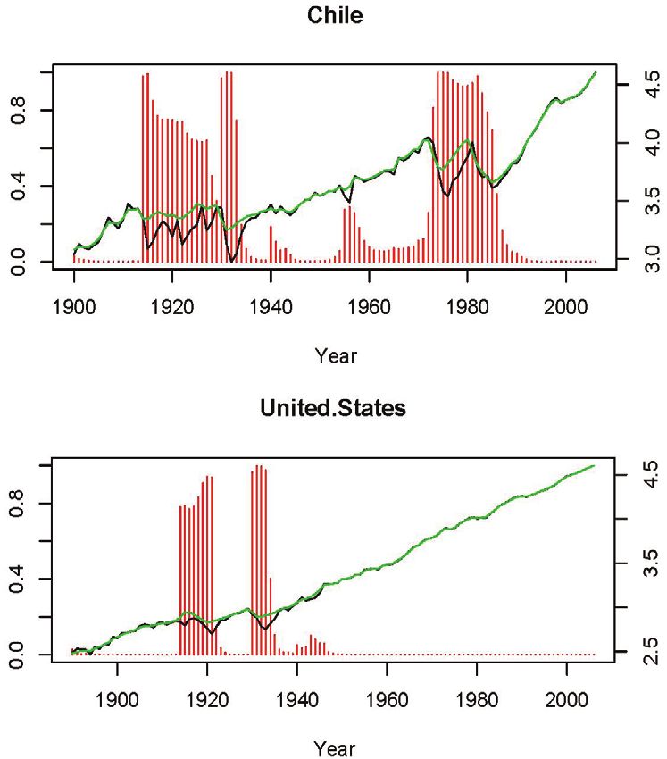
Figure 4. Consumption, Potential Consumption, and Disasters in France, Korea, Chile,
and the United States
Note: In each panel, the dark line is log per capita potential consumption, the lighter line is log per capital poten-
tial consumption, and the bars give our posterior probability estimate that the country was in a disaster in each year.
distribution is particularly important for asset pricing. The median long-run effect
is smaller than the mean long-run effect because the distribution of disaster sizes is
negatively skewed. At first glance, Figure 3 seems to suggest more permanence in
disasters than the typical disaster graph in Figure 2. This pattern arises because the
average short-run effect depicted in Figure 3 averages over many disasters of vary-
ing lengths and is, therefore, muted relative to the individual disasters, which reach
their troughs at different points in time.17
Figure 4 provides more detail about how our model interprets the evolution of
consumption for France, Korea, Chile, and the United States.18 The two lines in each
panel plot consumption and our estimate of potential consumption. The bars give
our posterior probability estimate that a country was in a disaster in each year. For
France, the model picks up World War I and World War II as disasters. The model
views World War II as largely a transitory event for French consumption. The per-
manent effect of World War II on French consumption is estimated to be only about
7 percent. The French experience in World War II is typical for many European
countries. For South Korea, our model interprets the entire period from 1940 to 1960
17
For example, a short disaster may reach its trough after two years, while a long disaster may reach its trough
after ten years. The average drop in consumption at a given point in time (relative to the start of the disaster) is an
average over some disaster paths for which consumption is already recovering after having reached its trough at an
earlier point, and other disaster paths for which consumption is still falling toward a later trough. The trough in aver-
age consumption is, therefore, far less severe than the average of the troughs across different disasters. In contrast,
the long-run average level of consumption is equal to the average of the long-run levels of consumption across the
different disaster paths. It is the fact that the trough in average consumption is so much less than the average of the
troughs that makes the average disaster path look more permanent than in the case of the prototype disaster.
18
More detailed figures for all the countries in our study are reported in online Appendix C.50 American Economic Journal: Macroeconomics July 2013
as a single long disaster that spans World War II and the Korean War. In contrast
to the experience of many European countries, our estimates suggest that the crisis
in the 1940s and 1950s had a large, permanent effect on South Korean consump-
tion (48 percent). This pattern is typical of the experience of Asian countries in our
sample during World War II.
While the bulk of the disasters we identify are associated with world disasters, we
also identify a number of idiosyncratic disaster events. Some of these idiosyncratic
disasters are associated with financial or debt crises. For example, we identify a
disaster in South Korea at the time of the Asian Financial Crisis and in Argentina at
the time of their 2002 sovereign default.19 Other idiosyncratic disasters are associ-
ated with regional wars, coups, or revolutions. These include Chile’s experience
during the 1970s.
The last panel in Figure 4 plots results for the United States. Relative to most
other countries in our sample, the United States was a tranquil place during our
sample period. The model identifies two disaster episodes for the United States. The
first disaster begins in 1914 and lasts until 1922, encompassing both World War I
and the Great Influenza Epidemic of 1918–1920. The Great Depression is identi-
fied as a second disaster for US consumption. The Great Depression is the larger of
the two disasters with a 26 percent short-run drop in consumption and a 14 percent
long-run drop.
One could also ask whether the relative tranquility of the US experience since
the Great Depression provides evidence that the United States is fundamentally dif-
ferent from other countries in our sample. However, the posterior probability for a
randomly selected country experiencing no disasters over a 72-year stretch is 0.12
according to our model. The posterior probability of at least one out of 24 countries
experiencing no disaster over a 73-year stretch is 0.60. Therefore, the tranquility
of the US experience (which is not randomly selected) does not provide evidence
against our model.
Figure 5 plots our estimates of the probability that a “world disaster” began
in each year.20 Our model clearly identifies World War I, the Great Depression,
and World War II as world disasters. Our estimate of pW, the probability that a
world disaster begins, is 3.7 percent per year. Countries are estimated to have
a 62.3 percent probability of entering disasters conditional on a world disaster,
but a much lower (0.6 percent per year) probability of entering a disaster “on
their own.” The overall probability that a country enters a disaster is 2.8 percent
per year.21
Our Bayesian estimation procedure does not deliver a definitive judgment on
whether a disaster occurred at certain times and places, but rather provides a posterior
19
Countries such as Indonesia and Thailand likely also experienced disasters during the Asian Financial Crisis
but are not in the dataset.
20
This is the posterior mean of I W, tfor each year. In other words, with the hindsight of all the data up until 2006,
what is our estimate of whether a world disaster began in say 1940?
21
The overall probability that a country will enter a disaster is pW pCbW + (1 − pW )pC bI. Since the three
parameters involved are not independent, we cannot simply multiply together the posterior mean estimates we
have for them to get a posterior mean of the overall probability of entering a disaster. Instead, we use the joint
posterior distribution of these three parameters to calculate a posterior mean estimate of the overall probability
that a country enters a disaster.Vol. 5 No. 3 Nakamura et al.: Crises and Recoveries 51
1
0.9
0.8
0.7
0.6
0.5
0.4
0.3
0.2
0.1
0
1890 1900 1910 1920 1930 1940 1950 1960 1970 1980 1990 2000
Figure 5. World Disaster Probability
Note: The figure plots the posterior mean of IW, t , i.e., the probability that the world entered a
disaster in each year evaluated using data up to 2006.
probability of whether a disaster occurred. For expositional purposes, however, it is
useful to define “disaster episodes” as periods when the posterior probability of a
disaster is estimated to be particularly high. We define a disaster episode as a set of
consecutive years for a particular country such that: the probability of a disaster in
each of these years is larger than 10 percent, and the sum of the probability of disas-
ter for each year over the whole set of years is larger than one.22 In a few cases, our
model is not able to distinguish between two or more episodes of economic turmoil
that occur in the same country over a short span of time and, therefore, lumps these
events into one long disaster episode.23
Using this definition, we identify 53 disaster episodes. Summary statistics for the
main disaster episodes are reported in Table 2, including the short-run and long-run
effects of the disaster. In all cases, these statistics measure the negative effect of the
disaster on the level of consumption relative to the counterfactual scenario where
the country instead experienced normal trend growth. On average, the maximum
drop in consumption due to the disasters is 29 percent, while the permanent effect
of disasters on consumption is, on average, 14 percent, consistent with our estimates
of the permanent and transitory components of disaster shocks.
22
More formally: A disaster episode is a set of consecutive years for a particular country, T i , such that for all
t ∈ Ti P(Ii, t = 1) > 0.1 and ∑
t∈Tt P(Ii, t = 1) > 1. The idea behind this definition is that there is a substantial
posterior probability of a disaster for a particular set of consecutive years. We stress that the concept of a disaster
episode is purely a descriptive device and does not influence our analysis of asset pricing. One could consider broader
or narrower definitions (lower or higher cutoffs) of disaster episodes. In our experience, there are few borderline cases.
23
Examples include World War II and the Korean war for South Korea, and World War I and the Great
Depression for Chile.52 American Economic Journal: Macroeconomics July 2013
Table 2—Disaster Episodes
Country Start date End date Max drop Perm. drop Perm./Max
Argentina 1890 1908 −0.23 0.02 −0.07
Argentina 1914 1917 −0.13 −0.05 0.37
Argentina 1930 1933 −0.16 −0.10 0.65
Argentina 2000 2004 −0.10 −0.01 0.07
Australia 1914 1923 −0.29 −0.14 0.48
Australia 1930 1934 −0.24 −0.16 0.65
Australia 1939 1956 −0.31 −0.09 0.27
Belgium 1913 1920 −0.40 0.05 −0.12
Belgium 1939 1950 −0.52 −0.14 0.26
Brazil 1930 1932 −0.12 −0.05 0.46
Brazil 1940 1942 −0.07 0.00 0.01
Canada 1914 1926 −0.37 −0.20 0.55
Canada 1930 1933 −0.29 −0.28 0.94
Chile 1914 1934 −0.53 −0.36 0.69
Chile 1955 1958 −0.07 −0.02 0.34
Chile 1972 1987 −0.58 −0.56 0.95
Denmark 1914 1926 −0.16 −0.08 0.54
Denmark 1940 1950 −0.28 −0.11 0.40
Finland 1890 1893 −0.08 −0.01 0.18
Finland 1914 1921 −0.42 −0.22 0.52
Finland 1930 1934 −0.23 −0.11 0.49
Finland 1940 1945 −0.29 −0.14 0.48
France 1914 1921 −0.22 0.08 −0.36
France 1940 1945 −0.56 −0.07 0.12
Germany 1914 1932 −0.45 −0.22 0.48
Germany 1940 1950 −0.48 −0.35 0.71
Italy 1940 1949 −0.33 −0.15 0.45
Japan 1914 1918 −0.04 0.12 −2.73
Japan 1940 1952 −0.61 −0.41 0.67
South Korea 1940 1960 −0.58 −0.48 0.83
South Korea 1997 2004 −0.23 −0.18 0.81
Mexico 1914 1918 −0.16 0.27 −1.66
Mexico 1930 1935 −0.24 −0.06 0.23
Netherlands 1914 1919 −0.45 −0.07 0.15
Netherlands 1940 1952 −0.55 −0.10 0.18
Norway 1914 1924 −0.13 −0.04 0.33
Norway 1940 1944 −0.08 −0.07 0.84
Peru 1930 1933 −0.17 −0.08 0.47
Peru 1977 1993 −0.40 −0.37 0.93
Portugal 1914 1921 −0.28 −0.16 0.56
Portugal 1940 1942 −0.09 −0.07 0.74
Spain 1914 1919 −0.10 0.00 0.02
Spain 1930 1961 −0.59 −0.54 0.91
Sweden 1914 1923 −0.21 −0.15 0.72
Sweden 1940 1951 −0.28 −0.14 0.51
Switzerland 1914 1921 −0.14 −0.09 0.62
Switzerland 1940 1950 −0.23 −0.15 0.65
Taiwan 1901 1916 −0.24 −0.09 0.37
Taiwan 1940 1955 −0.65 −0.46 0.71
United Kingdom 1914 1921 −0.20 −0.10 0.50
United Kingdom 1940 1946 −0.20 −0.08 0.39
United States 1914 1922 −0.24 −0.14 0.57
United States 1930 1935 −0.26 −0.14 0.53
Average −0.29 −0.14 0.42
Median −0.24 −0.10 0.48
Notes: A disaster episode is defined as a set of consecutive years for a particular country such that: (1) the probabil-
ity of a disaster in each of these years is larger than 10 percent, (2) the sum of the probability of disaster for each
year over the whole set of years is larger than one. Max drop is the posterior mean of the maximum shortfall in the
level of consumption due to the disaster. Perm drop is the posterior mean of the permanent effect of the disaster on
the level potential consumption. Perm./Max is the ratio of Perm. drop to Max drop.You can also read