A data-model approach to interpreting speleothem oxygen isotope records from monsoon regions
←
→
Page content transcription
If your browser does not render page correctly, please read the page content below
Clim. Past, 17, 1119–1138, 2021
https://doi.org/10.5194/cp-17-1119-2021
© Author(s) 2021. This work is distributed under
the Creative Commons Attribution 4.0 License.

A data–model approach to interpreting speleothem oxygen
isotope records from monsoon regions
Sarah E. Parker1 , Sandy P. Harrison1 , Laia Comas-Bru1 , Nikita Kaushal2 , Allegra N. LeGrande3 , and
Martin Werner4
1 School of Archaeology, Geography and Environmental Science, University of Reading, Reading, UK
2 Asian School of the Environment, Nanyang Technological University, Singapore, Singapore
3 NASA Goddard Institute for Space Studies and Center for Climate Systems Research, Columbia University, New York, USA
4 Alfred Wegener Institute, Helmholtz Centre for Polar and Marine Research, Bremerhaven, Germany

Correspondence: Sarah E. Parker (s.parker@pgr.reading.ac.uk)

Received: 13 June 2020 – Discussion started: 13 July 2020
Revised: 15 March 2021 – Accepted: 25 March 2021 – Published: 4 June 2021

Abstract. Reconstruction of past changes in monsoon cli-         Australian region. Redundancy analysis shows that 37 % of
mate from speleothem oxygen isotope (δ 18 O) records is          Holocene variability can be accounted for by latitude and
complex because δ 18 O signals can be influenced by mul-         longitude, supporting the differentiation of records into in-
tiple factors including changes in precipitation, precipita-     dividual monsoon regions. Regression analysis of simulated
tion recycling over land, temperature at the moisture source,    precipitation δ 18 O and climate variables show significant re-
and changes in the moisture source region and transport          lationships between global Holocene monsoon δ 18 O trends
pathway. Here, we analyse > 150 speleothem records of            and changes in precipitation, atmospheric circulation and (to
the Speleothem Isotopes Synthesis and AnaLysis (SISAL)           a lesser extent) source area temperature, whereas precipita-
database to produce composite regional trends in δ 18 O in       tion recycling is non-significant. However, there are differ-
monsoon regions; compositing minimises the influence of          ences in regional-scale mechanisms: there are clear relation-
site-specific karst and cave processes that can influence in-    ships between changes in precipitation and δ 18 O for India,
dividual site records. We compare speleothem δ 18 O observa-     southwestern South America and the Indonesian–Australian
tions with isotope-enabled climate model simulations to in-      regions but not for the East Asian monsoon. Changes in at-
vestigate the specific climatic factors causing these regional   mospheric circulation contribute to δ 18 O trends in the East
trends. We focus on differences in δ 18 O signals between        Asian, Indian and Indonesian–Australian monsoons, and a
the mid-Holocene, the peak of the Last Interglacial (Marine      weak source area temperature effect is observed over south-
Isotope Stage 5e) and the Last Glacial Maximum as well           ern and central America and Asia. Precipitation recycling
as on δ 18 O evolution through the Holocene. Differences in      is influential in southwestern South America and southern
speleothem δ 18 O between the mid-Holocene and the Last In-      Africa. Overall, our analyses show that it is possible to dif-
terglacial in the East Asian and Indian monsoons are small,      ferentiate the impacts of specific climatic mechanisms influ-
despite the larger summer insolation values during the Last      encing precipitation δ 18 O and use this analysis to interpret
Interglacial. Last Glacial Maximum δ 18 O values are signif-     changes in speleothem δ 18 O.
icantly less negative than interglacial values. Comparison
with simulated glacial–interglacial δ 18 O shows that changes
are principally driven by global shifts in temperature and
regional precipitation. Holocene speleothem δ 18 O records       1   Introduction
show distinct and coherent regional trends. Trends are sim-
ilar to summer insolation in India, China and southwestern       The oxygen isotopic (δ 18 O; the 18 O/16 O ratio relative to a
South America, but they are different in the Indonesian–         standard, in per mille, ‰) composition of speleothems is
                                                                 widely used to infer past regional climates (Bar-Matthews et

Published by Copernicus Publications on behalf of the European Geosciences Union.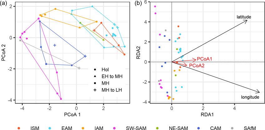
1120                                                    S. E. Parker et al.: Interpreting speleothem records of monsoon changes

al., 1997; McDermott, 2004; Wang et al., 2008). Speleothem              cipitation (Cheng et al., 2013; Fleitmann et al., 2003) or a
oxygen isotope (δ 18 Ospel ) signals are inherited from δ 18 O in       change in the ratio of more negative δ 18 O summer precip-
precipitation (δ 18 Oprecip ) above the cave, which in turn is de-      itation to less negative δ 18 O winter precipitation (Dong et
termined by the initial δ 18 O of water vapour as it evaporates         al., 2010; Wang et al., 2001). However, the multiplicity of
at the oceanic moisture source region, the degree of rainout            processes that influence δ 18 O before its incorporation in the
and evaporation from source to cave site, and air tempera-              speleothem makes it difficult to attribute the climatic causes
ture changes encountered throughout the moisture transport              of changes in individual speleothem records unambiguously.
pathway (Fairchild and Baker, 2012; Lachniet, 2009). Under-             In the East Asian monsoon, for example, speleothem δ 18 O
standing the effects and contribution of each of these climate          records have been interpreted as a summer monsoon sig-
processes to δ 18 Oprecip (and therefore δ 18 Ospel ) is essential to   nal, manifested as a change in the amount of water vapour
inferring palaeoclimate from speleothem δ 18 O records.                 removed along the moisture trajectory (Yuan et al., 2004),
    Initial δ 18 O is determined by oceanic δ 18 O at the evap-         and/or as a change in the contribution of summer precip-
orative moisture source region (Craig and Gordon, 1965),                itation to annual totals (Cheng et al., 2006, 2009, 2016;
which varies spatially (LeGrande and Schmidt, 2006) and                 Wang et al., 2001) based on the relationship between modern
through time (e.g. Waelbroeck et al., 2002). During evapora-            δ 18 Oprecip and climate. Other interpretations of Chinese mon-
tion from the moisture source, 16 O is preferentially incorpo-          soon δ 18 Ospel have included rainfall source changes (Tan,
rated into the vapour, whilst subsequent fractionation during           2009, 2011, 2014) or local rainfall changes (Tan et al., 2015).
atmospheric transport occurs by Rayleigh distillation; as air           Maher (2008) interpreted δ 18 Ospel as reflecting changes in
masses cool and moisture condenses, heavier 18 O is enriched            moisture source area, based on differences between δ 18 Ospel
in the liquid phase and removed by precipitation. With pro-             and loess/palaeosol records of rainfall and the strong corre-
gressive rainout along a moisture pathway, precipitation be-            lation between East Asian and Indian monsoon speleothems.
comes gradually more depleted (Dansgaard, 1964). Within                 Maher and Thompson (2012) used a mass balance approach
this framework, δ 18 Oprecip is controlled by two variables:            to show that the changes in precipitation (either local or up-
temperature and the amount of precipitation along a mois-               stream) or rainfall seasonality required to reproduce δ 18 Ospel
ture pathway. The temperature effect stems from the cooling             trends would be unreasonably large. Thus, they argued that
required for progressive rainout during Rayleigh distillation           changes in moisture source were required to explain shifts in
(Dansgaard, 1964; Rozanski et al., 1993). The temperature-              δ 18 O both on glacial–interglacial timescales and during in-
δ 18 O impact is dominant at mid to high latitudes, whilst ob-          terglacials. Overall, there are several plausible climate mech-
servations suggest that changes in upstream and local pre-              anisms that could contribute to δ 18 Ospel on multi-millennial
cipitation dominate changes in the δ 18 Oprecip signal at trop-         timescales. East Asian monsoon speleothem records are of-
ical latitudes. The negative relationship between local pre-            ten interpreted as a combination of several of these processes
cipitation and δ 18 Oprecip , often referred to as the “amount ef-      (Cheng et al., 2016; Dykoski et al., 2005) which generally
fect” (Bailey et al., 2018; Dansgaard, 1964), results from the          represent monsoon intensity (Cheng et al., 2019). There are
re-evaporation and diffusive exchange between precipitation             also multiple interpretations of the causes of δ 18 Ospel vari-
and water vapour during deep convective precipitation (Risi             ability in other monsoon regions. In the Indian monsoon re-
et al., 2008). However, Rayleigh distillation is complicated            gion, speleothem δ 18 O records are interpreted primarily as
by changes in atmospheric circulation and moisture recy-                an amount effect signal (Berkelhammer et al., 2010; Fleit-
cling. Changes in the area from which the moisture is sourced           mann et al., 2004), supported by modern δ 18 Oprecip and cli-
will modify δ 18 Oprecip because the initial δ 18 O values differ       mate observations (e.g. Battacharya et al., 2003). However,
between sources (Cole et al., 1999; Friedman et al., 2002),             other studies have suggested that δ 18 Oprecip changes in this
whilst changes in the moisture transport pathway and/or dis-            region are driven primarily by large-scale changes in mon-
tance between the source and cave site can result in differing          soon circulation; hence, Indian monsoon δ 18 Ospel should
degrees of fractionation associated with condensation and               be interpreted as a moisture source and/or trajectory sig-
evaporation (Aggarwal et al., 2012; Bailey et al., 2018). The           nal (Breitenbach et al., 2010; Sinha et al., 2015). In the
isotopic composition of atmospheric water vapour may also               Indonesian–Australian monsoon region, δ 18 Ospel variability
be modified by precipitation recycling over land, as evapo-             has been interpreted as a precipitation amount signal (Car-
transpiration returns moisture from precipitation back to the           olin et al., 2016; Krause et al., 2019) or a precipitation sea-
atmosphere, thereby minimising the δ 18 Oprecip /distance gra-          sonality signal (Ayliffe et al., 2013; Griffiths et al., 2009),
dient along an advection path that occurs with Rayleigh dis-            based on modern δ 18 Oprecip and climate observations (Cobb
tillation (Gat, 1996; Salati et al., 1979).                             et al., 2007; Moerman et al., 2013), and/or as a moisture
    Speleothem δ 18 O records from monsoon regions show                 source and/or trajectory signal (Griffiths et al., 2009; Wurtzel
multi-millennial variability that has been interpreted as doc-          et al., 2018). South American speleothem records have been
umenting the waxing and waning of the monsoons in re-                   interpreted as records of monsoon intensity, due to changes in
sponse to changes in summer insolation, often interpreted               the amount of precipitation over the region (Cruz et al., 2005;
predominantly as a change in the absolute amount of pre-                Wang et al., 2006; Cheng et al., 2013), changes in the degree

Clim. Past, 17, 1119–1138, 2021                                                            https://doi.org/10.5194/cp-17-1119-2021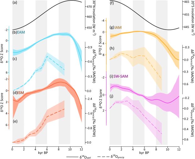
S. E. Parker et al.: Interpreting speleothem records of monsoon changes                                                         1121

of upstream precipitation and evapotranspiration (Cheng et           trends observed in speleothem records across specific mon-
al., 2013), or changes in the ratio of precipitation sourced         soon regions, using multiple regression analysis.
from the low-level jet versus the Atlantic (Cruz et al., 2006;
Wang et al., 2006).
                                                                     2     Methods
   These interpretations generally rely on modern δ 18 Oprecip
and climate observations, which may not have remained con-
                                                                     2.1    Speleothem oxygen isotope data
stant through time. The sources of δ 18 O variability can also
be explored using isotope-enabled climate models (e.g. Hu            Speleothem δ 18 O records were obtained from the SISAL
et al., 2019), which incorporate known isotope effects and,          (Speleothem Isotopes Synthesis and AnaLysis) database (At-
therefore, provide plausible explanations for δ 18 Ospel trends.     sawawaranunt et al., 2018; Comas-Bru et al., 2020a, b).
Modelling studies suggest that changes in East Asian mon-            Records were selected based on the following criteria:
soon δ 18 Oprecip , during Heinrich events (Lewis et al., 2010;
Pausata et al., 2010) and on an orbital timescale (Battisti et           – they are located in monsoon regions, between 35◦ S and
al., 2014; LeGrande and Schmidt, 2009), do not reflect lo-                 40◦ N;
cal rainfall variability but instead reflect changes in the δ 18 O
of vapour delivered to the region. Variability in the δ 18 O             – the mineralogy is known and does not vary (i.e. be-
of vapour delivered to East Asia on orbital timescales has                 tween calcite and aragonite) through time, because oxy-
been diagnosed as being due to changes in precipitation up-                gen isotope fractionation during speleothem precipita-
stream of the region (Battisti et al., 2014), changes in mois-             tion is different for calcite and aragonite;
ture source location (Hu et al., 2019; Tabor et al., 2018)
                                                                         – for the analysis of mid-Holocene (MH), Last Glacial
or changes in the strength of monsoon winds (LeGrande
                                                                           Maximum (LGM) and Marine Isotope Stage 5e dur-
and Schmidt, 2009; Liu et al., 2014). δ 18 Oprecip variabil-
                                                                           ing the Last Interglacial (LIG) δ 18 O signals, the records
ity in the East Asian monsoon during Heinrich events has
                                                                           contain samples within at least one of these time pe-
also been attributed to non-local isotope fractionation (Lewis
                                                                           riods, defined as 6000 ± 500 years BP for the MH,
et al., 2010; Pausata et al., 2011). Modelling results sug-
                                                                           21 000 ± 1000 years BP for the LGM and 125 000 ±
gest that changes in precipitation amount are the predomi-
                                                                           1000 years BP for the LIG, where BP (before present)
nant source of δ 18 O variability in the Indian monsoon dur-
                                                                           is 1950 CE;
ing the Holocene (LeGrande and Schmidt, 2009) and in the
glacial (Lewis et al., 2010) as well as in the South American
                                                                         – for the PCoA, the records have a temporal coverage of
and Indonesian–Australian regions during Heinrich events
                                                                           at least 4000 years in the Holocene;
(Lewis et al., 2010) and the Last Interglacial (Sjolte and Hoff-
man, 2014).                                                              – for Holocene trend analyses, speleothems have a record
   In this study, we combine speleothem δ 18 O records of                  of the period from 7000 to 3000 years BP;
the Speleothem Isotopes Synthesis and AnaLysis (SISAL)
database with isotope-enabled palaeoclimate simulations                  – they are the most recent update of the record from a site
from two climate models to investigate the plausible mecha-                available in version 2 of the SISAL database.
nisms driving changes in δ 18 O in monsoon regions through
the Holocene (last 11 700 years) and between the mid-                This resulted in the selection of 125 records from 44 sites for
Holocene, the peak of the Last Interglacial and the Last             the PCoA analysis, 64 records from 38 sites for the analy-
Glacial Maximum. We compare δ 18 Ospel signals across ge-            sis of MH, LGM and LIG signals, and 79 records from 40
ographically separated cave sites to extract a regional signal,      sites for the Holocene trend analysis (Fig. 1). Although the
thereby minimising the influence of karst and in-cave pro-           SISALv2 database contains multiple age models for some
cesses, such as the mixing of groundwaters from different            sites, we use the published age models given by the original
precipitation events or changes in cave ventilation, that can        authors for all records.
be important for the δ 18 Ospel of individual records. We use
principal coordinate analysis (PCoA) to identify regions with        2.2    Climate model simulations
geographically coherent δ 18 Ospel records and then examine
how these regions behave on glacial–interglacial timescales          There are relatively few palaeoclimate simulations made
and through the Holocene. We use isotope-enabled model               with models that incorporate oxygen isotope tracers, and the
simulations to investigate the potential causes of δ 18 Ospel        available simulations do not necessarily focus on the same
variability in regions where the models reproduce the large-         periods or use the same modelling protocols. Here, we use
scale δ 18 O changes shown by observations. We exploit the           simulations of opportunity from two isotope-enabled climate
fact that models produce internally physically consistent            models: ECHAM5 (version 5 of the European Centre for
changes to explore potential and plausible causes of the             medium-range weather forecasting model in HAMburg) and
                                                                     GISS ModelE-R (Goddard Institute for Space Studies Model

https://doi.org/10.5194/cp-17-1119-2021                                                          Clim. Past, 17, 1119–1138, 2021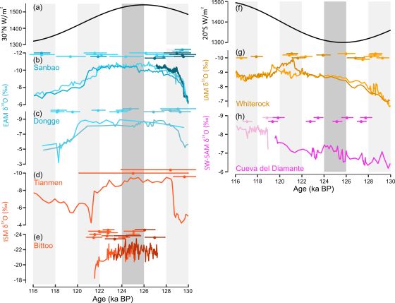
1122                                                   S. E. Parker et al.: Interpreting speleothem records of monsoon changes

Figure 1. Spatial distribution of speleothem records used is this study. Colours indicate the sites used in principal coordinates analysis
(PCoA) and redundancy analysis (RDA) to separate monsoon regions, and sites not used in PCoA and RDA but used in subsequent analyses.
The individual regional monsoons are shown by boxes: CAM denotes the Central American monsoon (latitude from 10 to 33◦ , longitude
from −115 to −58◦ ), SW-SAM denotes the southwestern South American monsoon (latitude from −10 to 0◦ , longitude from −80 to −64◦ ;
latitude from −30 to −10◦ , longitude −68 to −40◦ ), NE-SAM denotes the northeastern South American monsoon (latitude from −10 to 0◦ ,
longitude: −60 to −30◦ ), SAfM denotes the southern African monsoon (latitude from −30 to −17◦ , longitude from 10 to 40◦ ), ISM denotes
the Indian summer monsoon (latitude from 11 to 32◦ , longitude from 50 to 95◦ ), EAM denotes the East Asian monsoon (latitude from 20
to 39◦ , longitude from 100 to 125◦ ) and IAM denotes the Indonesian–Australian monsoon (latitude from −24 to 5◦ , longitude from 95 to
135◦ ). Source region limits used in the multiple linear regression analysis are also shown. The background carbonate lithology is from the
WOrld Karst Aquifer Mapping (WOKAM) project (Goldschneider et al., 2020).

version E-R). The ECHAM5 simulations provide an oppor-                  MH and LGM simulations were run at T106 horizontal grid
tunity to examine large-scale changes between glacial and in-           resolution, approximately 1.1◦ × 1.1◦ at the Equator. Com-
terglacial states, using simulations of the MH, LGM and LIG.            parison of the MH and LGM simulations with speleothem
The GISS ModelE-R ocean–atmosphere coupled general cir-                 data globally (Figs. S1 and S2 in the Supplement; Comas-Bru
culation model was used to investigate the evolution of δ 18 O          et al., 2019) show that the ECHAM model reproduces the
evolution during the Holocene, using eight time slice (9, 6,            broadscale spatial gradients and the sign of isotopic changes
5, 4, 3, 2, 1 and 0 ka) experiments. Although simulations of            at the majority of cave sites (MH: 72 %; LGM: 76 %). How-
the MH 6 ka time slice are available with both models, there            ever, the changes compared with present are generally more
are differences in the protocol used for the two experiments            muted in the simulations than shown by the speleothem
which preclude direct comparison of the simulations.                    records.
   The ECHAM5-wiso MH experiment (Wackerbarth et                           The LIG experiment (Gierz et al., 2017b, a) was run us-
al., 2012; Werner, 2019) was forced by orbital parameters               ing the ECHAM5/MPI-OM Earth system model, with sta-
(based on Berger and Loutre, 1991) and greenhouse gas                   ble water isotope diagnostics included in the ECHAM5 at-
(GHG) concentrations (CO2 = 280 ppm, CH4 = 650 ppb,                     mosphere model (Werner et al., 2011), the dynamic vege-
N2 O = 270 ppb) appropriate to 6 ka. Changes in sea surface             tation model JSBACH (Haese et al., 2012) and the MPI-
temperature (SST) and sea ice were derived from a tran-                 OM ocean–sea-ice module (Xu et al., 2012). This simula-
sient Holocene simulation (Varma et al., 2012). The con-                tion was run at a T31L19 horizontal grid resolution, approx-
trol simulation for the MH experiment was an ECHAM-                     imately 3.75◦ × 3.75◦ . The LIG simulation was forced by
wiso simulation of the period from 1956 to 1999 (Lange-                 orbital parameters derived from Berger and Loutre (1991)
broek et al., 2011), using observed SSTs and sea ice                    and GHG concentrations (CO2 = 276 ppm, CH4 = 640 ppb,
cover. This control experiment was forced by SSTs and sea               N2 O = 263 ppb) appropriate to 125 ka, but it was assumed
ice only, with atmospheric circulation free to evolve. The              that the ice sheet configuration and land–sea geography re-
ECHAM5-wiso LGM experiment (Werner, 2019; Werner                        main unchanged from modern; therefore no change was
et al., 2018) was forced by orbital parameters (Berger                  made to the isotopic composition of sea water. The LIG sim-
and Loutre, 1991), GHG concentrations (CO2 = 185 ppm,                   ulation is compared to a pre-industrial (PI) control with ap-
CH4 = 350 ppb, N2 O = 200 ppb), land–sea distribution and               propriate insolation, GHG and ice sheet forcing for 1850 CE.
ice sheet height and extent appropriate to 21 ka; SST and               The sign of simulated isotopic changes in the LIG is in good
sea ice cover were prescribed from the GLAMAP dataset                   agreement with ice core records from Antarctica and Green-
(Schäfer-Neth and Paul, 2003). Sea surface water and sea ice            land and speleothem records from Europe, the Middle East
δ 18 O were uniformly enriched by 1 ‰ at the start of the ex-           and China (Gierz et al., 2017b), although, as with the MH
periment. The control simulation for the LGM experiment                 and LGM, the observed changes tend to be larger than the
used present-day conditions, including orbital parameters               simulated changes (Fig. S3).
and GHG concentrations set to modern values, and SSTs and                  There are GISS ModelE-R (LeGrande and Schmidt, 2009)
sea ice cover from the last 20 years (1979–1999). Both the              simulations for eight time slices during the Holocene (9, 6, 5,

Clim. Past, 17, 1119–1138, 2021                                                             https://doi.org/10.5194/cp-17-1119-2021
S. E. Parker et al.: Interpreting speleothem records of monsoon changes                                                    1123

4, 3, 2, 1 and 0 ka). The 0 ka experiment is considered as the    2.4   Glacial–interglacial changes in δ 18 O
pre-industrial control (ca. 1880 CE). Orbital parameters were
                                                                  We examined shifts in δ 18 Ospel observations and in annual
based on Berger and Loutre (1991), and GHG concentrations
                                                                  precipitation-weighted mean δ 18 Oprecip from ECHAM-wiso
were adjusted based on ice core reconstructions (Brook et
                                                                  in regions influenced by the monsoon, between the MH,
al., 2000; Indermühle et al., 1999; Sowers, 2003) for each
                                                                  LGM and LIG. Values are given as anomalies with respect
time slice. A remnant Laurentide ice sheet was included in
                                                                  to the present day for speleothems or the control simulation
the 9 ka simulation, following Licciardi et al. (1998), and the
                                                                  experiment for model outputs. Comas-Bru et al. (2019) have
corresponding adjustment was made to mean ocean salin-
                                                                  shown that differences in speleothem δ 18 O data between the
ity and ocean water δ 18 O to account for this (Carlson et
                                                                  20th century and the pre-industrial period (i.e. 1850±15 CE)
al., 2008). The ice sheet in all the other experiments was
                                                                  are within the temporal and measurement uncertainties of
specified to be the same as modern; therefore, no adjustment
                                                                  the data; thus, the use of different reference periods (i.e. PI
was necessary. The simulations were run using the M20 ver-
                                                                  for the ECHAM LIG experiment, 20th century for ECHAM
sion of GISS ModelE-R, which has a horizontal resolution of
                                                                  MH, LGM experiments) should have little effect on our anal-
4◦ × 5◦ . Each experiment was run for 500 years, and we use
                                                                  yses. We used mean site δ 18 Ospel values for each period for
the last 100 simulated years for the analyses. Comparison
                                                                  the regions identified in the PCoA analysis. Where there are
of the simulated trends in δ 18 O show good agreement with
                                                                  multiple speleothem δ 18 O records for a site in a time pe-
Greenland ice core records, marine records from the tropi-
                                                                  riod, they were averaged to calculate mean δ 18 Ospel . Three
cal Pacific and Chinese speleothem records (LeGrande and
                                                                  sites above 3500 m were excluded from the calculation of
Schmidt, 2009). However, as is the case with the ECHAM
                                                                  the means because high-elevation sites have more negative
simulations, the model tends to produce changes that are
                                                                  δ 18 O values than their low-elevation counterparts, and their
less extreme than those shown by the observations (Figs. S4,
                                                                  inclusion would distort the regional estimates.
S5, S6).
                                                                     There are relatively few speleothems covering both the
                                                                  present day and the period of interest (i.e. MH, LGM or LIG),
2.3   Principal coordinate analysis and redundancy                precluding the calculation of δ 18 Ospel anomalies from the
      analysis                                                    speleothem data. Therefore, we calculated anomalies with re-
                                                                  spect to the modern period (1960–2017 CE) using the Online
We used PCoA to identify regionally coherent patterns in
                                                                  Isotopes in Precipitation Calculator (OIPC: Bowen, 2018;
the speleothem δ 18 O records for the Holocene. PCoA is a
                                                                  Bowen and Revenaugh, 2003), a global gridded dataset of
multivariate ordination technique that uses a distance ma-
                                                                  interpolated mean annual precipitation-weighted δ 18 Oprecip
trix to represent inter-object (dis)similarity in reduced space
                                                                  data, as reference. This dataset combines data from 348
(Gower, 1966; Legendre and Legendre, 1998). Speleothem
                                                                  stations from the Global Network of Isotopes in Precipita-
records from individual sites are often discontinuous; miss-
                                                                  tion (IAEA/WMO, 2018), covering part or all of the 1960–
ing data are problematic for many ordination techniques.
                                                                  2014 period, and other records available at the Waterisotopes
PCoA is more robust to missing data than other methods
                                                                  Database (Waterisotopes Database, 2017).
(Kärkkäinen and Saarela, 2015; Rohlf, 1972). We used a cor-
                                                                     OIPC δ 18 Oprecip was converted to its speleothem equiv-
relation matrix of speleothem records as the (dis)similarity
                                                                  alent assuming that (i) precipitation-weighted mean annual
measure. The temporal resolution of speleothem records was
                                                                  δ 18 Oprecip is equivalent to mean annual drip-water δ 18 O
first standardised by calculating a running average mean
                                                                  (Yonge et al., 1985) and that (ii) precipitation of calcite is
with non-overlapping 500-year windows. This procedure
                                                                  consistent with the empirical speleothem-based kinetic frac-
produces a single composite record when there are several
                                                                  tionation factor of Tremaine et al. (2011) and precipitation
records for a given site. PCoA results were displayed as
                                                                  of aragonite follows the fractionation factor from Grossman
a biplot, where sites ordinated close to one another (i.e.
                                                                  and Ku (1986), as formulated by Lachniet (2015):
with similar PCoA scores) show similar Holocene trends,
and sites ordinated far apart have dissimilar trends. We used     δ 18 Ocalcite_SMOW = wδ 18 Oprecip_SMOW
the “broken stick” model (Bennett, 1996) to identify which
PCoA axes were significant. We used redundancy analy-                         16.1 · 1000
                                                                      +                     − 24.6    (T in K),              (1)
sis (RDA: Legendre and Legendre, 1998; Rao, 1964) with                            T
latitude and longitude as predictor variables to identify if
PCoA (dis)similarities were related to geographical loca-
tion, and principal components analysis (PCA) to identify the     δ 18 Oaragonite_SMOW = wδ 18 Oprecip_SMOW

main patterns of variation. As these explanatory variables are               18.34 · 1000
not dimensionally homogeneous, they were centred on their             +                     − 31.954     (T in K),           (2)
                                                                                   T
means and standardised to allow direct comparison of the
gradients. PCoA and RDA analyses were carried out using           where δ 18 Ocalcite_SMOW and δ 18 Oaragonite_SMOW are the re-
the “vegan” package in R (Oksanen et al., 2019).                  spective speleothem isotopic composition for calcite and

https://doi.org/10.5194/cp-17-1119-2021                                                      Clim. Past, 17, 1119–1138, 2021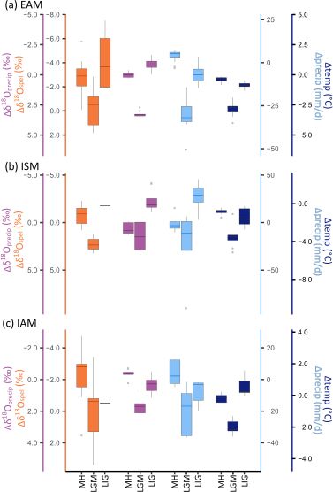
1124                                               S. E. Parker et al.: Interpreting speleothem records of monsoon changes

aragonite speleothems with reference to the VSMOW (Vi-                  mean and variance:
enna Standard Mean Ocean Water) standard (in per mille),                                                        .
wδ 18 Oprecip is the OIPC precipitation-weighted annual mean            z scorei = δ 18 Oi − δ 18 O(base period)    sδ 18 O(base period) , (4)
isotopic composition of precipitation with respect to the VS-
MOW standard and T is the mean annual cave temperature                  where δ 18 O is the mean, and sδ 18 O is the standard devi-
(in kelvin). We used the long-term (1960–2016) mean an-                 ation of δ 18 O for a common base period. A base period
nual surface air temperature from the CRU-TS4.01 database               of 7000 to 3000 years BP was chosen to maximise the
(Harris and Jones, 2017; Harris et al., 2020) at each site as a         number of records included in each composite.
surrogate for mean annual cave air temperature. The resolu-
tion of the gridded data means that wδ 18 Oprecip_SMOW and T       2. The standardised data for a site were resampled by ap-
may be the same for nearby sites.                                     plying a 100-year non-overlapping running mean with
   We use the VSMOW to VPDB (Vienna Pee Dee Belem-                    the first bin centred at 50 years BP, in order to create
nite) conversion from Coplen et al. (1983), which is indepen-         a single site time series while ensuring that highly re-
dent of speleothem mineralogy:                                        solved records do not dominate the regional composite.

δ 18 OPDB = 0.97001 · δ 18 OSMOW − 29.29,                  (3)     3. Each regional composite was constructed using locally
                                                                      weighted regression (Cleveland and Devlin, 1988) with
where δ 18 OPDB is relative to the VPDB standard, and                 a window width of 3000 years and fixed target points in
δ 18 OSMOW is relative to VSMOW standard.                             time.
   Average uncertainties in the speleothem age–depth models
are ∼ 50 years during the Holocene. This interval is smaller       4. Confidence intervals (5th and 95th percentiles) for each
than the time windows used in this analysis; therefore, the           composite were generated by bootstrap resampling by
age uncertainty is expected to have a negligible impact on the        site over 1000 iterations.
results. We investigated the influence of age uncertainties on
                                                                  There are too few sites to construct regional composites for
the LGM and LIG δ 18 Ospel anomalies by examining the im-
                                                                  the peak of the LIG (Marine Isotope Stage 5e); thus, the
pact of using different window widths (±500, ±700, ±1000,
                                                                  trends in δ 18 Ospel were examined using records from indi-
±2000 years) on the regional mean δ 18 Ospel anomalies.
                                                                  vidual sites covering the period from 130 to 116 ka BP.
   We used anomalies of wδ 18 Oprecip , mean annual sur-
                                                                     We calculated Holocene regional composites from annual
face air temperature (MAT) and mean annual precipitation
                                                                  precipitation-weighted mean δ 18 Oprecip anomalies simulated
(MAP) from the ECHAM5-wiso simulations to investigate
                                                                  by the GISS model. Simulated δ 18 Oprecip trends were calcu-
the changes in δ 18 Ospel between the MH, LGM and LIG as
                                                                  lated using linear distance-weighted mean δ 18 Oprecip values
well as their association with changes in climate. Values were
                                                                  from land grid cells (> 50 % land) within ±4◦ around each
calculated from land grid cells (> 50 % land) ±3◦ around
                                                                  site. This distance was determined by the grid resolution of
each speleothem site. This distance was chosen with refer-
                                                                  the model. Regional composites were then produced using
ence to the coarsest-resolution simulation (LIG, ca. 3.75◦ ×
                                                                  bootstrap resampling in the same way as for the speleothem
3.75◦ ). Gridded values of MAT and MAP were weighted by
                                                                  data. The simulated anomalies are relative to the control run
the proportion of each grid cell that lies within ±3◦ of the
                                                                  rather than the specified base period used for the speleothem-
site, and linear distance-weighted means were calculated for
                                                                  based composites, so absolute values of simulated and ob-
each site and time slice. We only considered regions with
                                                                  served Holocene trends are expected to differ. Preliminary
at least one speleothem record for each of the three time
                                                                  analyses showed that neither the mean values nor trends in
periods, although these were not required to be the same
                                                                  δ 18 Oprecip were substantially different if the sampled area
sites, and where the observed shifts in δ 18 Ospel were in the
                                                                  was reduced to match the sampling used for the ECHAM-
same direction and of a similar magnitude to the simulated
                                                                  based box plot analysis, or was increased to encompass the
wδ 18 Oprecip .
                                                                  larger regions shown in Fig. 1 and used in the multiple re-
                                                                  gression analysis.
2.5    Holocene and Last Interglacial regional trends
Regional speleothem δ 18 O changes through the Holocene           2.6   Multiple regression analysis
were examined by creating composite time series for each
region identified in the PCoA analysis with at least four         We investigate the underlying relationships between re-
Holocene records (> 5000 years long). Regional composites         gional δ 18 Oprecip (and by extension δ 18 Ospel and mon-
were constructed using a four-step procedure, modified from       soon climate through the Holocene using multiple linear
Marlon et al. (2008):                                             regression (MLR). We use annual precipitation-weighted
                                                                  mean δ 18 Oprecip anomalies and climate variables from GISS
 1. The δ 18 O data for individual speleothems were trans-        ModelE-R. Climate variables were chosen to represent the
    formed to z scores, so all records have a standardised        four potential large-scale drivers of regional changes in the

Clim. Past, 17, 1119–1138, 2021                                                         https://doi.org/10.5194/cp-17-1119-2021
S. E. Parker et al.: Interpreting speleothem records of monsoon changes 1125
speleothem δ 18 O records. Specifically, we use changes in Table 1. Results of the principal coordinates analysis (PCoA). Sig-
mean precipitation and precipitation recycling over the mon- nificant axes, as determined by the broken stick method (Bennett,
soon regions, and changes in mean surface air tempera- 1996), are shown in bold.
ture and surface wind direction over the moisture source re-
gions. Whereas the influence of changes in precipitation, re- PCoA1 PCoA2 PCoA3 PCoA4 PCoA5
cycling and temperature are relatively direct measures, the Eigenvalue 269.06 85.22 16.81 10.25 5.55
change in surface wind direction over the moisture source Explained (%) 64.87 20.55 4.054 2.47 1.34
Cumulative (%) 64.87 85.42 89.48 91.95 93.27
region is used as an index of potential changes in the mois-
ture source region and transport pathway. The boundaries of
each monsoon region (Fig. 1) were defined to include all
the speleothem sites used to construct the Holocene δ 18 Ospel tionship between each predictor variable and δ 18 Oprecip when
composites. Moisture source area limits (Fig. 1) were defined the effects of the other variables are held constant.
based on moisture tracking studies (Bin et al., 2013; Breit- All statistical analyses were performed in R (R Core Team,
enbach et al., 2010; D’Abreton and Tyson, 1996; Drumond 2019), and plots were generated using ggplot (Wickham,
et al., 2008, 2010; Durán-Quesada et al., 2010; Kennett et 2016).
al., 2012; Nivet et al., 2018; Wurtzel et al., 2018) and GISS
simulated summer surface winds. All climate variables were
3 Results
extracted for the summer months, defined as May to Septem-
ber (MJJAS) for Northern Hemisphere regions and Novem- 3.1 Principal coordinate analysis and redundancy
ber to March (NDJFM) for Southern Hemisphere regions analysis
(Wang and Ding, 2008) on the basis that these regions are
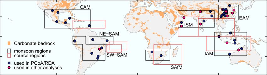
dominated by summer season precipitation (Fig. S7). Only PCoA shows the (dis)similarity of Holocene δ 18 Ospel evo-
grid cells with > 50 % land were used to extract variables lution across individual records and, thus, allows an objec-
over monsoon regions, and only grid cells with < 50 % land tive regionalisation of these records. The first two PCoA
were used to extract variables over moisture source regions. axes are significant, according to the broken stick test, and
The inputs to the MLR for each time interval were calculated account for 65 % and 20 % of δ 18 Ospel variability respec-
as anomalies from the control run. tively (Table 1). The PCoA scores differentiate records ge-
Precipitation recycling was calculated as the ratio of lo- ographically (Fig. 2a): Southern Hemisphere monsoon re-
cally sourced precipitation versus total precipitation. Al- gions such as the southwestern South American monsoon
though the GISS ModelE-R mid-Holocene experiment ex- (SW-SAM) and South African monsoon (SAfM) are charac-
plicitly estimates recycling using vapour source distribution terised by low PCoA1 scores, whereas Northern Hemisphere
tracers (Lewis et al., 2014), this was not done for all the monsoons such as the Indian summer monsoon (ISM) and
Holocene time slice simulations. Therefore, we calculate the East Asian monsoon (EAM) are characterised by higher
a precipitation recycling index (RI), following Brubaker et PCoA1 scores. This indicates that regions can be differen-
al. (1993): tiated based on their temporal evolution as captured by the
first PCoA axis. Most Southern Hemisphere regions also
PR E have lower PCoA2 scores, although this is not consistent
RI = = , (5)
P 2QH + E over time. Speleothem records from the Central American
monsoon (CAM) and the Indonesian–Australian monsoon
where locally sourced (recycled) precipitation (PR ) is esti- (IAM) have PCoA scores that are an intermediate between
mated using total evaporation over a region (E), and total the Northern Hemisphere and Southern Hemisphere regions.
precipitation (P ) is estimated as the sum of total evaporation PCoA clearly separates the South American records into a
and net incoming moisture flux integrated across the bound- northeastern region (NE-SAM), with scores similar to other
aries of the region (QH ). Therefore, RI expresses the change Northern Hemisphere monsoon regions, and a southwest-
in the contribution of local, recycled precipitation indepen- ern region (SW-SAM), with scores similar to other Southern
dently of any overall change in precipitation amount. Hemisphere regions. The RDA supports a geographical con-
We incorporate mean meteorological variables and trol on the (dis)similarity of speleothem δ 18 O records over
δ 18 Oprecip for all Holocene time slices (1 to 9 ka) and all mon- the Holocene (Fig. 2b). RDA1 explains 37 % of the variabil-
soon regions into the MLR model. Thus, the relationships ity and is significantly correlated with both latitude and lon-
constrained by the overall (global) MLR model represent the gitude (Table 2).
combined response across all monsoon regions. We use the
pseudo-R 2 to determine the goodness of fit for the global 3.2 Regional interglacial–glacial differences
MLR model and t values (the regression coefficient divided
by its standard error) to determine the strength of each re- To investigate the causes of shifts in δ 18 O between the MH,
lationship. Partial residual plots were used to show the rela- LGM and LIG, we compare simulated and observed regional
https://doi.org/10.5194/cp-17-1119-2021 Clim. Past, 17, 1119–1138, 20211126 S. E. Parker et al.: Interpreting speleothem records of monsoon changes Figure 2. Results of the principal coordinate analysis (PCoA) and redundancy analysis (RDA). (a) PCoA biplot showing the loadings of each site on the first two axes, which represent 85 % of the total variance. Shapes indicate the Holocene coverage of each site, where sites with a coverage ≥ 8000 years represent most or all of the Holocene (Hol). Sites with a temporal coverage of < 8000 years are coded to show whether they represent the early Holocene to mid-Holocene (EH to MH; record midpoint > 8000 years BP), the mid-Holocene (MH; record midpoint between 8000 and 5000 years BP) or the mid-Holocene to late Holocene (LH to MH; midpoint < 5000 years BP). (b) RDA triplot, where the response variables are the PCoa1 and PCoA2 axes explained by latitude and longitude. The direction of the PCoA axes have been fixed so that they align with the explanatory variables. Table 2. Results of the redundancy analysis (RDA). Variables that The differences in regional δ 18 Ospel anomalies between MH are significantly correlated (P
S. E. Parker et al.: Interpreting speleothem records of monsoon changes 1127
There are insufficient data to create composite curves for
the LIG, but individual records from the four regions (Fig. 5)
show similar features to the Holocene trends. Records from
the ISM and EAM (Fig. 5 left), for example, are characterised
by an initial sharp decrease in δ 18 Ospel values of about 4 ‰
between 130 and 129 ka, and most of the records (Dykoski et
al., 2005; Kathayat et al., 2016; Wang et al., 2008) then show
little variability for several thousand years. Despite the fact
that the Tianmen record (Cai et al., 2010, 2012) shows con-
siderable variability between 123 and 127 ka, there is never-
theless a similar plateau in the average observed value before
the rapid change to less negative values after 127 ka. Similar
to the Holocene, the SW-SAM record (Cheng et al., 2013)
shows increasingly negative δ 18 Ospel values through the LIG.
The trend shown for Whiterock Cave (Carolin et al., 2016)
also displays similar features to the IAM Holocene compos-
ite, with a gradual trend towards more negative values ini-
tially and a relatively complacent curve towards the end of
the interglacial (Fig. 5 right).
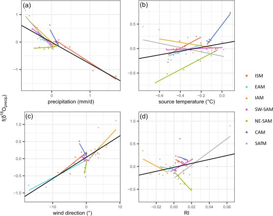
3.4 Multiple regression analysis of Holocene δ 18 Oprecip
The MLR analyses of simulated δ 18 Oprecip trends identify
the impact of an individual climate variable on δ 18 Oprecip in
the absence of changes in other variables. The global MLR
model includes the Holocene (1–9 ka) δ 18 Oprecip trends com-
bined across all monsoon regions (CAM, ISM, EAM, SW-
SAM, NE-SAM, SAfM, IAM). This global monsoon MLR
model has a pseudo-R 2 of 0.80 and shows statistically signif-
icant relationships between the anomalies in δ 18 Oprecip and
anomalies in regional precipitation, temperature and surface
Figure 3. Speleothem δ 18 O anomalies compared to anomalies of wind direction (Table 3). The partial residual plots (Fig. 6)
δ 18 Oprecip , precipitation and temperature from the ECHAM sim-
show there is a strong negative relationship with regional pre-
ulations for the (a) East Asian (EAM), (b) Indian (ISM) and
cipitation (t value of −8.75) and a strong positive relation-
(c) Indonesian–Australian (IAM) monsoons. The boxes show the
median value (line) and the interquartile range, and the whiskers ship (t value of 8.03) with surface wind direction over the
show the minimum and maximum values, with outliers represented moisture source region, an index of changes in either source
by grey dots. Note that the isotope axes are reversed, so that the area or moisture pathway. This indicates that increases in re-
most negative anomalies are at the top of the plot, to be consistent gional precipitation alone will lead to a decrease in δ 18 O,
with the assumed relationship with the direction of change in pre- whereas changes in source area and/or moisture pathway,
cipitation and temperature. in the absence of changes in other variables, will lead to a
significant change in δ 18 O. The relationship with tempera-
ture over the moisture source region is weaker, but positive
gions, except SW-SAM in the early Holocene. The EAM (t value of 2.05), i.e. an increase in temperature over the
and ISM regions (Fig. 4a–e) show the most positive δ 18 Ospel moisture source region will lead to an increase in δ 18 O if
z scores around 12 ka followed by a rapid decrease towards there are no changes in other climate variables. Precipitation
their most negative values at ∼ 9.5 and ∼ 9 ka respectively. recycling is not significant in this global analysis. The exact
The δ 18 Ospel z scores in the EAM are relatively constant from choice of source region has a negligible impact on the model
9.5 to ∼ 7 ka, whereas this plateau is present but less marked – for example, expanding the ISM source region to include
in the ISM. There is a gradual trend towards more positive the Bay of Bengal does not change the outcome of this anal-
δ 18 Ospel z scores towards the present in both regions there- ysis (Fig. S9, Table S1).
after. The SW-SAM records (Fig. 4i) have their most positive There are too few data points to make regressions for in-
δ 18 Ospel z scores in the early Holocene with a gradual trend dividual monsoon regions, but the distribution of data points
to more negative scores towards the present. By contrast, the for each region in the partial residual plots (Fig. 6) is indica-
IAM z scores (Fig. 4g) are most positive at 12 ka, gradually tive of the degree of conformity to the global MLR model
decrease until ca. 5 ka and are relatively flat thereafter. (representing the combined response across all monsoon re-
https://doi.org/10.5194/cp-17-1119-2021 Clim. Past, 17, 1119–1138, 20211128 S. E. Parker et al.: Interpreting speleothem records of monsoon changes Figure 4. Evolution of regional speleothem δ 18 O signals through the Holocene compared to δ 18 Oprecip simulated by the GISS model. Panels (a–e) show Northern Hemisphere monsoons (EAM denotes the East Asian monsoon; ISM denotes the Indian summer monsoon) and summer (May through September) insolation at 30◦ N (Berger, 1978). Panels (f–j) show Southern Hemisphere monsoons (SW-SAM denotes the southwestern South American monsoon; IAM denotes the Indonesian–Australian monsoon) and summer (November through March) insolation for 20◦ S (Berger, 1978). The speleothem δ 18 O changes are expressed as z scores, with a smoothed loess fit (3000-year window), and confidence intervals obtained by bootstrapping by site. δ 18 Oprecip values are expressed as anomalies from the pre-industrial control simulation. Note that the isotope axes are reversed, so that the most negative anomalies are at the top of the plot, to be consistent with the assumed relationship with the changes in insolation. Table 3. Results of the multiple linear regression analysis. Signifi- EAM and SW-SAM is broadly consistent with the overall cant relationships (P
S. E. Parker et al.: Interpreting speleothem records of monsoon changes                                                                 1129

Figure 5. Comparison of changes in summer insolation and δ 18 Ospel through the peak of the Last Interglacial (Marine Isotope Stage 5e)
from the (b, c) East Asian monsoon (EAM), (d, e) Indian summer monsoon (ISM), (g) southwestern South American monsoon (SW-SAM)
and (h) Indonesian–Australian monsoon (IAM) regions. The U–Th dates and uncertainties are shown for each record. The summer insolation
curves (Berger, 1978) are for May through September at 30◦ N in the Northern Hemisphere (a) and for November through March for 20◦ S
in the Southern Hemisphere (f). Note that the isotope axes are reversed, so that the most negative anomalies are at the top of the plot, to be
consistent with the assumed relationship with the changes in insolation. The LIG (Marine Isotope Stage 5e) time slice used in the analysis in
Sect. 2.4 is shown by the dark-grey bar.

4   Discussion                                                           tion dipole that exists between northeastern Brazil (Nordeste)
                                                                         and the continental interior (Berbery and Barros, 2002; Boers
We have shown that it is possible to derive an objective re-             et al., 2014). The anti-phasing of speleothem records from
gionalisation of speleothem records based on the PCoA of                 the two regions during the Holocene has been recognised in
the oxygen-isotope trends through the Holocene (Fig. 2).                 previous studies (Cruz et al., 2009; Deininger et al., 2019).
This approach separates out regions with a distinctive North-            The intermediate nature of the records from the maritime
ern Hemisphere signal (e.g. ISM, EAM, NE-SAM) from re-                   continent is consistent with the fact that the Indonesian–
gions with a distinctive Southern Hemisphere signal (e.g.                Australian (IAM) summer monsoon is influenced by cross-
SW-SAM, SAfM), reflecting the fact that the evolution of                 equatorial air flow and, hence, can be influenced by Northern
regional monsoons in each hemisphere follows, to some ex-                Hemisphere conditions (Trenberth et al., 2000). Palaeoenvi-
tent, insolation forcing. It also identifies regions that have           ronmental records from this region show mixed signals for
an intermediate pattern (e.g. IAM). The robustness of the re-            the Holocene: some have been interpreted as showing en-
gionalisation is borne out by the fact that Holocene compos-             hanced (Beaufort et al., 2010; Mohtadi et al., 2011; Quigley
ite trends from each region have tight confidence intervals              et al., 2010; Wyrwoll and Miller, 2001) and others reduced
(Fig. 4), showing that the signals of individual records across          precipitation (Kuhnt et al., 2015; Steinke et al., 2014) during
a region show broad similarities. The monsoon regions iden-              the early and mid-Holocene. Modelling studies have shown
tified by PCoA are consistent with previous studies (Wang                that this region is highly sensitive to SST changes in the
et al., 2014). The tracking of Northern Hemisphere insola-               Indian Ocean and South China Sea, which in turn reflect
tion is a recognised feature of monsoon systems in India                 changes in the Northern Hemisphere winter monsoons. Al-
and China (see reviews by Kaushal et al., 2018; Zhang et                 though most climate models produce a reduction in precipi-
al., 2019). The separation of speleothem records from NE-                tation across the IAM during the mid-Holocene in response
SAM from those in SW-SAM is consistent with the precipita-               to orbital forcing, this is less than might be expected in the

https://doi.org/10.5194/cp-17-1119-2021                                                                Clim. Past, 17, 1119–1138, 2021
1130 S. E. Parker et al.: Interpreting speleothem records of monsoon changes Figure 6. Partial residual plots from the multiple linear regression analysis, showing the relationship between anomalies in simulated δ 18 Oprecip and the four predictor variables, after considering the fitted partial effects of all the other predictors. The simulated δ 18 Oprecip values are anomalies relative to the pre-industrial control simulation and are annual values weighted by precipitation amount. The predictor variables are precipitation in the delineated monsoon region (mm d−1 ), temperature in the source region (◦ C), surface wind direction over the source region (◦ ) as an index of potential changes in source region and the ratio of precipitation recycling to total precipitation over the monsoon region (RI, unitless). The predictor variables are summer mean values, representing the summer monsoon, where summer is defined as May to September for the Northern Hemisphere monsoons and November to March for the Southern Hemisphere monsoons. absence of ocean feedbacks associated with changes in the India (Misra et al., 2019). The lagged response to increas- Indian Ocean (Zhao and Harrison, 2012). ing insolation is thought to be due to the presence of North- The separation of northern and southern monsoon regions ern Hemisphere ice sheets in the early Holocene (Zhang et is consistent with the idea that changes in monsoon rain- al., 2018). The persistence of wetter conditions through the fall are primarily driven by changes in insolation (Ding and early and mid-Holocene is thought to reflect the importance Chan, 2005; Kutzbach et al., 2008). Indeed, regional δ 18 Ospel of land surface and ocean feedbacks in sustaining regional composites from the EAM, ISM and SW-SAM show a clear monsoons (Dallmeyer et al., 2010; Kutzbach et al., 1996; relationship with the long-term trends in local summer in- Marzin and Braconnot, 2009; Rachmayani et al., 2015; Zhao solation (Fig. 4). Similar patterns are seen in individual and Harrison, 2012). The evolution of regional monsoons speleothem records from each region confirming that the during the LIG shows patterns similar to those observed dur- composite trends are representative. However, the compos- ing the Holocene, including the lagged response to insola- ite trends are not an exact mirror of the insolation signal over tion and the persistence of wet conditions after peak inso- the Holocene. For example, the ISM and EAM composites lation. This is again consistent with the idea that internal show a more rapid rise during the early Holocene than im- feedbacks play a role in modulating the monsoon response plied by the insolation forcing. The maximum wet phase in to insolation forcing. We have also shown that there is lit- these two regions lasts for ca. 3000 years, again contrasting tle difference in the isotopic values between the MH and the with the gradual decline in insolation forcing after its peak LIG in the ISM and EAM regions, which is also observed in at ca. 11 ka. Both the rapid increase and the persistence of individual speleothem records (Kathayat et al., 2016; Wang wet conditions for several thousand years is also observed in et al., 2008). The LIG (125 ka) period was characterised by other palaeohydrological records across southern and central higher summer insolation, higher CO2 concentrations (Otto- China, including pollen (Zhao et al., 2009; Li et al., 2018) Bliesner et al., 2017) and lower ice volumes (Dutton and and peat records (Hong et al., 2003; Zhou et al., 2004). Lambeck, 2012) than the MH, suggesting that the LIG ISM These features are also characteristic of lake records from and EAM monsoons should be stronger than the MH mon- Clim. Past, 17, 1119–1138, 2021 https://doi.org/10.5194/cp-17-1119-2021
S. E. Parker et al.: Interpreting speleothem records of monsoon changes                                                         1131

soons. The lack of a clear differentiation in the isotope sig-      ing drier conditions in the ISM, EAM and IAM, supported
nals between the LIG and MH suggests that other factors play        by simulated changes in δ 18 Oprecip and precipitation (Fig. 3).
a role in modulating the monsoon response to these forcings         Cooler SSTs of approximately 2 ◦ C (relative to the MH and
and may reflect the importance of global constraints on the         LIG) in the ISM and EAM and of approximately 3 ◦ C in IAM
externally forced expansion of the tropical circulation (Bia-       source areas, along with a ca. 5 % decrease in relative humid-
sutti et al., 2018).                                                ity (Yue et al., 2011), would result in a water vapour δ 18 O sig-
   Global relationships between δ 18 Oprecip and climate vari-      nal at the source that is ca. 1 ‰ more depleted than seawater.
ables (precipitation amount, temperature and surface wind           This depletion results from the temperature dependence of
direction; Fig. 6) are consistent with existing studies: a strong   equilibrium fractionation during evaporation and kinetic iso-
relationship with precipitation and a weaker temperature ef-        tope effects related to humidity (Clark and Fritz, 1997). This
fect have been widely observed at tropical and subtropical          fractionation counteracts any impact from enriched seawater
latitudes in modern observations (Dansgaard, 1964; Rozan-           δ 18 O values during the LGM (ca. +1 ‰ relative to the MH or
ski et al., 1993). The significant global relationship between      LIG; Waelbroeck et al., 2002). Cooler air temperatures will
δ 18 Oprecip and surface winds supports the idea that changes in    also result in a depletion of δ 18 Ospel during the LGM of ca.
moisture source and pathway are also important for explain-         0.4 ‰ and 0.6 ‰ for the ISM/EAM and IAM respectively, as
ing δ 18 O variability over the Holocene. The multiple regres-      a result of water–calcite (or water–aragonite) fractionation
sion analysis also provides insights into the relative impor-       (Grossman and Ku, 1986; Tremaine et al., 2011). This has
tance of different influences at a regional scale. In the ISM,      the effect of slightly reducing the regional LGM δ 18 Ospel sig-
the results support existing speleothem studies which sug-          nals, although the change is small and within the uncertainty
gest that changes in precipitation amount (Cai et al., 2015;        of the regional signals. Enriched δ 18 Oprecip and δ 18 Ospel val-
Fleitmann et al., 2004) and to a lesser extent moisture path-       ues during the LGM must therefore be caused by a signifi-
way (Breitenbach et al., 2010) drive δ 18 Ospel variability. The    cant decrease in atmospheric moisture and precipitation that
δ 18 O variability in the IAM region through the Holocene           resulted from the cooler conditions.
also appears to be strongly driven by changes in precipita-            We have used version 2 of the SISAL database (At-
tion and moisture pathway, consistent with the interpreta-          sawawaranunt et al., 2018; Comas-Bru et al., 2020a) in our
tion of Wurtzel et al. (2018). Changes in regional precip-          analyses. Despite the fact that SISALv2 includes more than
itation (where the cave sites are located) do not seem to           70 % of known speleothem isotope records, there are still too
explain the observed changes in δ 18 Ospel in the EAM dur-          few records from some regions (e.g. Africa, the Caribbean)
ing the Holocene, where Holocene δ 18 Oprecip evolution is          to make meaningful analyses. The records for older time pe-
largely driven by changes in atmospheric circulation (in-           riods are also sparse. For example, there are only 14 records
dexed by changes in surface winds). This is consistent with         from monsoon regions covering the LIG in SISALv2. Never-
existing studies that emphasise changes in moisture source          theless, our analyses show that there are robust and explica-
and/or pathway rather than local precipitation changes (Ma-         ble patterns for most monsoon regions during the Holocene
her, 2016; Maher and Thompson, 2012; Tan, 2014; Yang                and sufficient records to make meaningful analyses of the
et al., 2014). Speleothem δ 18 O records in the SW-SAM              LGM and LIG. Whilst there is a need for the generation of
clearly reflect regional-scale changes in precipitation, con-       new speleothem records from key regions such as northern
sistent with interpretations of individual records (Cruz et         Africa, further expansion of the SISAL database will cer-
al., 2009; Kanner et al., 2013). However, this is a region          tainly provide additional opportunities to analyse the evolu-
where changes in precipitation recycling also appear to be          tion of the monsoons through time.
important. Based on regional water budget estimates, recy-             The impact of age uncertainties, included in SISALv2, are
cling presently contributes ca. 25 %–35 % of the precipita-         not taken into account in our analyses. Age uncertainties dur-
tion over the Amazon (Brubaker et al., 1993; Eltahir and            ing the Holocene are smaller than the interval used for bin-
Bras, 1994); these figures increase up to ca. 40 %–60 % based       ning records and the width of the time windows used and,
on moisture tagging studies (Risi et al., 2013; Yoshimura et        thus, should not have a significant effect on our conclusions.
al., 2004).                                                         The mean age uncertainty at the LGM and LIG is ca. 430
   The LGM is characterised by lower Northern Hemisphere            and 1140 years respectively. However, varying the window
summer insolation, globally cooler temperatures, expanded           length for the selection of LGM and LIG samples from ±500
global ice volumes and lower GHG concentrations than ei-            to ±2000 years, thereby encompassing this uncertainty, has
ther the MH or the LIG. The MH and LIG (Marine Isotope              a negligible effect (< 0.5 ‰) on the average δ 18 O values.
Stage 5e) periods represent peaks in the present and last in-       Thus, the interglacial–glacial contrast in regional δ 18 Ospel is
terglacial periods, whereas the LGM represents maximum              also robust to age uncertainties.
ice extent during the Last Glacial Period. Hence, comparison           Isotope-enabled climate models are used in this study to
of these time periods provides a snapshot view of glacial–          explore observed regional-scale trends in δ 18 Ospel . There is
interglacial variability. The δ 18 Ospel anomalies are more pos-    a limited number of isotope-enabled models, and there are
itive during the LGM than during the MH or LIG, suggest-            no simulations of the same time period using the same ex-

https://doi.org/10.5194/cp-17-1119-2021                                                         Clim. Past, 17, 1119–1138, 2021
You can also read