Integrating Adaptation Expertise into Regional Climate Data Analyses through Tailored Climate Parameters
←
→
Page content transcription
If your browser does not render page correctly, please read the page content below
B      Meteorol. Z. (Contrib. Atm. Sci.), Vol. 28, No. 1, 41–57 (published online February 21, 2019)
       © 2019 The authors
                                                                                                                              Climatology

Integrating Adaptation Expertise into Regional Climate Data
Analyses through Tailored Climate Parameters
Janus Willem Schipper1,2∗ , Julia Hackenbruch2 , Hilke Simone Lentink2 and
Katrin Sedlmeier2,3
1
  South German Climate Office at Karlsruhe Institute of Technology, Germany
2
  Institute of Meteorology and Climate Research, Karlsruhe Institute of Technology, Germany
3
  Current affiliation: MeteoSwiss, Switzerland
(Manuscript received October 4, 2018; in revised form November 30, 2018; accepted December 14, 2018)

             Abstract
             Climate change affects many fields of action, ranging from city planning and forestry to agriculture and
             the tourism industry, for which climate adaptation is needed. Therefore, the main goal of the current study
             is to introduce a concept of how to integrate adaptation expertise into regional climate data analyses using
             so-called climate parameters. Latter describes a meteorological condition or threshold relevant to regional
             adaptation measures. To reach this goal, several steps were performed, starting with a survey and expert
             interviews on experiences of the climate influence on regional decision-making focusing on the State of
             Baden-Wuerttemberg in south-west Germany. After quantifying these experiences in terms of tailored climate
             parameters, they were analyzed using the observation datasets HYRAS and E-OBS as well as an ensemble of
             regional climate simulations for south-west Germany for a reference period (1971–2000) and the near future
             (2021–2050). Then, the relevance of the tailored climate parameters was described by a so-called “sensitivity
             assessment”. According to this assessment, the necessity for adaptation measures in a changing climate was
             identified for different fields of action. In the end, we show that a co-produced coupling of the expertise of
             climate scientists and decision-makers leads to a better understanding of the regional challenges of climate
             change and impacts. The results of the study show the high potential of tailored climate parameters through
             integrating practical knowledge into climate simulation analyses.
             Keywords: regional climate change, climate adaptation, decision-making, tailored climate parameters,
             observations, simulation ensemble

1 Introduction                                                                 (Schuster et al., 2017), but also by how heat is experi-
                                                                               enced (Kunz-Plapp et al., 2016). Storm surges or heavy
                                                                               rain and flash floods affect spatial planning (Rannow
Weather and climate influence our daily life in different
                                                                               et al., 2010), the frequency of snow days affects win-
fields of action, as there are e.g. city planning, forestry,
                                                                               ter tourism (Endler and Matzarakis, 2011b) and the
agriculture, and the tourism industry (Pachauri et al.,
                                                                               heat stress and sultry conditions affect summer tourism
2014). Whereas weather acts on short term time scales
                                                                               in general (Endler and Matzarakis, 2011a) and, e.g.
of up to ten days, the impact of climate is noticeable over
                                                                               the number of zoo visitations by tourists, in particular
time scales of several decades and longer (e.g. Hurrell
                                                                               (Hewer and Gough, 2016). For viticulture this may
et al., 2009; Meehl et al., 2009). The same applies for
                                                                               result in late frost damage risk (Molitor et al., 2014),
decision-making processes in municipalities and compa-
                                                                               an increase in water demand due to higher evaporation
nies; on the short term, for example heat waves and ex-
                                                                               because of higher temperatures (Ramos et al., 2008), or
treme precipitation events influence decisions to provide
                                                                               negative changes in freshness and color (Drappier et al.,
enough drinking water or evacuate people from regions
                                                                               2017).
at risk, respectively. On the long term, however, climate
change may alter many of these short term influences                              As climate change is advancing, climate adaption,
over decades. Health impacts on persons caused by ex-                          especially on the regional scale, comes more into focus
treme events increase, for example, because of longer                          (IPCC, 2013b). Here, we refer to climate adaptation as
and more intensive heat waves in summer, resulting                             “the process of adjustment to actual or expected climate
in heat-stress related morbidity and mortality (Schus-                         and its effects” (Field et al., 2014, p. 40).
ter et al., 2014; Scherer et al., 2013). Especially, heat                         Climate scientists usually have little in-depth knowl-
waves in cities have a major impact on the health of                           edge about many of the day-to-day procedures in
its citizens, not only caused by their physical fitness                        decision-making relating to climate adaptation, as they
                                                                               have their expertise mainly in climate observations and
∗
 Corresponding author: Janus Willem Schipper, South German Climate Of-         simulations. Also, different perceptions about the ur-
fice at Karlsruhe Institute of Technology, Germany, e-mail: schipper@kit.edu   gency to adapt to climate change between scientists and

                                                                                                                           © 2019 The authors
DOI 10.1127/metz/2019/0878                                     Gebrüder Borntraeger Science Publishers, Stuttgart, www.borntraeger-cramer.com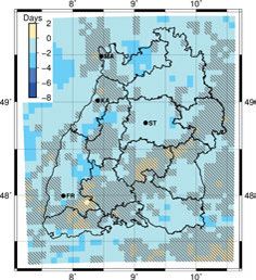
42                        J.W. Schipper et al.: Tailored Climate Parameters                      Meteorol. Z. (Contrib. Atm. Sci.)
                                                                                                                         28, 2019

decision-makers exist (Runhaar et al., 2012). More-                ing by decision-makers concerning adaptation planning
over, regional climate models were not intended to pro-            in e.g. urban planning, health care, forestry, and agri-
vide climate information or data requests by munici-               culture. However, this is not always the case, as was
palities, companies or other scientific disciplines from           shown by a survey conducted by the South German Cli-
the start. Consequently, this information is not neces-            mate Office at the Karlsruhe Institute of Technology in
sarily part of the standard output of regional climate             the State of Baden-Wuerttemberg, Germany (Hacken-
simulations (Hackenbruch et al., 2017). Even though                bruch et al., 2017). Therefore, in order to integrate prac-
the development in the field of regional climate simu-             titioners’ experience in the post-processing of regional
lations has shown a large improvement compared to ob-              climate simulation results, specific parameters should be
servations during the last decades, practitioners (like e.g.       built, which describe the climatological part of a deci-
city administrations or companies) still often need spe-           sion making process. They can be combinations of pa-
cific information that can be integrated into their deci-          rameters, like precipitation and temperature, or specific
sions. Hence, two processes are essential. First, gath-            threshold exceedances of single parameters, each tai-
ering information about the impact of climate change               lored to the individual needs of the practitioners. Also
on decision-making by a direct communication between               durations of certain weather situations have to be con-
scientists and experts from outside science. Climate ser-          sidered, for example periods of very dry or very warm
vices try to coordinate this process, as it is one of their        weather. The development of these so-called tailored cli-
tasks to communicate between science and society. The              mate parameters builds the basis for the user-oriented
second process is to accurately simulate the regional cli-         analyses of regional climate model simulations in the
mate to provide reliable data.                                     current study.
    Yet, combining these processes of science and so-                  Hence, the main goal was to proof the concept of co-
ciety, which is generally called “coproducing of usable            producing information for climate adaptation measures
climate science” (Wall et al., 2017) is tricky. There are          by using tailored climate parameters. The current paper
several reasons for this. One reason is the “lack of high-         shows the potential of a direct integration of experts’ ex-
resolution data for the local level in combination with            perience into climate simulation post-processing analy-
actor-specific characteristics” (Lehmann et al., 2015).            ses by presenting a small selection of tailored climate
Also, decision-makers, often rely on individual experi-            parameters, all relevant in (parts of) south-west Ger-
ence for their communication, which is not necessarily             many. As the individual experts only represented their
based on scientific evidence (Cvitanovic et al., 2015).            field of action, the results in the current paper only have
    One way to increase the understanding between sci-             a narrative character. From the list of parameters defined
entists and stakeholders is the use of climate indicators.         together with the experts in this paper, the process is ex-
Such indicators for climate and climate change are de-             emplary discussed for four climate parameters: salting
scribed and presented in numerous printed and online               days, warm and dry summers, years between warm
climate atlases (e.g. Royal Netherlands Meteorological             and dry summers, and hiking days. The parameters
Institute (KNMI), 2018; NOAA, 2018; Prairie Cli-                   use different climatological definitions, target different
mate Centre, 2016; Meinke et al., 2010; DWD, 2009).                audiences, and have different implications. The defini-
These atlases hold many meteorological parameters as               tion of the parameters will be described in the results
well as deduced parameters for specific applications,              (section 3), the according fields of application in south-
e.g. water management (IWMI, 2009), trees (Prasad                  west Germany are briefly presented in the following.
et al., 2007), and birds (Matthews et al., 2007). Most
of these atlases are set up either from a particular point         Salting days
of view using the experience from practitioners or from
a meteorological point of view based on (climatological)           As climate change evolves, strategic planning of win-
limits and thresholds. Classical climatological statistics         ter road maintenance is of increasing importance
like annual precipitation sums, mean temperatures or               (Matthews et al., 2017). Concerning winter time, sev-
derived statistics generally reflect the past and the fu-          eral indices exist to detect the severity of a winter
ture climate from a meteorological point of view very              season. For example, the Accumulated Winter Sea-
well. Examples are summer days (maximum tempera-                   son Severity Index (AWSSI) includes temperature av-
ture ≥ 25 °C), frost days (minimum temperature < 0 °C),            erages and extremes, snowfall totals, and snow depth
maximum number of consecutive dry days (precipita-                 (Boustead et al., 2015). With respect to winter services,
tion < 1 mm), cold-spell duration index, and heavy pre-            the annual amount of days to salt the road is depen-
cipitation days (precipitation ≥ 10 mm), which are all             dent on the temperature of the road and is difficult to
widely used (e.g. Royal Netherlands Meteorological In-             quantify (Missenard, 1933). As winter services very
stitute (KNMI), 2018). Such indicators are very useful             much depend on the state of the weather, the so-called
for monitoring climate change, making the topic more               Hulme-index was developed, which includes road sur-
transparent for science and stakeholders (ETCCDI – Ex-             face temperature, days with snow on the ground, and
pert Team on Climate Change Detection and Indices;                 frost days (Hulme, 1982). However, besides meteoro-
Peterson, 2005; Karl et al., 1999). Ideally, these in-             logical aspects, personnel planning, modification of ve-
dicators also hold information relevant for action tak-            hicles, and the purchasing of salt are important criteria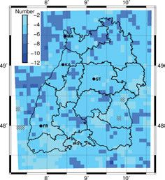
Meteorol. Z. (Contrib. Atm. Sci.)                   J.W. Schipper et al.: Tailored Climate Parameters                  43
28, 2019

for winter service planning (Venäläinen and Kangas,            younger trees are able to recover better than smaller and
2003). For example, a study among winter services in           older trees (Zang et al., 2014). In combination with the
Denmark showed that the costs for the purchase of salt         tailored climate parameter warm and dry summers, this
can vary much regionally as a consequence of the length        parameter gives a good indication about the stress for
of the salt routes (Knudsen, 1994). The current study          forests in climate change.
adds a climate parameter describing the meteorological
part of the decision whether to salt or not, based on the      Hiking days
experience of consulted winter services.
                                                               For the State of Baden-Wuerttemberg, tourism is an im-
                                                               portant field of action, dominated by people going hik-
Warm and dry summers                                           ing, especially for the higher elevated areas. In partic-
During warm and dry summers, people, animals, and              ular, the practical relevance of hiking days lies in the
plants can be affected by heat stress. As green spaces         concern of the tourism industry by finding out if the
have a positive psychological effect, especially in cities,    number of hikers will increase or decrease due to cli-
dried out areas can have a negative effect on the well-        mate change. A change in hiking days may involve a
being of humans, leading to a higher mortality (Scherer        change of priorities in areas already or not yet made ac-
et al., 2013). Besides, it is suggested that elderly people    cessible to hiking. Several climate studies already exist
more often lack to perceive themselves as vulnerable to        in the field of tourism, in which the necessity for climate
heat than younger people do (Kunz-Plapp et al., 2016;          adaptation and the lack of the implementation of adapta-
Großmann et al., 2012). This leads to a strong depen-          tion measures is for example related to the unpredictabil-
dency of mortality and age, which was found in the ex-         ity of the future climate (Endler and Matzarakis,
ceptionally long and warm heat wave in Central Europe          2011a; Weaver, 2011). Among these studies, it is dis-
2003 (Fouillet et al., 2006). During this extremely hot        cussed, that the type of tourism alters, depending on the
and dry summer (Schär et al., 2004), the total heat-           change of temperatures due to climate change in Ger-
related death toll was about 70 000 (Robine et al., 2008).     many (Hamilton and Tol, 2007). More specifically,
Meteorological observations throughout Europe over the         indices, like e.g. a Comfort Index (Grillakis et al.,
last about 100 years show an increase of dry summers,          2016), are generated to identify the sensitivity of sum-
which has mainly to do with the increase of temperature        mer tourism to increasing temperatures. A review cover-
(Briffa et al., 2009). The situation concerning precip-        ing the impact of climate change on the tourism industry
itation is not that clear. For example, models expect a        and the potential of adaptation emphasized the necessity
decrease of mean precipitation, but more intense heavy         of community-based research (Kaján and Saarinen,
and extreme rainfalls in Central Europe in future dur-         2013). The newly developed tailored climate parameter
ing summer (Rajczak and Schär, 2017). Orth et al.              in the current study takes into account the hiking behav-
(2016) also state that the drying trend for Central Europe     ior in the field of tourism.
will continue in future and possibly be even stronger              A description of the data and the method used can
than is expected by the model ensemble of the 5th As-          be found in section 2, whereas the results are described
sessment Report of the IPCC. In forestry, an increase in       in section 3. Finally, the discussion and conclusions are
warm and dry summers could intensify the development           presented in section 4.
of the so-called bark and wood boring beetles, mainly in
elderly, predominantly weaker, trees. However, the inter-      2 Data and method
actions between the beetles and the trees associated with
their microbial community are not yet sufficiently un-         2.1 Data
derstood to give a final conclusion (Sallé et al., 2014).
Nevertheless, a world wide study about the extent of for-      The study region covered the federal state of Baden-
est area in dry-land habitats showed through a photo-          Wuerttemberg in south-west Germany including neigh-
interpretation approach using large databases of satellite     boring areas (Figure 1a) with the dimensions in east-
imagery that the area of dry-lands is larger than previous     west direction of 359 km (southern border) and 378 km
estimates (Bastin et al., 2017). The current study uses        (northern border) and in north-south direction of 283 km
the experience in the fields of forestry and pomiculture       (western border) and 280 km (eastern border). It is, on
to develop a new tailored climate parameter related to         the one hand, characterized by a pronounced orography
warm and dry summers.                                          with the lowlands of the Rhine Valley in the West (about
                                                               200 m asl.), the low mountain ranges Black Forest and
Years between warm and dry summers                             Swabian Jura in the center (up to 1,000 m asl.), and parts
                                                               of the Alps in the south-east (above 2,000 m asl.) and
As trees need several years to recover from a warm             corresponding climates. On the other hand, the area is
and, primarily dry summer, trees show the consequences         very heterogeneous with respect to land use and popula-
even after three years, depending on the tree species          tion density, with the rural, forested regions of the moun-
(Pretzsch et al., 2013). Also, the time period for a           tain ranges and the densely populated areas in the river
tree to recover depends on its size and age; larger and        valleys, with the cities of Karlsruhe, Mannheim, and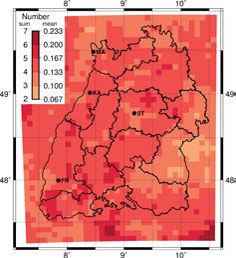
44                          J.W. Schipper et al.: Tailored Climate Parameters                       Meteorol. Z. (Contrib. Atm. Sci.)
                                                                                                                            28, 2019

Figure 1: Study region and the State of Baden-Wuerttemberg. (a) Geographical location within Germany and Europe. (b) Topography
according to the Global Elevation Data ETOPO2 (NGDC, 2010). Black lines – and the black lines in the following similar maps – denote
the regions in Baden-Wuerttemberg used in the sensitivity assessment.

Freiburg in the Rhine Valley and the metropolitan region             institutions to reach a representative group of partici-
Stuttgart in central Baden-Wuerttemberg (Figure 1b).                 pants.
   The current study used three data sources, which                      The 32 interviewees of the expert interviews, includ-
are Experts’ experience, Observations, and Climate                   ing the one enterprise, were selected to cover many
simulations. Depending on the data needed during the                 fields of action. Therefore, the focus was on the nine
steps in the current study, the according data source was            fields of action of the 2015 adopted adaptation strat-
chosen, which is described in the following in more                  egy of the Ministry of the Environment, Climate Protec-
detail.                                                              tion and the Energy Sector Baden-Wuerttemberg, which
                                                                     are forestry, agriculture, soil, nature protection, water
Experts’ experience                                                  economy, tourism, health, urban and land use planning,
The first data source contained the experience about                 and the economic and energy sectors (Ministerium für
the role of the climate in day-to-day action of munic-               Umwelt, Klima und Energiewirtschaft, 2015). The
ipalities, enterprises, and further experts. It was based            questions were closely related to the questionnaire sur-
on a questionnaire survey among municipalities (Hack-                veys. Because of the possibility of further questions, the
enbruch et al., 2017), a questionnaire survey among                  dynamical process of the interviews was quite effective.
private enterprises, and semi-standardized expert inter-             Each time experts are mentioned in the current study, the
views. Both surveys and the expert interviews focused                experts from the expert interviews as well as the respon-
on the State of Baden-Wuerttemberg. The surveys en-                  dents from the surveys are meant.
compassed 26 closed and open-ended questions and
were subdivided into four sections: “state of adaptation”,           Observations
“relevant weather events or climate variables concern-
ing adaptation”, “the sensitivity to climate change”, and            The second data source contained meteorological obser-
“the location and the information sources of the respon-             vations that were based on two observational data sets
dents”. The survey among municipalities was distributed              (Table 1). The observational data set HYRAS (“HYdrol-
by the Baden-Wuerttemberg Council of Cities to its 180               ogische RASterdaten”) has a spatial resolution of ∼5 km
members, which represent a cross-section of the mu-                  and it contains the parameters daily mean temperature
nicipalities in Baden-Wuerttemberg. In total, 23 munic-              and daily precipitation sum for roughly Germany (Frick
ipalities responded, corresponding to about 13 %, which              et al., 2014; Rauthe et al., 2013). The spatial resolution
is comparable to similar studies (e.g. Martinez and                  of HYRAS is close to the resolution of the model simu-
Bray, 2014). The survey among private enterprises was                lations of ∼7 km – which was decided to be the resolu-
distributed by the State Office for the Environment,                 tion of interest in the current study –, so the data set was
Measurements and Nature Conservation of the Federal                  bilinearly interpolated onto the model grid. As HYRAS
State of Baden-Wuerttemberg (LUBW) and reaches the                   does not contain information about daily maximum and
majority of larger enterprises in Baden-Wuerttemberg.                minimum temperature, the high-resolution gridded data
Unfortunately, only one enterprise responded from this               set of daily climate over Europe, E-OBS, was addition-
survey, wherefore it was added to the list of experts, hav-          ally used (Haylock et al., 2008). It has a spatial resolu-
ing an individual interview. Although the authors did not            tion of ∼24 km, therefore, it was, after being bilinear in-
get direct access to the addresses of the survey lists, be-          terpolated onto the model grid, also height corrected us-
cause of data privacy matters, they were assured by both             ing the orography from the model simulations. Both ob-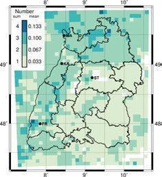
Meteorol. Z. (Contrib. Atm. Sci.)                                J.W. Schipper et al.: Tailored Climate Parameters                       45
28, 2019

Table 1: The observational data sets HYRAS (Frick et al., 2014; Rauthe et al., 2013) and E-OBS (Haylock et al., 2008) as well as the
regional climate model simulations data set COSMO-CLM (Sedlmeier, 2015) with the corresponding variables, time periods, and original
spatial resolution.

                                             variables                                  time periods           original resolution
        data set             Pday,sum   T day,mean   T day,min     T day,max    1971–2000      2021–2050   temporal         spatial
        observations
                  HYRAS         X          X                                        X                        daily     ∼5 km (0.045°)
                   E-OBS                                 X            X             X                        daily     ∼24 km (0.22°)
        model simulations
         COSMO-CLM*             X          X             X            X             X                  X    hourly     ∼7 km (0.0625°)
        *Ensemble containing twelve members (for details, see Table 2)

servational data sets cover the climate period 1971–2000                       ensemble projects such as ENSEMBLES (spatial reso-
(reference period) at a temporal resolution of one day.                        lution: ∼25 km; van der Linden and Mitchell, 2009)
                                                                               or CORDEX (spatial resolution: ∼11 km; Giorgi et al.,
Model simulations                                                              2009) have a higher number of members and there-
                                                                               fore might yield a more realistic representation of un-
The third data source was a regional climate ensem-                            certainty (but still not span the full range). However, as
ble with the regional climate model COSMO-CLM,                                 this study is more a proof of concept, we opted for us-
version 4.8 (Table 1) containing twelve climate sim-                           ing the ensemble with the highest available spatial res-
ulations (Sedlmeier et al., 2018; Sedlmeier, 2015).                            olution (to the authors’ knowledge – Sedlmeier et al.,
It was generated at the Institute of Meteorology and                           2018) for our study region at the moment of study,
Climate Research, Department Tropospheric Research                             which was 0.0625° (∼7 km), covering the climate peri-
(IMK-TRO), of the Karlsruhe Institute of Technol-                              ods 1971–2000 (reference period) and 2021–2050 (near
ogy (KIT). COSMO-CLM is the climate version of the                             future). The temporal resolution was one hour, which
operational weather forecasting model of the German                            was aggregated to one day for the current work. From
Weather Service (COnsortium for Small scale MOdel-                             the climate sciences’ perspective, the increasing spa-
ing in CLimate Mode – Rockel et al., 2008; Steppeler                           tial resolution of regional climate models compared to
et al., 2003). At the time of the study, there were no re-                     global models allows a better representation of meteoro-
gional climate simulations available for other emission                        logical variables, like temperature and precipitation, on
scenarios at this high spatial resolution for the study re-                    a regional scale (e.g. Fosser et al., 2015; Feldmann
gion. Also, as experts were asked to tell their experience                     et al., 2013), and enables a direct use for impact stud-
in their specific region, the assignment to their region                       ies (Hackenbruch et al., 2016). The improvement of
was necessary, which can best be done at a high spa-                           the spatial and temporal variability of the meteorologi-
tial resolution. The ensemble was generated by taking                          cal variables leads to a better representation of extreme
the results of different global climate models (some with                      events, predominantly due to a more accurate represen-
different realizations) as initial and boundary conditions                     tation of surface and orography fields (e.g. Panitz et al.,
as well as using the atmospheric forcing shifting method                       2015; Prein et al., 2015; Knote et al., 2010). Other
(Sasse and Schädler, 2014). The global climate mod-                            variables, like e.g. local convection, large scale circu-
els were forced by the greenhouse gas emission scenar-                         lation, and storm tracks, were not focus of the current
ios A1B (Nakicenovic et al., 2000) and RCP8.5 (Moss                            study, as they were not mentioned by the experts.
et al., 2010) for the near future. However from two dif-
ferent “emission scenario families”, both emission sce-                            In order to correct for systematic differences be-
narios show a similar course between 2021 and 2050,                            tween the model simulation results and the observa-
which is at the upper limit of the scenario spectrum                           tions, the ensemble was bias corrected for the four vari-
(Keuler et al., 2016; Pfeifer et al., 2015; Jacob et al.,                      ables listed in Table 1, using the corresponding avail-
2014). According to observations, these scenarios seem                         able observational data sets before calculating the cli-
to reflect the current development of greenhouse gas                           mate parameters. The bias correction was needed to cor-
emissions realistically (Sedlmeier et al., 2018). As the                       rect for the cold bias at temperature and the underesti-
future time period 2021–2050 is relatively close to the                        mating of the number of dry days generally simulated
current climate, the ensemble spread originates predom-                        by COSMO-CLM, especially considering extreme val-
inantly from the driving global models, rather than from                       ues. Sedlmeier (2015) stated that this correction can
the emission scenarios (Sedlmeier, 2015).                                      have an effect on the climate change signal and should
    Note, that the ensemble used in the current study                          therefore kept in mind when interpreting the magnitude
has twelve members, only (Table 1). Therefore, it most                         of the climate change signal.
likely does not include the full uncertainty range cov-                           Daily precipitation sum (Pday,sum ) and daily mean
ered by larger ensembles. Large regional climate model                         temperature (T day,mean ) were corrected using a simple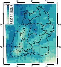
46                           J.W. Schipper et al.: Tailored Climate Parameters                         Meteorol. Z. (Contrib. Atm. Sci.)
                                                                                                                               28, 2019

Table 2: An overview of the members of the ensemble. The regional model is COSMO-CLM (version 4.8). All model simulations existed
for the reference period (1971–2000) and the near future (2021–2050) (IPCC, 2013a). A detailed description of the ensemble can be found
in Sedlmeier (2015).

                           Global models           Future climate scenarios      Sources
                           CGCM3.1                 A1B                           Scinocca et al. (2008)
                           CNRM-CM5                RCP8.5                        Voldoire et al. (2013)
                           ECHAM5-r1               A1B                           Roeckner et al. (2003)
                           ECHAM5-r2               A1B                           Roeckner et al. (2003)
                           ECHAM5-r3               A1B                           Roeckner et al. (2003)
                           ECHAM6                  RCP8.5                        Stevens et al. (2013)
                           ECHAM6-AFS-E2           RCP8.5                        Sasse and Schädler (2014)
                           ECHAM6-AFS-N2           RCP8.5                        Sasse and Schädler (2014)
                           ECHAM6-AFS-S2           RCP8.5                        Sasse and Schädler (2014)
                           ECHAM6-AFS-W2           RCP8.5                        Sasse and Schädler (2014)
                           EC-EARTH                RCP8.5                        Hazeleger et al. (2010)
                           HadGEM2-ES              RCP8.5                        Collins et al. (2011)

additive/multiplicative correction based on monthly val-
ues (BCM and MCA in Berg et al., 2012), daily mini-
mum and maximum temperature (T day,min and T day,max ,
resp.) by quantile mapping (e.g. Li et al., 2010).

2.2 Method
The method to reach the goals of the current study con-
sists of four steps (Figure 2). The first step was to sum-
marize the answers of the surveys as well as the inter-               Figure 2: Methodic four-step-approach to generate tailored climate
                                                                      parameters and evaluate their sensitivity.
views and deduce the information indicated as relevant
by the experts for climate change adaptation in Baden-
Wuerttemberg. From this information, events were iden-                with the model simulation results were made to gain
tified, closely related to the past experience of the stake-          confidence in the model simulations. Generally, it was
holders and having a potential impact on future deci-                 found that the used models simulated the observations
sions and usually contained statements like “at colder                quite well, as will be shown for the individual climate
temperatures”, “not too much rain”, or “not too dry                   parameters in the results section later on. The model
for a long period”. To get fixed climate parameters, we               simulation results for the period 2021–2050 were used
harmonized the experience of the experts with realistic               to calculate the possible future change for each tailored
boundaries from a meteorological point of view. As was                climate parameter. The statistical significance of future
to be expected, most experts had difficulties to give in-             changes in the tailored climate parameters was tested us-
formation about how to design tailored climate parame-                ing the paired Wilcoxon rank sum test on the simulated
ters, when first asked. The given answers included e.g.               differences of the 30-year mean (or sum) in the ensem-
“Until now, we never thought about tailored climate pa-               ble at each single grid point (Wilks, 2011). In detail, this
rameters, but it sounds interesting to do so.’’ (translated           means that the differences between twelve values (the
from the original quote in German language). That is                  size of the ensemble) for the reference period and the
why in reality, it was a highly iterative process, with               near future were tested on the 95 %-significance level
close cooperation between the experts and the climate                 for the magnitude and the leading sign of the changes
scientists. These fruitful discussions formed the basis of            for each grid point. The test is in accordance with the
the current study.                                                    approach for testing climate change signals used in the
    In the end, the statements described definitions of               fifth assessment report of the IPCC (IPCC, 2013a). Grid
e.g. the exceedance of specific temperature limits or                 cells not showing a significant changed are hatched in
precipitation amounts, and periods of extreme weather                 all maps.
as well as combinations of those, all closely related to                  The third step in the current work was to point
adaptation consideration. These definitions are called                out the relevance of the tailored climate parameters for
tailored climate parameters, from now on.                             adaptation measures. Therefore, fact sheets of about two
    In the second step, the tailored climate parameters               to three pages were prepared. They contained first maps
were calculated for each single grid point in the study re-           and graphs with the results of the tailored climate param-
gion for the observations and each individual ensemble                eters, using the available observations as well as simu-
member from daily data for the time period 1971–2000.                 lation results. Additionally, the climatology of the pa-
Comparisons between the results from the observations                 rameters was described and a summary of the impacts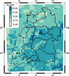
Meteorol. Z. (Contrib. Atm. Sci.) J.W. Schipper et al.: Tailored Climate Parameters 47
28, 2019
Table 3: Sensitivity assessment described by three categories of under the given limits from the third step. It should be
climate adaptation measures corresponding to a traffic light. noted that this part of the current study had its focus on
Baden-Wuerttemberg, only, because the experts origi-
climate adaptation nated from this state. Therefore, the maps holding the
categories need costs sensitivity of the climate parameters can only be shown
• red strong high for (part of) the state of Baden-Wuerttemberg. In the
• yellow medium medium end, part of the results were published in a brochure,
• green no or little no or low which was distributed among the experts (Schipper
et al., 2017).
of the climate parameters on the specific field of actions 3 Results
was given. These fact sheets were communicated to the
respective experts and formed the basis for a direct re- The approach of integrating adaptation expertise into re-
action of the experts on their tailored climate parame- gional climate simulation analyses is exemplarily shown
ters. Especially for the observations, it was vital to know, based on a selection of four tailored climate parame-
if the calculated values of the tailored climate param- ters: salting days, warm and dry summers, years be-
eters within Baden-Wuerttemberg agreed with the ex- tween warm and dry summers, and hiking days, all
perts’ experience. Also, the experts gave feedback about based on the experience of experts in the State of Baden-
the impact of the changes of the tailored parameters Wuerttemberg. The framework in which the parameters
on adaptation measures from their experience. That is, have their impact was already discussed in the introduc-
which adaptation measures are supposed to be realized tion. For each of the four climate parameters, the results
at what future changes of the parameters. This is what of the four steps mentioned in the methods section are
we call “sensitivity assessment” in this context and is discussed. It should be noted that all climate scenar-
also in accordance with IPCC definitions (IPCC, 2013a). ios are based on an ensemble containing twelve simu-
Note, that the sensitivity assessment in this context is not lations as described above, which most likely does not
mentioned to reflect the robustness or reliability of the span the whole uncertainty range. However, the main
model results. The sensitivity assessment was very chal- focus of this study is to introduce the concept of in-
lenging for the experts. Although many experts could tegrating expert knowledge to co-design tailored cli-
tell in detail about their experience in the past, they com- mate information for adaptation purposes. Integrating
monly had difficulties in, first, quantifying their experi- large regional downscaling experiments (such as e.g.
ence at all and, second, defining limits for this quantifi- CORDEX – http://www.cordex.org/) is left for further
cation corresponding to concrete adaptation measures. studies.
In detail, for the sensitivity assessment of a specific
tailored climate parameter, the experts assigned the re- 3.1 Salting days
sults of the parameter to a category, corresponding to the
colors of a traffic light (Table 3). If a climate parameter Winter services stated that favorable weather conditions
was assigned to the green category, there is no or little for salting roads (“salting days” in the following) de-
need for climate change adaptation, which is associated pend on temperature and precipitation, from a meteoro-
with no or low costs. If a tailored climate parameter was logical point of view. The definition in detail says that
in the yellow category, there is a medium need for cli- for a salting day the minimum temperature of that day
mate adaptation. This corresponds to rather easy to im- should not exceed 2 °C, while the precipitation sum is at
plement measures and medium costs. The red category least 0.5 mm (equation 3.1).
means a strong need for adaptation, with complex mea- ⎧
sures necessary, causing high costs. The experts were ⎪
⎪
⎪0
⎪
⎨
asked to assign one of the categories (green, yellow, or salting day = ⎪
⎪1, T day,min ≤ 2 [°C] and (3.1)
red) to the status of the tailored climate parameter dur- ⎪
⎪
⎩ Pday,sum ≥ 0.5 [mm]
ing the reference period, as well as to estimate at what
threshold the climate parameter would change its cate- In equation 3.1, T day,min and Pday,sum denote the daily
gory. The thresholds could be given in absolute as well minimum temperature and daily precipitation sum, re-
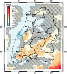
as in relative numbers. spectively. The observations show a higher number of
As a fourth and last step, the categories were cal- salting days per year at higher elevations – up to around
culated and displayed for the observations in maps to 100 days – compared to between 20 and 40 days in the
gain a spatial overview of the extent of the impact of the Rhine valley (Figure 3a). This means that higher ele-
investigated climate parameters (Figure 2). For the fu- vated areas need salting during more or less the entire
ture development of the climate parameters, a change in winter season.
color-coding was carried out for each grid cell for which A decrease is expected from the regional climate
more than six simulations (which is more than 50 % of simulation ensemble mean for each grid cell of between
the maximum available simulation runs) exceeded or go two and twelve days within the study region (Figure 3b).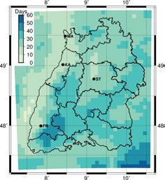
48                        J.W. Schipper et al.: Tailored Climate Parameters                           Meteorol. Z. (Contrib. Atm. Sci.)
                                                                                                                              28, 2019

              (a)                           (b)
Figure 3: Average number of days with favorable weather con-
ditions for salting (salting days) per year. (a) Observations
(1971–2000). (b) Mean expected annual changes from model sim-      Figure 4: Inter-annual variability (spatial average) of the number
ulations for 2021–2050 compared to 1971–2000.                      of days with favorable weather conditions for salting in each model
                                                                   simulation (Table 2) for the reference period and the observations
This is mainly due to the projected future temperature             (1971–2000, left panel) and the near future (2021–2050, right panel).
increase, because of global climate change, on which               A cross denotes one year, a white circle the average value over the
the salting days are largely dependent. The decrease of            corresponding period. The black lines denote the average value over
                                                                   all models and all years in the corresponding period. A star (*) at
salting days is almost uniform with a little less decrease
                                                                   a model name at the right panel (near future) denotes a significant
in higher elevated areas.                                          change compared to the reference period for that particular simula-
    The number of salting days of the spatial averaged             tion run.
ensemble mean is 52.1 days per year during the refer-
ence period, which is very close to the observations with
49.4 days per year (Figure 4). Also, the simulated stan-           ern part of the study region do not change significantly
dard deviation, as an indicator for the annual variability         (hatched areas).
of the number of salting days, of the simulation ensem-                The number of salting days, which are part of a clus-
ble is close to the observed standard deviation (9.2 days          ter of two to five days, occur more often and are region-
and 10.1 days, resp.). The standard deviation for the near         ally more differentiated than for the single stand-alone
future slightly decreases to 9.0 days. The expected de-            days (Figure 5b). At higher elevations, up to 50 days are
crease of salting days per year for the ensemble mean              part of such cluster lengths, which corresponds to be-
and averaged over the study region is 7.8 (from 52.1               tween ten and 25 clusters per year. In contrast, below
to 44.3 days). The largest expected decrease of a sin-             20 days are counted in the Rhine Valley, which corre-
gle simulation run was 11.2 days per year (from 54.8               sponds to between four and ten clusters per winter. The
to 43.6 days), initiated by the global climate model EC-           smallest numbers occur in the northern part of the study
EARTH. In contrast, the smallest decrease was 2.7 days             region with ten to 15 salting days within the cluster of
per year (from 50.4 to 47.7 days), initiated by the global         two to five days. The decrease of these days is generally
climate model ECHAM5-r3. The change of the median                  expected to be larger than for the single stand-alone days
is significant for each single simulation run.                     (Figure 5e).
    Concerning winter services, experts stated, that for               Salting days that are part of clusters of six days and
planning purposes, it makes a difference whether the               more are rather seldom in the study region (Figure 5c).
salting days are evenly distributed over single days dur-          The observed number of days of up to 20 corresponds
ing winter time or are clustered in larger periods of con-         to about three clusters of six days per winter and even
secutive days. Therefore, we additionally looked into de-          less for longer clusters. An exception are the higher
tail at the number of salting days in three selected clus-         elevations in the Black Forest and the Alps with up to
ters: single stand-alone days, two to five days, and six           40 days, corresponding to a maximum of six clusters of
days and longer (Figure 5). Note, that we counted the              six days or longer per year. The decrease of the number
number of days being part of a selected cluster, rather            of salting days within this cluster length in the near
than the number of clusters. This was done to enable a             future compared to the reference period is rather small as
direct comparison between the different cluster lengths.           well and not significant in about 63 % of the study region
    The average number of single stand-alone days per              (Figure 5f). Note, that for the salting days in the single
year is about 13 days in the reference period (Fig-                clusters the difference in weather conditions is highly
ure 5a). With a minimum and maximum value of 9.8 and               varying between single years as well as for the salting
15.6 days, resp., regional differences are rather small.           days in total.
According to the simulations, these single days are ex-                Regarding the sensitivity assessment, experts from
pected to decrease for the ensemble mean and spatial av-           the administrative region with the city of Stuttgart stated
erage by 1.6 days (min: 0.0 days; max: 3.0 days) in the            that there is hardly any adaptation need in the current
near future (Figure 5d). A few areas in the southeast-             climatic situation concerning the total number of salting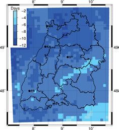
Meteorol. Z. (Contrib. Atm. Sci.)                        J.W. Schipper et al.: Tailored Climate Parameters                             49
28, 2019

                                    (a)                          (b)                                (c)

                                    (d)                          (e)                                 (f)
Figure 5: Consecutive days with weather conditions for salting (salting days) per year. (a,b,c) Observations (1971–2000). (d,e,f) Mean
expected changes from model simulations for 2021–2050 compared to 1971–2000. (a,d) Single-day cluster. (b,e) Two-to-five-days cluster.
(c,f) Six-days-and-more cluster. Black lines correspond to the Baden-Wuerttemberg regions. Hatched areas correspond to non-significant
change.

days per year (green in Figure 6a). However, adaption
will be needed as soon as the amount of salting days
decreases by 10 % or more in this region. Hence, a
change in color-coding from green to yellow was carried
out for each grid cell within the Stuttgart region for
which more than six simulations (which is more than
50 % of the maximum available simulation runs) expect
a decrease in days of 10 % or more for the near future
compared to the reference period. Except for a small
area in the southeast, this is the case for almost the entire
region (Figure 6b).
                                                                                      (a)                              (b)
                                                                       Figure 6: Results of the sensitivity assessment for the number of
3.2 Warm and dry summers                                               days with favorable weather conditions for salting, based on the
                                                                       experts’ experience in single administrative regions. As not for all
A warm and dry summer is defined as a summer (June,                    regions experts could be contacted or the tailored climate parameter
July, and August) that is at least 1 K, which is numeri-               was applicable, not all regions are colored. (a) Reference period
cally the same as 1 °C, higher than in, and the precipita-             (1971–2000). (b) Near future (2021–2050).
tion sum is less than 80 % of an average summer in the
reference period 1971–2000 (equation 3.2).
                                                                       year and the average summer temperature during the pe-
  warm and dry summer =                                                riod 1971–2000, respectively. Accordingly, the variables
         ⎧                                                             PJJA and PJJA,1971-2000 denote the precipitation sums.
         ⎪
         ⎪
         ⎪0
         ⎪
         ⎨                                                                 In most of the study region, one or two warm
         ⎪
         ⎪1, T JJA ≥ T JJA,1971–2000 + 1 [K] and           (3.2)       and dry summers occurred during the reference period
         ⎪
         ⎪
         ⎩    PJJA < PJJA,1971–2000 · 0.8                              1971–2000 (Figure 7a). In a few regions in the cen-
                                                                       ter and at the Southeast of the study region no warm
   In equation 3.2, the variables T JJA and T JJA,1971–2000            and dry summer was observed, according to the defini-
denote the average summer temperature for a specific                   tion in equation 3.2. Scattered in the West and North,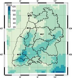
50                           J.W. Schipper et al.: Tailored Climate Parameters                           Meteorol. Z. (Contrib. Atm. Sci.)
                                                                                                                                 28, 2019

               (a)                             (b)
Figure 7: Number of warm and dry summers (June, July, August).
(a) Observations (1971–2000). (b) Mean expected changes from          Figure 8: Inter-annual variability (spatial average) of the number
model simulations for 2021–2050 compared to 1971–2000. The            of warm and dry summers in each model simulation (Table 2) for
color bar shows the sum of summers over 30 years (left) and the       the reference period and the observations (1971–2000, left panel)
corresponding annual mean value (right). Latter values are in line    and the near future (2021–2050, right panel). A cross denotes one
with the numbers in Figure 8.                                         year, a white circle the average value over the corresponding period.
                                                                      The black lines denote the average value over all models and all
                                                                      years in the corresponding period. A star (*) at a model name at the
some areas show three to four warm and dry summers in                 right panel (near future) denotes a significant change compared to
that period. For the reference period, the spatial and an-            the reference period for that particular simulation run.
nual mean over the entire study region is about 1.7 sum-
mers for the observations (corresponding to a mean of
0.05 summers per year) and about 2.6 summers for the                  period (seven crosses about 0.8 in Figure 8), whereas for
ensemble mean (corresponding to a mean of 0.09 sum-                   the near future, 20 such warm and dry summers are sim-
mers per year).                                                       ulated.
                                                                           Although the definition of a warm and dry summer
    The ensemble mean of the climate model simula-
                                                                      was the same, the sensitivity of such a summer was in-
tions for the near future shows a statistically significant
                                                                      terpreted differently in different fields of action. Experts
increase in the number of warm and dry summers for
                                                                      in the field of forestry stated the necessity for medium
the entire study region (no hatched areas in Figure 7b).
                                                                      adaptation measures in the administrative region hold-
Depending on the region, the number of warm and dry
                                                                      ing the city of Karlsruhe in the current climate (yellow in
summers increases between two and seven, with an av-
                                                                      Figure 9a). It was assessed that an increase in warm and
erage of 4.3 summers (corresponding to a mean of about
                                                                      dry summers of more than 10 % would require intensi-
0.14 summers per year). For both the observations and
                                                                      fied climate change adaptation. According to the model
the future changes, no dependency on elevation height is
                                                                      simulation results, this relative increase occurs in the en-
found.
                                                                      tire Karlsruhe region in at least 50 % (i.e. six) of the sim-
    As warm and dry summers do not occur every year,                  ulation runs for the near future (red in Figure 9b).
and are actually rather seldom (many crosses overlap at                    Experts from the administrative regions with Karls-
zero in Figure 8), the number of summers is not nor-                  ruhe and Freiburg in the field of pomiculture indicated a
mally distributed and, therefore, does not allow to cal-              different sensitivity to climate change adaptation than in
culate a standard deviation. As for each year, a value                the forest sector. In the climate of the reference period,
of 1 means that the entire study region had a warm and                it is already confronted with medium adaptation (yellow
dry summer, the value 0.05 for the observations means                 in Figure 9c). It is expected that an increase of 30 % and
that on average in 5 % of the study region a warm and                 more of warm and dry summers in the near future com-
dry summer occured each year. For the entire ensemble                 pared to the reference period will require strong climate
during the reference period, this is 9 % of the study re-             adaptation. According to simulation results, such an in-
gion. For the near future, the ensemble shows 0.23 sum-               crease is expected in at least 50 % (i.e. six) of the sim-
mers (corresponding to 23 % of the study region) on                   ulation runs for both entire regions (red in Figure 9d).
average. Single simulation runs initiated by CGCM3.1                  Actually, a more detailed look into the results gave that
and HadGEM2-ES even show numbers corresponding                        only three simulation runs resulted in an increase of less
to up to 38 and 37 %, respectively. Note that due to the              than 30 % for a few areas within these regions.
skewed distribution, the average number of the study re-
gion for each simulation run should be interpreted with               3.3 Years between warm and dry summers
care. Still, a clear increase in warm and dry summers in
the study region is found (Figure 8). Taking 80 % of the              Not only the warm and dry summers themselves, also
study region as an arbitrary limit to characterize an area-           the years in between such summers have been identified
wide impact, such a warm and dry summer is simulated                  by the experts to have a large impact on the well-being
seven times by the simulation ensemble for the reference              of the biosphere, especially trees. Therefore, the number
Meteorol. Z. (Contrib. Atm. Sci.) J.W. Schipper et al.: Tailored Climate Parameters 51
28, 2019
(a) (b) (a) (b)
Figure 10: Number of years between warm and dry summers
(June, July, August). (a) Observations (1971–2000). (b) Mean ex-
pected changes from model simulations for 2021–2050 compared to
1971–2000.
climate period of 30 years may not be sufficiently long
to draw conclusions about the actual period length be-
tween two warm and dry summers. We, however, notice
realistic regional differences in the study region, which
let us assume that the time frame may be appropriate for
(c) (d) a first look at the results. According to the observations,
Figure 9: Results of the sensitivity assessment for the number of the shortest average period lengths are found in the West
warm and dry summers with respect to forestry (a,b) and pomicul- and Northwest of the study region, whereas longer pe-
ture (c,d), based on the experts’ experience in single administrative riod lengths, associated with longer relaxation periods
regions. As not for all regions experts could be contacted or the tai- for the biosphere, are found in the East and Southeast of
lored climate parameter was applicable, not all regions are colored. the study region.
(a,c) Reference period (1971–2000). (b,d) Near future (2021–2050). The mean ensemble period length between warm
and dry summers decreases between two and twelve
years for the study region in 2021–2050 compared to
of years between warm and dry summers was calculated 1971–2000 (Figure 10b). In contrast to the absolute val-
analogously to the summers themselves (equation 3.3). ues in the observations, there is hardly any regional dif-
ferentiation in the decrease. This means that in the re-
year between warm and dry summers = gions, where short period lengths between warm and dry
⎧
⎪
⎪
⎪0 summers were already observed in the reference period,
⎪
⎨ the period length may go below a critical boundary.
⎪
⎪1, T JJA < T JJA,1971-=2000 + 1 [K] and (3.3)
⎪
⎪
⎩ The experts in the field of urban and regional plan-
PJJA ≥ PJJA,1971-2000 · 0.8
ning stated that currently the situation concerning the
Note that equation 3.3 is the exact opposite of equa- years between warm and dry summers requires medium
tion 3.2 and describes the number of summers, which are adaptation (yellow in Figure 11a). This statement was
not warm and dry. However, in contrast to the number of valid for the entire state of Baden-Wuerttemberg, except
warm and dry summers, the results of equation 3.3 for for the higher elevated regions, for which no information
the years in between are checked on consecutive years, could be given by our experts.
as not the number alone, but rather the gap in between For the near future, the experts stated that the yellow
two warm and dry summers is decisive for the biosphere. areas change to red as soon as there are less than five
If no warm and dry summer occurs during a 30 year years between two warm and dry summers, which is the
period, this equals to a gap of (at least) 30 years be- case for at least half of the simulation runs in all these
tween two warm and dry summers, assuming there could areas (red in Figure 11b). In fact, it was found that just
be one just before and after the considered period. One four out of twelve simulations runs did not fall below
warm and dry summer divides the 30 years period into this criteria and remained yellow at a few grid cells in
two gap-periods of 14.5 years on average, while the the South of Baden-Wuerttemberg (not shown).
number of four warm and dry summers on average oc-
curs after sequences of 5.2 years. Corresponding to zero 3.4 Hiking days
to four warm and dry summers in Figure 7a, the average
observed number of years in between are, therefore, ei- In this context, we define hiking as going for a hike
ther 30, 14.5, 9.33, 6.75, or 5.2 (Figure 10a). Actually, or a stroll with a duration of up to several hours. They
the maximum length may be even longer and the used are usually planned on short term or even spontaneously52 J.W. Schipper et al.: Tailored Climate Parameters Meteorol. Z. (Contrib. Atm. Sci.)
28, 2019
(a) (b) (a) (b)
Figure 11: Results of the sensitivity assessment for the number of Figure 12: Number of hiking days per year. (a) Observations
years between warm and dry summers with respect to urban and (1971–2000). (b) Mean expected changes from model simulations
regional planning, based on the experts’ experience in single ad- for 2021–2050 compared to 1971–2000.
ministrative regions. As not for all regions experts could be con-
tacted or the tailored climate parameter was applicable, not all re-
gions are colored. (a) Reference period (1971–2000). (b) Near future
precipitation criterion increases the number of days by
(2021–2050).
about 40 days on average, keeping the regional differen-
tiation roughly the same (not shown).
and, therefore, dependent on the prevailing weather con- The changes in number of hiking days in the near fu-
ditions. The tailored climate parameter hiking days may ture compared to the reference period differ throughout
not be of great relevance to the tourism industry as a the study region (Figure 12b). An increase in the number
whole, but it does, however, show the range of possible of hiking days is expected for the higher elevated areas,
applications of tailored climate parameters from climate because of an increase in the maximum temperatures in
model simulations. the near future. Whereas the upper boundary of 25 °C is
According to our experts from the tourism industry, not yet reached in these regions, temperatures are more
the maximum temperature at which it is still comfortable often above the lower boundary in winter. On the con-
to hike is 25 °C for most people. Above this temperature, trary, a decrease in hiking days is expected for the lower
most people search for alternative activities. The lowest elevated areas, like the Rhine Valley. Although the lower
temperature at which people start hiking is very depen- boundary is reached more often in those regions in the
dent on the time of the year, meaning that during winter near future, the upper boundary of 25 °C is more often
time, people go hiking at much lower temperatures, than exceeded, resulting in an overall decrease in the number
during summer time. To account for this behavior, we of hiking days. As both mechanisms of increasing and
chose a dynamical minimum daily maximum tempera- decreasing numbers compensate each other between the
ture (T day,max ). Also, too much precipitation makes the higher and lower elevated areas, the changes are very
people stay at home. All these criteria result in the defi- small in between and, therefore, to a large extent statis-
nition of a hiking day (equation 3.4). tically not significant (hatched areas).
The observed spatial averaged number of hiking days
hiking day = is about 224.6 days per year (Figure 13). The simula-
⎧ tion runs give a similar number of 225.4 days during
⎪
⎪
⎪0
⎪
⎨ the same time period. The average values for the sin-
⎪
⎪1, T day,max,month < T day,max < 25 [°C] and (3.4) gle simulation runs vary between 222.3 (boundary data
⎪
⎪
⎩ Pday,sum ≤ 5 [mm] from HadGEM2-ES) and 226.5 (boundary data from
ECHAM6) days. Also, the difference of standard devi-
The variable T day,max,month is dependent on the month ation between the observational data set (13.7 days) is
of the year and defined as follows: almost similar to the simulation runs for the reference
period (15.1 days). The expected slight increase of hik-
month T day,max,month ing days in the future from 225 to 227 days is very small
December, January, February 0 °C and statistically not significant. Only one single simula-
March, November 5 °C tion run (boundary data from ECHAM5-r2, which ex-
April, May, September, October 10 °C pects an increase from 223 to 232 days) does expect a
June, July, August 15 °C statistically significant change. The standard deviation
in the future stays the same, at 15.1 days. It should be
A dependency on elevation is observed for the num- noted that the differences between single years can be
ber of hiking days, with at higher elevations less hik- up to almost 100 days, taking into account all simula-
ing days, about 120–140 days, than at lower elevations, tion runs, and up to about 80 days for single simula-
about 240–280 days (Figure 12a). This is predominantly tion runs. Although, the regional differences already de-
due to the temperature criterion, because skipping the scribed at Figure 12 are expected to slightly decrease inYou can also read